High-resolution X-ray spectroscopy of the evolving shock in the 2006 outburst of RS Ophiuchi

Abstract

The evolution of the 2006 outburst of the recurrent nova RS Ophiuchi was followed with 12 X-ray grating observations with Chandra and XMM-Newton. We present detailed spectral analyses using two independent approaches. From the best dataset, taken on day 13.8 after outburst, we reconstruct the temperature distribution and derive elemental abundances. We find evidence for at least two distinct temperature components on day 13.8 and a reduction of temperature with time. The X-ray flux decreases as a power-law, and the power-law index changes from $-5/3$ to $-8/3$ around day 70 after outburst. This can be explained by different decay mechanisms for the hot and cool components. The decay of the hot component and the decrease in temperature are consistent with radiative cooling, while the decay of the cool component can be explained by the expansion of the ejecta. We find overabundances of N and of $\alpha$ elements, which could either represent the composition of the secondary that provides the accreted material or that of the ejecta. The N overabundance indicates CNO-cycled material. From comparisons to abundances for the secondary taken from the literature, we conclude that 20-40% of the observed nitrogen could originate from the outburst. The overabundance of the $\alpha$ elements is not typical for stars of the spectral type of the secondary in the RS Oph system, and white dwarf material might have been mixed into the ejecta. However, no direct measurements of the $\alpha$ elements in the secondary are available, and the continuous accretion may have changed the observable surface composition.

1. Introduction

Nova explosions occur in binary systems containing a white dwarf (WD) that accretes hydrogen-rich material from its companion. When $10^{-6}-10^{-4}$ M_⊙ have been accreted (depending on the WD mass), ignition conditions for explosive nuclear burning are reached and a thermonuclear runaway (TNR) occurs (Starrfield et al., 2008). Material dredged up from below the WD surface is mixed with the accreted material and violently ejected. While nuclear burning continues, the WD is surrounded by a pseudo atmosphere, and the peak of the spectral energy distribution (SED) shifts from the optical to soft X-rays as the radius of the pseudo photosphere shrinks (Gallagher & Starrfield, 1978). Observations of novae in soft X-rays therefore generally yield no detections until the photosphere recedes to the regions within the outflow that are hot enough to produce X-rays. For some novae this has been observed, and the X-ray spectra during this phase resemble the class of Super Soft X-ray Binary Sources (SSS, Kahabka & van den Heuvel, 1997). This phase is therefore called the SSS phase.

Observational evidence (from optical observations) and theoretical calculations indicate two abundance classes of novae, those with overabundance of carbon and oxygen (CO novae) and those with overabundance of oxygen and neon (ONe novae; see, e.g., Andrea et al. 1994; Jose & Hernanz 1998). Since the pressure on the white dwarf surface is not high enough for the production of C, O, or Ne during the nova outburst, these abundance classes reflect the composition of the WD. This indicates that core material is dredged-up into the accreted material and the gases are mixed before being ejected into space (Starrfield et al., 1998; Gehrz et al., 1998). In addition to dredged-up WD material, the ashes of CNO burning during the outburst have frequently been observed (Andrea et al., 1994; Jose & Hernanz, 1998). The composition of the ejected material is thus highly non-solar.

RS Oph is a Recurrent Symbiotic Nova, which erupts about every 20 years. The latest outburst occurred on 2006 February 12.83 (= day 0; Hirosawa et al., 2006). The mass donor is a red giant (M2III), and the expanding ejecta interact with the pre-existing stellar wind setting up shock systems. The composition of the red giant was studied by Pavlenko et al. (2008), who found that the overall metallicity does not seem to be significantly different from solar ($[$Fe/H$]=0.0\,\pm\,$0.5), C is underabundant ($[$C$]=-0.4$), and N overabundant ($[$N$]=+0.9$). UV spectra taken with IUE during the 1985 outburst provided evidence that N was overabundant (Shore et al., 1996). Lines of C were observed, but no detailed abundance analyses were carried out by Shore et al. (1996). Contini et al. (1995) determined an N/C abundance ratio of 100 and N/H=10 from optical spectra taken on day 201. From their absolute abundance of N and Fe, an abundance ratio of N/Fe=15 relative to solar can be derived. Snijders (1987a) found N/O=1.1 and C/N=0.16, and they caution that the evolved secondary can already be C/N depleted. Contini et al. (1995) found significant underabundance of O/H and of Ne/H of $\sim 10$% solar but high abundance ratios of Mg/Fe=5.4 and Si/Fe=7.2.

During the first month after outburst, intense hard X-ray emission, that originated from the shock, was observed with Swift and the Rossi X-ray Timing Explorer (RXTE; Bode et al. 2006; Osborne et al. 2008; Sokoloski et al. 2006). Swift X-Ray Telescope (XRT) observations carried out between days 3–26 were analyzed by Bode et al. (2006) who applied single-temperature MEKAL models to the X-ray spectra. They determined temperatures and wind column densities, $N_{\rm W}=N_{\rm H}({\rm total})-N_{\rm H}({\rm interstellar})$. The interstellar value of $N_{\rm H}({\rm interstellar})=2.4\times 10^{21}$ cm^-2 has been determined from H i 21 cm measurements (Hjellming et al., 1986). This value is consistent with the visual extinction ($E(B-V)=0.73\,\pm\,0.1$) determined from IUE observations in 1985 (Snijders, 1987b). Bode et al. (2006) converted the temperatures found from the MEKAL models into derived shock velocities $v_{\rm s}$, assuming that the X-rays were produced in the blast wave driven into the circumstellar material following the outburst. Before day $\sim 6$ after outburst they found a power-law decay $t^{-\alpha}$ with an approximate index $\alpha=0.6,\ 0.5$, and $1.5$ for $v_{\rm s}$, $N_{\rm W}$, and the flux (unabsorbed, i.e., corrected for interstellar absorption), respectively. These results compare well with model predictions of the RS Oph system presented by O’Brien et al. (1992 - see also Bode & Kahn 1985). According to these models, the evolution can be divided into three phases. The first phase (I), where the ejecta are still important in supplying energy to the shocked stellar wind of the red giant, lasts only a few days. The second phase (II) commences when the blast wave is being driven into the stellar wind and is effectively adiabatic. This phase is expected to last until the shocked material is well cooled by radiation (phase III). The physics behind these phases of evolution, together with the density distribution in the wind, determine the evolution of temperature with the corresponding velocity of the shock, unabsorbed fluxes, and the absorbing column of the wind (Vaytet et al., 2007).

Sokoloski et al. (2006) analyzed X-ray data taken between days 3–21 with RXTE, and from thermal bremsstrahlung models found that the temperature decreased with time $t$ as $t^{-2/3}$. They concluded that the speed of the blast wave produced in the nova explosion decreased with $t^{-1/3}$. However, the RXTE data with their low sensitivity at low energies did not favor the measurement of the wind column density $N_{\rm W}$.

A Chandra High Energy Transmission Grating Spectrograph snapshot of the blast wave obtained at the end of day 13 and analyzed by Drake et al. (2008) shows asymmetric emission lines sculpted by differential absorption in the circumstellar medium and explosion ejecta. Drake et al. (2008) found the lines to be more sharply peaked than expected for a spherically-symmetric explosion and concluded that the blast wave was collimated in the direction perpendicular to the line of sight, as also suggested by contemporaneous radio interferometry (O’Brien et al., 2006).

The SSS phase was observed after day $\sim 30$ and ended before day $\sim 100$ after outburst (Osborne et al., 2008). Three high-resolution X-ray spectra were taken during this phase which are described by Ness et al. (2007). The SSS emission longward of $\sim 12$ Å ($E>1$ keV) outshines any emission produced by the shock at these wavelengths, however, all emission shortward of 12 Å originates exclusively from the shock (Ness et al., 2008, 2007). We note that Bode et al. (2008) show tentative evidence for emission between 6-12 Å that may reflect the evolution of the SSS. The SSS spectra analyzed by Ness et al. (2007) contain emission lines on top of the bright SSS continuum which, combined with blue-shifted absorption lines, were first attributed to P Cygni profiles (Ness et al., 2006), but may also originate from the shock Ness et al. (2007).

An analysis of all X-ray grating spectra was presented by Nelson et al. (2008). They discovered a soft X-ray flare in week 4 of the evolution in which a new system of low-energy emission lines appeared. With their identifications of the emission lines, they derived velocities of $8,000-10,000$ km s^-1 which is consistent with the escape velocity of the WD, and the new component may thus represent the outflow. From preliminary atmosphere models they also determined the abundance ratio of Carbon to Nitrogen of 0.001 solar. This is a factor 10 lower than C/N abundance measurements by Contini et al. (1995) and a factor 100 lower than Snijders (1987a). From He-like line flux ratios they confirm that the shock plasma is collisionally dominated. They measured line shifts and line widths and found that the magnitude of the velocity shift increases for lower ionization states and longer wavelengths. In addition, as the wavelength increased, so did the broadening of the lines. They discuss bow shocks as a possible origin for the line emission seen in RS Oph. From multi-temperature plasma modelling of the early X-ray spectra, Nelson et al. (2008) needed four temperature components. While they found reasonably good reproduction of the Chandra spectrum, the same model was in poor agreement with the simultaneous XMM-Newton spectrum. Their model underpredicts lines of O and N, and they concluded that these elements are overabundant, and that the lines originated in the ejecta.

The structure of this paper is as follows: In §2 we present 12 X-ray grating observations taken between days 13.8 and 239.2 after outburst, focusing only on the emission produced by the shock. We measure emission line fluxes and line ratios in §3, and in §4 we present supporting models. We compute multi-temperature spectral models with the fitting program xspec (§4.2) and reconstruct a continuous temperature distribution based on a few selected emission lines (§4.3), yielding the elemental abundances. In §4.4 we compare the results of these two model approaches. We dedicate a separate section (§4.5) to the discussion of systematic uncertainties, as all given error estimates are only statistical uncertainties. In §5 we discuss our results and summarize our conclusions in §6.

2. Observations

Figure 1.— 11 X-ray grating spectra extracted from 12 Chandra and XMM-Newton observations taken on the dates and with the instruments given in the legends. Plotted are the raw spectra in counts per bin per individual exposure time (see Table 1). Bin sizes are 0.005 Å, 0.0025 Å, and 0.01 Å for MEG, HEG, and RGS1, RGS2, and LETG, respectively. Four Chandra spectra taken between days 204 and 208 after outburst are combined. RGS1 and RGS2 spectra are combined.

In this paper we analyze five X-ray grating spectra taken with Chandra and five with XMM-Newton. We use the High- and Low Energy Transmission Grating spectrometers (HETG and LETG, respectively) aboard Chandra and the Reflection Grating Spectrometers (RGS1 and RGS2) aboard XMM-Newton to obtain data between 1 Å and 40 Å. In Table 1 we list the start- and stop times, the corresponding days after outburst, the mission and instrumental setup, ObsIDs, and net exposure times for each observation. We have extracted the spectra in the same way as described by Ness et al. (2007) using the standard tools provided by the mission-specific software packages SAS (Science Analsis Software, version 7.0) and CIAO (Chandra Interactive Analysis of Observations, version 3.3.0.1). While pile up in the zero-th order of the Chandra HETGS observation may lead to problems in centroiding the extraction regions for the dispersed spectra (Nelson et al., 2008), we are confident that the standard centroiding is accurate enough. For example, the wavelengths of strong lines from the two opposite dispersion orders agree well with each other.

We have also extracted spectra from the XMM-Newton European Photon Imaging Camera (EPIC), concentrating on the observations recorded with the Metal Oxide Semi-conductor chips (MOS1). We have used standard SAS routines for the extraction of spectra and have corrected for pile up using annular extraction regions that avoid extracting photons from the innermost regions of the point spread function (PSF) following the instructions provided by the SAS software. We only need the MOS1 data for ObsID 0410180201 (26.1 days after outburst) in §4.2, for which an inner radius of 300 pix ($15\arcsec$) has to be excluded to avoid significant pile up.

Table 1Grating observations of RS Oph

Date	Daya	Mission	Grating	ObsID	exp. time
start–stop			/detector		(net; ks)
Febr. 26, 15:20	13.81	Chandra	HETG	7280	9.9
–Febr. 26, 18:46	13.88		/ACIS
Febr. 26, 17:09	13.88	XMM	RGS1  0410180101		23.8
–Febr. 26, 23:48	14.2		RGS2		23.8
March 10, 23:04	26.1	XMM	RGS1  0410180201		11.7
–March 11, 02:21	26.3		RGS2		11.7
March 24, 12:25	39.7	Chandra	LETG	7296	10.0
–March 24, 15:38	39.8		/HRC
April 07, 21:05	54.0	XMM	RGS1  0410180301		9.8
–April 08, 02:20	54.3		RGS2		18.6
April 20, 17:24	66.9	Chandra	LETG	7297	6.5
–April 20, 20:28	67.0		/HRC
June 04, 12:06	111.7	Chandra	LETG	7298	19.9
–June 04, 18:08	111.9		/HRC
Sept. 06, 01:59	205.3	XMM	RGS1  0410180401		30.2
–Sept. 06, 17:30	205.9		RGS2		30.2
Sept. 04, 10:43	203.6	Chandra	LETG	7390	39.6
–Sept. 04, 22:26	204.1		/HRC
Sept. 07, 02:37	206.3	Chandra	LETG	7389	39.8
–Sept. 07, 14:29	206.8		/HRC
Sept. 08, 17:58	207.9	Chandra	LETG	7403	17.9
–Sept. 08, 23:36	208.2		/HRC
Oct. 09, 23:38	239.2	XMM	RGS1  0410180501		48.7
–Oct. 10, 13:18	239.7		RGS2		48.7

^aafter outburst (2006, Feb. 12.83)

2.1. Description of spectra

An overview of all grating spectra is presented in Fig. 1 with the instrument and day after outburst indicated in the legends of each panel. All spectra taken on days 13.8 and 26.1 after outburst (top three panels) are characterized by a hard, broad continuum spectrum with additional strong emission lines (Ness et al., 2006; Drake et al., 2008). The count rate on day 26.1 is significantly lower than that on day 13.8, and the shape of the continuum is different. On day 26.1 a new component is observed longward of $\sim 20$ Å (Nelson et al., 2008) that could be associated with the SSS spectrum that was clearly detected three days later with Swift (Osborne et al., 2008). However, the spectral shape of this new component on day 26.1 is quite different from the spectra observed on days 39.7, 54.0, and 66.9 (next three panels). These spectra are dominated by the SSS spectrum (Ness et al., 2007) between 14 Å and 37 Å, while the emission from the shock dominates shortward of $\sim 15$ Å (Ness et al., 2008). After day $\sim 100$, the SSS spectrum has disappeared, and those spectra display emission lines with a weak continuum. The short-wavelength lines are only seen in the early spectra while those between 12 Å and 25 Å can be seen in all spectra, however, with different relative strengths.

Figure 2.— X-ray spectrum of RS Oph on day 13.8, in photon flux units, taken with Chandra/MEG shortward of 16.5 Å and with XMM-Newton/RGS longwards. We label H-like and He-like lines in italic font with the H-like lines in bold-face. Other lines are labeled with roman font. The high ionization stages indicate temperatures up to $10^{8}$ K while the additional presence of low-ionization stages show that the plasma is not isothermal.

In Fig. 2 we show the X-ray spectrum taken on day 13.8. For this plot we have converted the number of counts in each spectral bin to photon fluxes, simply dividing the number of counts by the effective areas extracted for each spectral bin from the instrument calibration. With grating spectra such a conversion is sufficiently accurate because of the precise placement of the recorded photons into the spectral grid. In contrast to low-resolution X-ray spectra taken with CCDs, the photon redistribution matrix of grating spectra is nearly diagonal. Below 16.5 Å we show the Chandra/MEG spectrum, and above this wavelength, where the MEG has extremely low sensitivity, the combined XMM-Newton/RGS spectra are shown. The strongest lines seen in the spectrum originate from H-like and He-like ions of S xvi and S xv (4.73 and 5.04 Å), Si xiv and Si xiii (6.18 and 6.65 Å), Mg xii and Mg xi (8.42 and 9.2 Å), Ne x and Ne ix (12.1 and 13.5 Å), O viii and O vii (18.97 and 21.6 Å), and N vii (24.78 Å). Also some of the 3p-1s lines are detected, e.g., Mg xii at 7.11 Å, Mg xi at 7.85 Å, and O viii at 16 Å. The H-like and He-like lines of elements with higher nuclear charge arise at shorter wavelengths, and strong lines at short wavelength indicate high temperatures. Several Fe lines are present, e.g., Fe xxv (1.85+1.86+1.87 Å) and Fe xxiv at 10.62 Å as well as low-ionization lines of Fe xvii at 15.01 Å and 12.26 Å. These lines cannot be formed in the same region of the plasma and it is thus not isothermal.

Figure 3.— XMM-Newton/RGS1 and RGS2 spectra (combined) taken on day 26.1 and converted to photon flux units. The strongest emission lines are labelled as explained in Fig. 2.

In Fig. 3 we show the combined XMM-Newton/RGS spectra taken on day 26.1, in the same units as in Fig. 2 for direct comparison. While on day 13.8 the strongest lines are formed at wavelengths shortward of 10 Å, the Ne x line at 12.1 Å is now the strongest line. This could mean that the temperature and/or the neutral hydrogen column density have decreased. The relative line strengths of H-like to He-like lines are significantly lower for all elements (see, e.g., Mg xii to Mg xi). This is clearly a temperature effect, and the plasma is cooling. Longwards of 25 Å a new component can be seen. The fact that only three days later the SSS spectrum was observed with Swift (Osborne et al., 2008) suggests that this emission represents the onset of the SSS phase (e.g., Bode et al., 2006; Nelson et al., 2008). However, while the SSS spectra observed on day 39.7 range from $\sim 15-30$ Å (Fig. 1), the RGS spectra shown in Fig. 3 show only excess emission longward of $\sim 20$ Å (see also Fig. 9). At 23.5 Å a deep absorption edge from O i has been found in the SSS spectra of RS Oph by Ness et al. (2007) (see also bottom panel of Fig. 9). The hard portion of an early faint SSS spectrum might be entirely absorbed by circumstellar neutral oxygen in the line of sight, while the shock-induced emission may originate from further outside, thus traversing through less absorbing material. Also, in the standard picture of nova evolution, the peak of the SED is expected to shift from long wavelengths to short wavelengths while the radius of the photosphere recedes to successively hotter layers, and the observed emission would be consistent with this picture. However, the spectrum has more characteristics of an emission line spectrum (see Fig. 3 and Nelson et al. 2008), but only the lines at 24.79 Å and 28.78+29.1+29.54 Å can be identified as N vii and as the N vi He-like triplet lines, respectively. In between the N vii and N vi lines no strong lines are listed in any of the atomic databases. The strongest emission line in this range is observed as a narrow line at 27.7 Å (FWHM 0.08 Å) with a line flux of $(2.7\,\pm\,0.4)\times 10^{-13}$ erg cm^-2 s^-1. The only possible identifications would be Ar xiv (27.64 Å and 27.46 Å) or Ca xiv (27.77 Å). Both appear rather unlikely identifications, as no Ar lines are detected in any of the other spectra, and for Ca xiv, stronger lines are expected at 24.03 Å, 24.09 Å, and 24.13 Å, but are not detected. A remarkable aspect is that the 27.7-Å line is so narrow while the N vii line shows an extremely broad profile (see §3.1). Another unidentified line is measured at 23.6 Å, but we experience the same difficulties in finding an identification. This could be residual continuum emission if the absorption feature at 23.5 Å is interpreted as interstellar O i. Nelson et al. (2008) suggested that some of these lines are blue-shifted N vi and C vi lines, but this requires extremely high velocities and is in contradiction to the non-detection of the C vi Ly$\alpha$ line and the low C abundance reported in the same paper. In any case, this component is likely not part of the shock systems, and the discussion of it is beyond the scope of this paper. While the O viii and O vii lines might be part of the shock, we treat the interpretation of these lines with care. We will also include the N vii line in our analyses as if it were formed in the shock, and any inconsistencies based on this line can be understood as supporting evidence that this component is unrelated to the shock emission. For more details of this component we also refer to Nelson et al. (2008).

Figure 4.— Same as Fig. 3 for the Chandra/LETG spectrum taken on day 39.7. Longward of $\sim 14.5$ Å the SSS spectrum dominates.

In Fig. 4 we show the photon flux spectrum taken with Chandra LETGS on day 39.7. The SSS spectrum dominates all emission longward of $\sim 14.5$ Å, and we only show the wavelength range relevant for this paper. The ratio of H-like to He-like lines is lower than in the earlier spectra, indicating that the temperature has continued to decrease. Since the lines are formed shortwards of the high-energy (Wien) tail of the SSS spectrum (14.5 Å$\approx 0.86$ keV), they are not affected by photoexcitations and originate exclusively from the shock.

Figure 5.— Same as Fig. 3 for the Chandra/LETG spectrum taken on day 111.7. The SSS spectrum has disappeared and emission lines longward of $\sim 14.5$ Å can be observed.

In Fig. 5 we show one of the spectra taken after the SSS had turned off. All emission lines are significantly weaker and the ratio of H-like and He-like lines is again lower than in the previous observation. All short-wavelength lines are extremely weak or are not detected.

Next we integrate the photon flux spectra over the range 7–11 Å (1.1–1.8 keV) in order to obtain X-ray fluxes. We do not correct for absorption, thus yielding fluxes at Earth. Since the fluxes are extracted from above 1 keV, the effects from absorption are small, and particularly the relative evolution of the absorbed and non-absorbed fluxes is the same. The wavelength range over which the fluxes are integrated is a compromise between collecting as much information as possible from the observations before day 39.7 and after day 66.9 while excluding as much as possible of the emission from the SSS on days 39.7, 54.0, and 66.9. The results are illustrated as a function of time in Fig. 6. For comparison we include rescaled Swift/XRT count rates (0.25-10 keV) taken after day 106. At this late stage of the evolution, the spectral shape hardly changes (see Table 5), yielding a direct correlation between X-ray flux and count rate. With the assumption of no spectral changes between days 106 and 250, we can also use the count rates integrated over the full Swift XRT band pass, as additional emission in the larger wavelength range also scales directly with the count rate. Since we are not interested in the absolute flux from the Swift observations, we chose a scaling factor of $3\times 10^{-12}$ erg cm^-2 s^-1 cps^-1 to yield the same values as the grating fluxes for days 111.7-239.2. The rescaled XRT count rate follows the same trend as the fluxes obtained from the grating spectra. We include two power-law curves, and the early evolution evolves more like $t^{-5/3}$, while the later evolution (after day 100) clearly follows a $t^{-8/3}$ trend. We observe the same behavior if we use a larger wavelength range and exclude the observations between days 39.7 and 66.9.

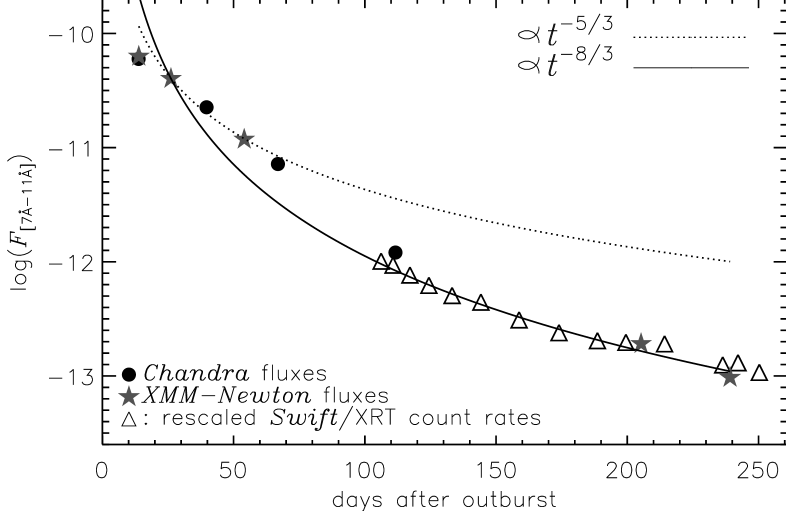
Figure 6.— X-ray fluxes measured at Earth (cgs units, integrated over 7–11 Å; 1.1–1.8 keV) as a function of time. The triangles mark Swift/XRT count rates (0.3-10 keV), rescaled by $3\times 10^{-12}$ [erg cm^-2 s^-1 cps^-1]. The statistical errors are smaller than the plot symbols. For systematic errors see §4.5.

3. Measurement of emission lines

3.1. Line shifts and profiles

In order to determine velocities from the emission lines we have measured wavelengths and line widths in excess of the instrumental line broadening function for a number of strong lines with well-identified rest wavelengths, $\lambda_{0}$. For the narrow wavelength range around the lines we have accounted for continuum emission by defining a constant local offset on top of the instrumental background that can be treated as an ’uninteresting’ free parameter. For each line $j$ we have used a normalized Gaussian profile with wavelength $\lambda_{j}$ and line width $\sigma_{j}$ and folded this profile through the instrumental response using the IDL tool scrmf provided by the PINTofAle package (Kashyap & Drake, 2000) before comparing with the measured count spectra. We have determined the statistical measurement uncertainties for $\lambda_{j}$ and $\sigma_{j}$ from the $2\times 2$ Hesse matrix as defined in Eq. 2 of the appendix section, which is based on an approach proposed by Strong (1985). Systematic uncertainties are difficult to assess and are not included in our error estimates (for details see §4.5). Those can arise from fluctuations in the underlying continuum and line blends. While the former has a stronger effect on weak lines, the latter can affect any line. For this reason we chose lines for which no strong nearby lines are known to arise. We have iterated $\lambda_{j}$ and $\sigma_{j}$, and in each iteration step we have adjusted the normalization utilizing the fixed point iteration scheme described by Ness & Wichmann (2002). The normalization factor can be converted to line fluxes (see §3.2).

The results are listed in Table 2. The line shifts $\lambda_{j}-\lambda_{0}$ and Gaussian line widths $\sigma_{j}$ (both measured in mÅ$=10^{-3}$Å) are converted to corresponding Doppler velocities using the rest wavelengths $\lambda_{0}$ listed in the first column. The measurement uncertainties of line shifts and widths are correlated uncertainties, and account for the uncertainties in the respective other values. The Ne x line at 10.23 Å is relatively weak in all observations, and the results from this line may be less certain due to additional systematic uncertainties from fluctuations in the underlying continuum. The Fe xvii line could be blended with the weak O viii 1s-4p ($\lambda_{0}=15.18$ Å) line, and the accuracy of the results from this line might suffer from line blending. All lines measured from observations taken after day 26.1 are weaker, and the uncertainties on the results from these observations have to be increased by at least 20% due to fluctuations in the continuum.

Figure 7.— Measurement of line shifts (left panels) and line widths (right panels) for the Chandra HETGS (bullets) and XMM-Newton (open boxes) observations taken on day 13.8 with the conversion to velocities, if interpreted as Doppler velocities (bottom panels). The error bars are statistical uncertainties only. For systematic errors see §4.5.

In Fig. 7 we illustrate the measured line shifts (top left) and widths (top right) and the corresponding velocities (respective bottom panels) for the observations taken on day 13.8. All lines are significantly blue-shifted, the short-wavelength lines by $200-800$ km s^-1 and the lines of O viii, O vii, and N vii at longer wavelengths by more than $1200$ km s^-1. Nelson et al. (2008) found similar values and concluded that there was a trend of increased velocities with wavelength and thus with formation temperature. However, with a different set of lines we come to a different conclusion. First, we have not used the unresolved He triplet lines of Mg xi and Si xiii to avoid additional systematic uncertainties from line blends (see §4.5). Then, we have included the Ne x and Fe xvii lines that lie in between the Mg lines and the O viii line. Although we caution that these lines may suffer from additional systematic uncertainties, there seems to be more of an abrupt change rather than a systematic trend with these additional lines included. Interestingly, the lines with larger blue shifts originate only from oxygen and nitrogen. Drake et al. (2008) investigated the possibility that the line profiles are dominated by complex absorption patterns in their red wings, leading to apparent blue shifts. In that case the column density in the respective line is a stronger driver for line shifts than the temperature, and oxygen and nitrogen might exhibit deeper column densities than other elements, possibly owing to higher elemental abundances.

The line widths are all about $800-1000$ km s^-1, with the exceptions of Ne x (10.23 Å) and Fe xvii (15.01 Å and 16.78 Å) which are narrower (bottom right panel of Fig. 7). Since fluctuations in the continuum and line blending cannot lead to narrower lines, it is not clear to us why these particular lines are narrower, but we cannot confirm a trend with long-wavelength lines being broader as reported by Nelson et al. (2008). Nelson et al. seem not to have accounted for the instrumental line broadening when computing line widths, but the instrumental line broadening is only $\sim 0.01$ Å for the MEG and $\sim 0.03$ Å in the RGS. The instrumental line profile is roughly Gaussian, and since the convolution of two Gaussians is again a Gaussian, the resulting line width is dominated by the broader line, and in the case of most lines, the instrumental line broadening can be neglected.

After day 13.8, all line shifts except those for the O viii and N vii lines fluctuate around the same value of $\sim 500-800$ km s^-1 (see Table 2). The O and N lines that show extreme blue-shifts on day 13.8 (Fig. 7) have values consistent with other lines in all later observations. If these lines are shaped by absorption in their red wings as proposed by Drake et al. (2008), then the column densities have decreased from day 13.8 to day 261. The N vii line on day 26.1 shows an extreme value (also in line width, see bottom panel of Fig. 7), and belongs to the new component discovered by Nelson et al. (2008); however, the velocity measured from the shift of this line does not agree with their value of 8,000-10,000 km s^-1 derived from the lines between 25–30 Å. While we mark these lines as unidentified in Fig. 3, Nelson et al. (2008) discuss possible identifications as highly blue-shifted N vi and C vi lines.

The line widths slowly decrease with time. The N vii line at 24.78 Å is extremely broad on day 26.1. At this time of the evolution, this line is part of the new component reported by Nelson et al. (2008) with a set of unidentified lines. There is thus a reasonable chance that this line is a blend, making this anomalous velocity questionable. Since shock velocities derived from the temperatures from the spectral models discussed in §4.2 represent the evolution of the expansion velocity, they can be compared with these values. The shock velocities derived from the hottest model component are given in the last row of Table 2. We discuss the implication of the comparison in §4.2.

Table 2Evolution of line shifts and line widths.

$\lambda_{0}^{a}$(Å)	day 13.81	day 13.88	day 26.1	day 39.7	day 54.0	day 66.9	day 111.7
ID	HETG	RGS	RGS	LETG	RGS	LETGS	LETGS
4.73  $\Delta\lambda$ (mÅ)	$-8.3\,\pm\,1.6$	–	–	–	–	–	–
S xvi $\sigma$ (mÅ)	$12.7\,\pm\,1.7$	–	–	–	–	–	–
$v_{\rm shift}$ (km s-1)	$-526\,\pm\,103$	–	–	–	–	–	–
$v_{\rm width}$ (km s-1)	$806\,\pm\,111$	–	–	–	–	–	–
6.18  $\Delta\lambda$ (mÅ)	$-8.1\,\pm\,0.6$	$-4.8\,\pm\,5.7$	–	$-16.1\,\pm\,5.2$	–	–	–
Si xiv $\sigma$ (mÅ)	$16.3\,\pm\,0.6$	$<12.1$	–	$17.7\,\pm\,8.9$	–	–	–
$v_{\rm shift}$ (km s-1)	$-395\,\pm\,29$	$-233\,\pm\,275$	–	$-781\,\pm\,253$	–	–	–
$v_{\rm width}$ (km s-1)	$790\,\pm\,27$	$<586.2$	–	$861\,\pm\,433$	–	–	–
8.42  $\Delta\lambda$ (mÅ)	$-21.3\,\pm\,0.7$	$-22.4\,\pm\,1.5$	$-6.5\,\pm\,2.9$	$-25.9\,\pm\,3.0$	$-17.5\,\pm\,0.7$	$-16.7\,\pm\,8.8$	$2.3\,\pm\,18.0$
Mg xii $\sigma$ (mÅ)	$26.5\,\pm\,0.6$	$23.0\,\pm\,3.0$	$20.3\,\pm\,5.3$	$24.0\,\pm\,5.3$	$<17.1$	$<11.0$	$<27.7$
$v_{\rm shift}$ (km s-1)	$-759\,\pm\,24$	$-796\,\pm\,54$	$-230\,\pm\,102$	$-924\,\pm\,107$	$-623\,\pm\,25$	$-593\,\pm\,313$	$82\,\pm\,640$
$v_{\rm width}$ (km s-1)	$945\,\pm\,21$	$818\,\pm\,108$	$724\,\pm\,189$	$853\,\pm\,187$	$<607.8$	$<390.6$	$<985.1$
10.23  $\Delta\lambda$ (mÅ)	$-14.2\,\pm\,2.3$	–	–	–	$-2.2\,\pm\,8.4$	$-17.9\,\pm\,10.7$	$-1.3\,\pm\,16.4$
Ne x $\sigma$ (mÅ)	$14.5\,\pm\,2.6$	–	–	–	$<11.3$	$<25.7$	$<12.1$
$v_{\rm shift}$ (km s-1)	$-416\,\pm\,69$	–	–	–	$-64\,\pm\,246$	$-525\,\pm\,314$	$-38\,\pm\,482$
$v_{\rm width}$ (km s-1)	$425\,\pm\,75$	–	–	–	$<331.7$	$<753.7$	$<355.1$
12.13  $\Delta\lambda$ (mÅ)	$-29.1\,\pm\,1.9$	$-17.6\,\pm\,2.4$	$-6.1\,\pm\,2.5$	$-19.3\,\pm\,2.6$	$-3.5\,\pm\,3.3$	–	$-6.8\,\pm\,5.6$
Ne x $\sigma$ (mÅ)	$34.0\,\pm\,1.6$	$38.0\,\pm\,3.7$	$24.3\,\pm\,4.4$	$27.3\,\pm\,4.0$	$29.7\,\pm\,5.6$	–	$<19.0$
$v_{\rm shift}$ (km s-1)	$-719\,\pm\,47$	$-435\,\pm\,60$	$-151\,\pm\,62$	$-477\,\pm\,65$	$-87\,\pm\,81$	–	$-168\,\pm\,139$
$v_{\rm width}$ (km s-1)	$841\,\pm\,39$	$939\,\pm\,91$	$601\,\pm\,110$	$675\,\pm\,99$	$733\,\pm\,137$	–	$<469.3$
15.01  $\Delta\lambda$ (mÅ)	$-14.8\,\pm\,3.3$	$12.7\,\pm\,4.8$	$4.1\,\pm\,3.2$	–	–	–	$18.3\,\pm\,4.5$
Fe xvii $\sigma$ (mÅ)	$19.7\,\pm\,4.4$	$65.5\,\pm\,5.8$	$30.5\,\pm\,4.4$	–	–	–	$28.3\,\pm\,3.0$
$v_{\rm shift}$ (km s-1)	$-296\,\pm\,65$	$254\,\pm\,96$	$82\,\pm\,64$	–	–	–	$365\,\pm\,91$
$v_{\rm width}$ (km s-1)	$394\,\pm\,89$	$1308\,\pm\,115$	$609\,\pm\,89$	–	–	–	$565\,\pm\,60$
16.78  $\Delta\lambda$ (mÅ)	$-19.8\,\pm\,7.3$	$-29.6\,\pm\,6.5$	–	–	–	–	$-38.9\,\pm\,8.5$
Fe xvii $\sigma$ (mÅ)	$15.1\,\pm\,7.3$	$13.3\,\pm\,11.2$	–	–	–	–	$<14.1$
$v_{\rm shift}$ (km s-1)	$-354\,\pm\,131$	$-529\,\pm\,116$	–	–	–	–	$-695\,\pm\,151$
$v_{\rm width}$ (km s-1)	$270\,\pm\,130$	$238\,\pm\,201$	–	–	–	–	$<252.6$
18.97  $\Delta\lambda$ (mÅ)	$-79.7\,\pm\,9.6$	$-82.6\,\pm\,2.8$	$-38.1\,\pm\,5.2$	–	–	–	$-26.3\,\pm\,3.0$
O viii $\sigma$ (mÅ)	$57.2\,\pm\,5.7$	$53.5\,\pm\,3.1$	$68.3\,\pm\,3.0$	–	–	–	$<1.0$
$v_{\rm shift}$ (km s-1)	$-1260\,\pm\,151$	$-1305\,\pm\,44$	$-602\,\pm\,82$	–	–	–	$-416\,\pm\,47$
$v_{\rm width}$ (km s-1)	$904\,\pm\,91$	$845\,\pm\,50$	$1080\,\pm\,48$	–	–	–	$<16.1$
24.78  $\Delta\lambda$ (mÅ)	–	$-106.9\,\pm\,6.3$	$30.0\,\pm\,7.7$	–	–	–	$-6.9\,\pm\,0.4$
N vii $\sigma$ (mÅ)	–	$82.2\,\pm\,5.9$	$170.3\,\pm\,1.5$	–	–	–	$<7.9$
$v_{\rm shift}$ (km s-1)	–	$-1293\,\pm\,76$	$363\,\pm\,93$	–	–	–	$-83\,\pm\,4$
$v_{\rm width}$ (km s-1)	–	$994\,\pm\,72$	$2060\,\pm\,18$	–	–	–	$<95.7$
$v_{\rm shock}(T_{1})$ (km s-1)b	$1899\,\pm\,22$		$1284\,\pm\,30$	$1269\,\pm\,44$	–	–	$792\,\pm\,37$
$v_{\rm shock}(T_{2})$ (km s-1)b	$792\,\pm\,8$		$792\,\pm\,8$	$714\,\pm\,7$	–	$747\,\pm\,60$	$548\,\pm\,61$

^arest wavelengths  ^bFrom k$T_{1}$ and k$T_{2}$ in APEC models

3.2. Line fluxes

We have used our line fitting program Cora (Ness & Wichmann, 2002) to measure line counts which are then converted to line fluxes using the effective areas extracted from the instrument calibration. The Cora program applies the likelihood method described in the appendix and adds a model of line templates to the instrumental background. In order to measure the line fluxes on top of the continuum, we have added a constant source background to the instrumental background before fitting. The continuum is not expected to change significantly over the narrow wavelength range considered for line fitting.

In Table 3 we list the measured line fluxes for the strongest lines of Fe and the H-like and He-like lines of N, O, Ne, Mg, Si, and S, sorted by wavelength (for emission line fluxes measured on days 39.7, 66.9, and 54 we refer to Ness et al. 2007). The given uncertainties are the statistical uncertainties. Additional systematic uncertainties arise from the assumed level of the underlying continuum and line widths (see §4.5). The fluxes are not corrected for the effects of interstellar or circumstellar absorption. In the bottom part of Table 3 we list line ratios of H-like to He-like line fluxes, which are temperature and density indicators.

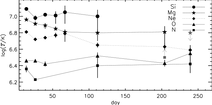
Figure 8.— Evolution of average temperatures derived from ratios of H-like and He-like lines for the elements given in the legend. The values are listed in Table 4. Error bars are statistical errors; systematic errors are small (see §4.5).

In the top part of Table 4 we list temperatures derived from the H-like to He-like line ratios of the same species (after correction for $N_{\rm H}$ as noted in Table 4) using theoretical predictions of the same ratios as a function of temperature extracted from an atomic database computed by the Astrophysical Plasma Emission Code (APEC, v1.3: Smith et al., 2001a, b). The temperatures are computed under the assumption of collisional equilibrium (see end of this section and §4.1 for more details) and are average values assuming that the plasma is isothermal over the temperature range over which the respective H-like and He-like lines are formed. Lines originating from high-Z elements probe hotter plasma. Since the lines involved in each ratio are from the same element, these ratios yield temperatures independently of the elemental abundances (see, e.g., Schmitt & Ness, 2004; Ness et al., 2005). A graphical representation is given in Fig. 8, and it can be seen that the Si ratios probe hotter plasma than the N ratios. Significantly different temperatures are derived, indicating that we are dealing with a wide range of temperatures in the early observations (before day $\sim 70$). The measurements for the later observations deliver consistent temperatures (at least within the large uncertainties), indicating that the plasma could be characterized by a single temperature by that time. The temperatures derived from the Mg lines indicate that the hotter plasma cools until day $\sim 70$ and remains constant after that time. A similar behavior can be concluded from the other values but it is not as clear. For example the temperatures derived from the Ne lines yield a slight increase, however, the temperature on day 26.1 may also be anomalously low, owing to line blends of the Ne ix lines (Ness et al., 2003a). We note that the N lines observed on day 26.1 show a peculiar behavior in the line shifts and -widths (see Table 2), and the derived temperature may thus not represent the same plasma as the values for the other times of evolution. For days 39.7-66.9 the cool component cannot be probed because the O and N lines are outshone by the SSS emission from the WD. The temperature derived from the O lines for day 39.7 is based on the fluxes measured by Ness et al. (2007) on top of the SSS continuum. These fluxes may be contaminated by photoexcitations, but the derived temperature agrees well with the temperatures derived for the other days.

In the bottom part of Table 4 we list densities derived from the He-like forbidden-to-intercombination (f/i) line ratios for the ions O vii and Ne ix. These values have been derived assuming collisional equilibrium according to the parameterization derived by Gabriel & Jordan (1969), neglecting UV radiation; see, e.g., Ness et al. (2004) for details. The method explores density-dependent excitations out of the upper level of the f line (1s2p ³S) into that of the i line (1s2p ³P). In the low-density limit, all ions in the 1s2p ³S state radiate to the ground (1s^2 1S), giving rise to the f line, while with increasing density, collisional excitations from the 1s^2 3S state into the 1s2p ³P state reduce the f line and increase the i line. However, the 1s2p ³P-1s2p ³S transition can also be induced by UV radiation, whose presence would mimic a high density if neglected (Blumenthal et al., 1972; Ness et al., 2001). Especially for the early spectra we must assume that significant UV contamination from the WD has to be accounted for. While the UV intensity can be estimated from IUE observations of the 1985 outburst (Shore et al., 1996), the distance between the X-ray emitting plasma and the UV source needs to be known in order to quantify the contaminating effects for the density diagnostics. Since UV radiation fields, if present, mimic high densities, we treat the values with great caution, but we can at least conclude that the density is not higher than any of the values listed in Table 4.

In the next section we present models for which the assumption of optically thin plasma is made. As a test of this assumption we measure the line flux ratio of the Ly$\beta$ (3p-1s) to Ly$\alpha$ (2p-1s) lines of the H-like ion Ne x (10.23 Å and 12.12 Å, respectively), which increases with increasing optical depth, but also depends on the electron temperature and the amount of photoelectric absorption in the line of sight. Theoretical predictions of the same ratio for an optically thin plasma in collisional equilibrium, from the atomic databases CHIANTI version 5.2 (Landi et al., 2006) and APEC, vary between 0.1 and 0.3 within the temperature range $10^{6}$ to $10^{8}$ K, while for day 13.8 we measure a ratio of $0.17\,\pm\,0.02$. This is well within the expected range. We also refer to the tests presented by Nelson et al. (2008) who measured the so-called G-ratio of the He-like triplets of S, Si, and Mg and concluded that the plasma is collisionally dominated.

Table 3Evolution of emission line fluxes.

		fluxb	fluxb	fluxb	fluxb	fluxb	fluxb	fluxb
Ion	$\lambda_{0}^{a}$(Å)	day 13.81	day 13.88	day 26.1	day 111.7	day 205.9	days 204–208e	day 239.2
Fe xxvi	1.78	$<144$	–	–	–	–	–	–
Fe xxvc	1.85	$1037\,\pm\,190$	–	–	–	–	–	–
S xvi	4.73	$219\,\pm\,22$	–	day 39.7: $<33.8$		–	–	–
S xvc	5.04	$624\,\pm\,84$	–	day 39.7: $78.1\,\pm\,67.7$		–	–	–
Si xiv	6.18	$349\,\pm\,13$	$260\,\pm\,32$	$138\,\pm\,29$	$2.7\,\pm\,1.8$	–	$<1.5$	–
Si xiiic	6.65	$620\,\pm\,32$	$795\,\pm\,112$	$560\,\pm\,124$	$10.3\,\pm\,5.6$	–	$<5.1$	–
Mg xii	8.42	$412\,\pm\,11$	$585\,\pm\,19$	$269\,\pm\,19$	$5.1\,\pm\,2.0$	$<0.3$	$1.3\,\pm\,0.7$	$<0.3$
Mg xic	9.20	$383\,\pm\,30$	$369\,\pm\,35$	$374\,\pm\,47$	$18.8\,\pm\,7.6$	$4.5\,\pm\,2.9$	$4.1\,\pm\,2.4$	$2.2\,\pm\,1.1$
Ne x	12.13	$273\,\pm\,20$	$309\,\pm\,9.2$	$309\,\pm\,12$	$21.6\,\pm\,3.0$	$3.0\,\pm\,0.7$	$3.2\,\pm\,0.7$	$2.0\,\pm\,0.5$
+Fe xvii	12.12	1.08 times the flux at 12.26 Å if $\log T<6.9$ otherwise negligible
Fe xvii	12.26	$52.8\,\pm\,6.8$	$52.5\,\pm\,6.6$	$82.8\,\pm\,9.3$	$3.2\,\pm\,1.8$	$<1.6$	$1.5\,\pm\,0.6$	$<0.75$
+Fe xxi	12.28	at $\log T>6.9$ only Fe xxi otherwise only Fe xvii
Ne ix	13.44	$71.8\,\pm\,8.9$	$99.8\,\pm\,5.3$	$148\,\pm\,9.4$	$19.6\,\pm\,2.8$	$3.7\,\pm\,0.8$	$3.4\,\pm\,0.7$	$3.1\,\pm\,0.5$
Ne ix (i)d	13.55	$19.8\,\pm\,6.8$	$38.2\,\pm\,4.5$	$60.3\,\pm\,8.4$	$3.4\,\pm\,1.8$	$1.2\,\pm\,0.6$	$1.0\,\pm\,0.6$	$0.7\,\pm\,0.4$
Ne ix (f)d	13.69	$33.9\,\pm\,6.8$	$53.3\,\pm\,4.1$	$82.3\,\pm\,7.4$	$10.1\,\pm\,2.1$	$3.3\,\pm\,0.7$	$2.8\,\pm\,0.6$	$2.4\,\pm\,0.5$
Fe xvii	14.21	$33.6\,\pm\,7.5$	$45.5\,\pm\,3.4$	$59.5\,\pm\,5.6$	$1.8\,\pm\,1.4$	$1.6\,\pm\,0.6$	$1.0\,\pm\,0.5$	–
Fe xvii	15.01	$67.3\,\pm\,8.1$	$69.5\,\pm\,3.6$	$156\,\pm\,7.7$	$14.3\,\pm\,2.1$	$3.4\,\pm\,0.7$	$2.7\,\pm\,0.5$	$2.7\,\pm\,0.5$
O viii	18.97	$84.2\,\pm\,19$	$92.5\,\pm\,3.1$	$186\,\pm\,13$	$33.5\,\pm\,2.8$	$7.7\,\pm\,1.4$	$5.3\,\pm\,0.6$	$5.2\,\pm\,0.5$
O vii	21.60	–	$14.8\,\pm\,1.9$	$29.5\,\pm\,3.1$	$6.8\,\pm\,1.8$	$2.4\,\pm\,0.5$	$2.1\,\pm\,0.6$	$0.9\,\pm\,0.3$
O vii (i)d	21.80	–	$<1.5$	$13.6\,\pm\,2.4$	$1.3\,\pm\,1.3$	$1.4\,\pm\,0.4$	$<0.5$	$0.6\,\pm\,0.3$
O vii (f)d	22.10	–	$6.4\,\pm\,1.3$	$33.4\,\pm\,3.2$	$5.4\,\pm\,1.7$	$2.0\,\pm\,0.5$	$0.8\,\pm\,0.6$	$1.0\,\pm\,0.3$
N vii	24.78	–	$43.0\,\pm\,1.8$	$259\,\pm\,12.8$	$15.7\,\pm\,2.3$	$6.6\,\pm\,0.7$	$3.9\,\pm\,0.6$	$4.0\,\pm\,0.5$
N vi	28.78	–	$2.3\,\pm\,0.6$	$35.4\,\pm\,3.5$	$1.8\,\pm\,1.1$	$<0.4$	$<1.5$	$0.4\,\pm\,0.2$
C vi	33.74	–	$<0.6$	$<0.5$	$<1.4$	$<0.3$	$<0.9$	$<0.1$
Temperature-sensitive line ratios
Fe xxvi/Fe xxv		$<0.2$	–	–	–	–	–	–
S xvi/S xv		$0.35\,\pm\,0.06$	–	day 39.7: $<3.25$		–	–	–
Si xiv/Si xiii		$0.56\,\pm\,0.04$	$0.33\,\pm\,0.06$	$0.25\,\pm\,0.08$	$0.26\,\pm\,0.23$	–	–	–
Mg xii/Mg xi		$1.08\,\pm\,0.09$	$1.59\,\pm\,0.16$	$0.72\,\pm\,0.10$	$0.27\,\pm\,0.15$	$<0.2$	$0.32\,\pm\,0.25$	$<0.3$
Ne ix/Ne x		$3.80\,\pm\,0.54$	$3.09\,\pm\,0.19$	$2.10\,\pm\,0.16$	$1.10\,\pm\,0.22$	$0.81\,\pm\,0.26$	$0.94\,\pm\,0.28$	$0.65\,\pm\,0.19$
O viii/O vii		–	$6.25\,\pm\,0.83$	$6.31\,\pm\,0.79$	$4.93\,\pm\,1.37$	$3.21\,\pm\,0.89$	$2.52\,\pm\,0.78$	$5.78\,\pm\,2.00$
N vii/N vi		–	$18.70\,\pm\,4.94$	$7.32\,\pm\,0.81$	$8.72\,\pm\,5.48$	$>14.8$	$>2.2$	$10.00\,\pm\,5.15$
Density-sensitive line ratios
Ne ix (f/i)		$1.7\,\pm\,0.7$	$1.4\,\pm\,0.2$	$1.4\,\pm\,0.2$	$3.0\,\pm\,1.7$	$2.8\,\pm\,1.5$	$2.8\,\pm\,1.8$	$3.4\,\pm\,2.1$
O vii (f/i)		–	$>4.3$	$2.5\,\pm\,0.5$	$>4.2$	$1.4\,\pm\,0.5$	$>4.0$	$1.7\,\pm\,1.0$

Uncertainties and upper limits are 68.3%. Additional systematic uncertainties are discussed in §4.5. $\bullet$ ^arest wavelengths $\bullet\ ^{b}10^{-14}$ erg cm^-2 s^-1 $\bullet\ ^{c}$sum of three lines $\bullet\ ^{d}$intersystem line $\bullet\ ^{e}$Sum of Chandra spectra taken between days 203.3 and 208.2 (see Table 1).

Table 4Temperatures and Densities derived from H-like to He-like line ratios

Ion	day 13.81	day 26.1	day 39.7	day 54	day 66.9	day 111.7	days 204–208a	day 239.2
$\log T$ in K, after correction of line ratios for $N_{\rm H}$ with values $5\times 10^{21}$ cm-2 for days 13.8 and 26.1 and $2.4\times 10^{21}$ cm-2 for the rest.
Fe	$<7.8$	–	–	–	–	–	–
S	$7.21^{+0.02}_{-0.20}$	–	$<7.61$	–	–	–	–
Si	$7.09\,\pm\,0.01$	$6.98\,\pm\,0.03$	$7.02\,\pm\,0.02$	$7.01^{+0.05}_{-0.1}$	$7.05^{+0.08}_{-0.14}$	$7.00^{+0.08}_{-0.19}$	–	–
Mg	$6.96\,\pm\,0.01$	$6.91\,\pm\,0.02$	$6.87\,\pm\,0.02$	$6.85\,\pm\,0.02$	$6.81\,\pm\,0.03$	$6.80^{+0.04}_{-0.1}$	$6.81^{+0.07}_{-0.16}$	$<6.8$
Ne	$6.81\,\pm\,0.02$	$6.72\,\pm\,0.01$	$6.74\,\pm\,0.02$	$6.77\,\pm\,0.03$	$6.79^{+0.05}_{-0.1}$	$6.65\,\pm\,0.03$	$6.63\,\pm\,0.04$	$6.59\,\pm\,0.03$
O	$6.46\,\pm\,0.02$	$6.46\,\pm\,0.02$	$6.42\,\pm\,0.03$	–	–	$6.52\,\pm\,0.04$	$6.43\,\pm\,0.04$	$6.55^{+0.05}_{-0.1}$
N	$6.36\,\pm\,0.04$	$6.23\,\pm\,0.01$	–	–	–	$6.40^{+0.08}_{-0.15}$	$>6.5$	$6.42\,\pm\,0.11$
Densities, $\log n_{e}$ in cm-3, from He-like triplet ratios assuming no UV illumination (see text §3.2)
O vii	$<8$	$10.3^{+0.7}_{-0.2}$	–	–	–	$<8$	$10.7^{+0.2}_{-0.8}$	$10.6^{+0.2}_{-0.8}$
Ne ix	$11.7\,\pm\,0.4$	$11.9^{+0.2}_{-0.4}$	–	–	–	$>10.3$	$>10.8$	$>9$

^aSum of Chandra spectra taken between days 203.3 and 208.2. The results are consistent with XMM observations taken day 205.9.

4. Analysis

For the interpretation of the observations described above we use two model approaches. First we compute multi-temperature plasma models with the fitting package xspec (Arnaud, 1996). We use the atomic data computed by APEC which are similar to the MEKAL database, and the results can be compared to those given by Bode et al. (2006) for earlier X-ray observations. Next, we use the measured emission line fluxes from Table 3 to construct a model of a smooth temperature distribution. This model allows us to determine relative abundances.

4.1. Description of methods and model assumptions

For our modeling of the X-ray spectra of the shock we assume: (1) that all emission originates from the same volume with the same abundances, (2) that the plasma is in a collisional equilibrium, and (3) that it is optically thin.

The first assumption is implicit in all spectral analyses in X-rays unless spatial resolution is available. Although there is likely stratification to some extent in the emitting environment, we have no basis on which we can develop more refined models. We further have to assume a uniform plasma, which implies that interstellar and circumstellar absorption can only be modelled with a single absorption component.

The line ratios used in the end of §3.2 support the other two assumptions. In a collisional plasma, all temperatures are kinetic temperatures, derived from the distribution of velocities, which is commonly assumed to be Maxwellian. While in a shocked plasma collisions are the main energy source for all atomic transitions, the assumption of an equilibrium is not necessarily valid. Note that rapid recombination can lead to non-equilibrium conditions, since recombination into excited states leads to an overpopulation of upper levels and consequently to excessively high fluxes in certain emission lines. Nevertheless, we base our analysis on the assumption of equilibrium conditions and discuss the implications of this assumption where relevant.

The third assumption implies that all emission that is produced in the collisional plasma escapes unaltered. However, lines with high oscillator strengths may be reabsorbed within the plasma and reemitted in a different direction (resonant line scattering). Depending on the plasma geometry, resonance lines may be stronger or weaker compared to optically thin plasma, since resonance line photons can be scattered out of the line of sight or into the line of sight. In a spherical geometry the processes cancel out and no effects from resonant line scattering are detectable. Ways to detect resonant line scattering are discussed by Ness et al. (2003b). The emission line fluxes presented in §3.2 show no signatures of resonant line scattering.

In a collisional plasma the brightness of a source is expressed in terms of the volume emission measure, $VEM$, which is a measure of the intensity per unit volume (in cm^-3). The $VEM$ is defined as $VEM=\int n_{\rm e}^{2}{\rm d}V$ with $n_{\rm e}$ the electron density and $V$ the emitting volume. A given value of $VEM$ is thus proportional to the emitting volume; however, volumes can only be determined from independent density measurements which are difficult to obtain from X-ray spectra (see §3.2).

The volume emission measure as a function of temperature, $T$, is called the emission measure distribution (EMD). A given EMD is a model that allows the calculation of continuum emission by bremsstrahlung and emission line fluxes, which together form a predicted X-ray spectrum that can be compared to an observed spectrum. In order to predict the line flux for a line at wavelength $\lambda$, one needs the respective line contribution function with temperature $T$

$$G_{\lambda}(T)=0.83\frac{h\,c}{\lambda}\frac{n_{u}(T)}{n_{I}(T)n_{\rm e}(T)}\frac{n_{I}(T)}{n_{E}}\frac{n_{E}}{n_{\rm H}}A_{ul}\frac{1}{4\pi d^{2}}$$ (1)

with $h$ Planck’s constant, $c$ the speed of light and $\lambda$ the wavelength of the line. The number densities are given with $n$ with subscripts $u$ for ions in the upper level in the transition, $I$ for the ionization stage in which the transition occurs, $E$ for the element giving rise to the transition, and $n_{e}$ is the electron density. The ratio $n_{I}(T)/n_{E}$ is the ionization balance, and calculations of $n_{I}(T)/n_{E}$ as a function of temperature have been presented by Mazzotta et al. (1998). The ratio $n_{E}/n_{\rm H}$ represents the absolute elemental abundance, and $A_{ul}$ is the Einstein A-value. With a given EMD (which can also be written as $VEM(T)$) the predicted line fluxes are

$$F_{\lambda}=\int VEM(T)\times G_{\lambda}(T)\times{\rm d}T\,.$$ (2)

An EMD can be defined as one or more isothermal components (§4.2) or as a continuous function of temperature (§4.3).

When fitting models using xspec (§4.2) all information that is available in the atomic database is used to constrain the models. We make use of a second approach (§4.3) selecting only the most reliable atomic data, and constrain the models by fitting the measured line fluxes rather than the entire spectrum. Each approach has strengths and weaknesses, and we compare the two approaches in §4.4.

In §4.5 we discuss estimates of systematic uncertainties in addition to the given statistical uncertainties.

4.2. Multi-temperature plasma models

Table 5Model parameters from multi-$T$ APEC models

	day 13.8	day 26.1b	day 26.1c	day 39.7	day 66.9	day 111.7	day 239.2
k$T_{1}^{a}$	$4.19\,\pm\,0.11$	$1.80\,\pm\,0.24$	$1.91\,\pm\,0.07$	$1.88\,\pm\,0.13$	$74.4^{+5.5}_{-62}$	$0.74\,\pm\,0.06$	$<79.9$
$\log(T)^{a}$	$7.69\,\pm\,0.01$	$7.32\,\pm\,0.06$	$7.35\,\pm\,0.02$	$7.34\,\pm\,0.03$	$8.93^{+0.01}_{-8.13}$	$6.93\,\pm\,0.04$	$<8.97$
$\log(EM_{1})^{a}$	$58.02\,\pm\,0.01$	$57.48\,\pm\,0.04$	$57.51\,\pm\,0.02$	$57.23\,\pm\,0.03$	$56.6\,\pm\,0.14$	$56.15\,\pm\,0.09$	$<54.04$
k$T_{2}^{a}$	$0.74\,\pm\,0.01$	$0.74\,\pm\,0.02$	$0.74\,\pm\,0.01$	$0.60\,\pm\,0.01$	$0.66^{+0.13}_{-0.09}$	$0.35\,\pm\,0.03$	$0.37\,\pm\,0.02$
$\log(T)^{a}$	$6.93\,\pm\,0.01$	$6.93\,\pm\,0.02$	$6.93\,\pm\,0.01$	$6.84\,\pm\,0.01$	$6.88^{+0.08}_{-0.07}$	$6.61\,\pm\,0.11$	$6.63\,\pm\,0.03$
$\log(EM_{2})^{a}$	$57.76\,\pm\,0.01$	$57.69\,\pm\,0.05$	$57.67\,\pm\,0.04$	$57.44\,\pm\,0.02$	$56.81\,\pm\,0.20$	$55.21\,\pm\,0.09$	$55.65\,\pm\,0.03$
k$T_{3}^{a}$	$0.30\,\pm\,0.01$	$0.37\,\pm\,0.03$	$0.38\,\pm\,0.02$	$0.11\,\pm\,0.01$	$0.14\,\pm\,0.06$	$0.12\,\pm\,0.03$	$0.11\,\pm\,0.02$
$\log(T)^{a}$	$6.55\,\pm\,0.01$	$6.64\,\pm\,0.96$	$6.64\,\pm\,0.03$	$6.10\,\pm\,0.06$	$6.21\,\pm\,0.24$	$6.14\,\pm\,0.11$	$6.12\,\pm\,0.10$
$\log(EM_{3})^{a}$	$57.46\,\pm\,0.02$	$57.60\,\pm\,0.09$	$57.61\,\pm\,0.05$	$58.96^{+0.7}_{-0.3}$	$58.88\,\pm\,1.21$	$55.88\,\pm\,0.25$	$55.32\,\pm\,0.45$
$N_{\rm H}$	$6.95\,\pm\,0.35$	$5.59\,\pm\,0.02$	$5.56\,\pm\,0.13$	2.4	2.4	2.4	2.4
$\chi^{2}_{\rm red},\,dof^{\,d}$	0.67, 21317	1.70, 2939	1.73, 3151	(0.65, 1928)e	(0.18, 1294)e	(0.21, 10088)e	(0.59, 5228)e

^aUnits: k$T$ in keV, $T$ in K, $EM$ in cm^-3, $N_{\rm H}$ in $10^{21}$ cm^-2 $\bullet\ ^{b}$Only RGS data $\bullet\ ^{c}$RGS and MOS1 data simultaneously $\bullet\ ^{d}$degrees of freedom $\bullet\ ^{e}$after iteration with C-statistics $\bullet\ ^{f}$fixed at values from day 13.8

We construct spectral models using the X-ray fitting package xspec version 11.3.2ag (Arnaud, 1996) which combines all information in a given atomic database and generates count spectra to be compared to the observed count spectra. We chose multi-temperature APEC models comprising the sum of $n$ independent isothermal components with variable abundances relative to the solar values listed by Anders & Grevesse (1989). Line fluxes are obtained applying Eq. 2 using the ionization balance by Mazzotta et al. (1998), and the plasma density is assumed constant at $\log n_{e}=0$ (Smith et al., 2001a). We vary only the abundances of elements which produce strong emission lines in the respective spectra (see Figs. 2 to 5) and assume solar abundances for the other elements. We correct for interstellar absorption using the tbabs module developed by Wilms et al. (2000) and allow the neutral hydrogen column density, $N_{\rm H}$, to vary only for the first two observations. For the later observations we fix $N_{\rm H}$ at the interstellar value of $N_{\rm H}=2.4\times 10^{21}$ cm^-2. The effects of $N_{\rm H}$ have a stronger influence on the cooler component and may affect the abundances of elements whose lines are formed at longer wavelength (i.e., nitrogen and oxygen).

We use the optimization procedures provided by the xspec programme to obtain best fits and the xspec command error to calculate the parameter uncertainties, yielding 90-per cent uncertainties. This command steps through a range for a given parameter, and in the course of this process further improvements of the fit can be found. The uncertainties returned by the error command are only statistical uncertainties that describe the precision of the measurement but not necessarily the accuracy of the respective parameters (see §4.5). The results are listed in Table 5, and some of the corresponding models are shown in Fig. 9. The elemental abundances are only varied for day 13.8, because this is the best dataset. The values relative to Anders & Grevesse (1989) adopted for all observations are given in Table 7, middle column.

While the true EMD is most likely a continuous distribution, we use multi-temperature models. The only continuous EMD models to chose from in xspec are Chebyshev polynomials of no more than six orders and are not constrained to be positive. We regard these EMDs as not sufficient for our purposes and therefore use the more standard multi-$T$ models. The number of free parameters, and thus the number of temperature components, has to be chosen to be as small as possible while still achieving a good fit. The spectra taken on day 13.8 have high statistical quality, and a 3-temperature (=3-$T$) model yields significantly better reproduction of the data than 2-temperature models. With variable abundances, no fourth temperature component is required to improve the fit. The APEC model has a redshift parameter that we allow to vary in order to account for line shifts (see §3.1), however, we cannot account for line broadening in excess of the instrumental line broadening function. While the model could be folded with a Gaussian with variable width, this is computationally expensive and unfeasible with the given high number of spectral bins and free parameters to be iterated. The long-wavelength lines and the associated elemental abundances (particularly of N and O) may thus be poorly determined, and our second approach (§4.3) is more reliable for the abundances of these elements. Meanwhile, the lines at shorter wavelengths are not broadened by as much, and the abundances of the other elements are less affected. We fit the model simultaneously to the HEG and MEG spectra plus the RGS1 and RGS2 spectra (top panels in Fig. 9). Our model agrees better with the RGS data (top panel) than that presented by Nelson et al. (2008), fig. 3, who have not varied the abundances but used four temperature components. No formal value of $\chi^{2}$ was given, but visual inspection clearly shows that their model does not reproduce the RGS spectrum. This demonstrates that the effects from non-solar abundances are indeed detectable.

Since on day 26.1 the source was still bright, the observed spectra are also of high statistical quality, and 3-$T$ models are better than 2-temperature models. Since we expect no detectable changes in the composition, we use the elemental abundances found from the day 13.8 observations for this and the following datasets. We discard all spectral bins longward of 20 Å because the emission does not originate from the shock (third and fourth panels in Fig. 9). The N abundance is now less certain because the strong N vii line at 24.78 Å is excluded. We concentrate on the RGS spectra but also compute a model including the MOS1 spectra which are sensitive at higher energies and are thus suited to constrain the hotter component. As can be seen from Table 5, the model parameters are identical, and only the uncertainties of the model with the MOS1 data included are smaller. The hot component is thus detectable with the RGS alone.

Since the spectra taken on days 39.7-66.9 are compromised by the SSS emission (bottom panel of Fig. 9) the X-ray emission from the low-temperature shocked plasma cannot be probed. The spectrum shortwards of $\sim 14$ Å is not well enough exposed to require three temperature components. However, in order to compare the results, we allow three temperature components with the option that the fitting procedure can assign small values of emission measure to those components that are not detectable. We caution, however, that the hottest temperature component that probes the bremsstrahlung continuum may be overestimated due to systematic uncertainties in the instrumental background (see §4.5). If the theoretical continuum is of the same order as the noise in the background, arbitrarily high temperatures may result which will have to be treated with caution. Since the spectra taken after day 26.1 contain many bins with low counts, we use C-statistics (Cash, 1979). This approach is the based on the maximum likelihood (ML) method described in the appendix. We calculate a formal value of $\chi^{2}_{\rm red}$ after fitting with cstat for comparison with the other fits. We use the errors on the count rates from the extracted spectra.

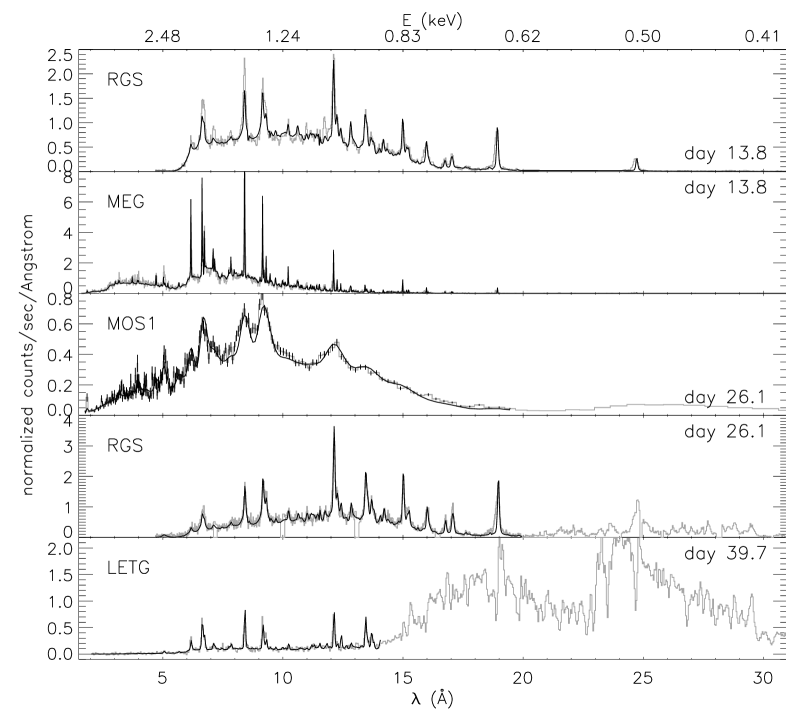
Figure 9.— Best-fit APEC models (from top to bottom) to the XMM-Newton/RGS and Chandra/MEG spectra on day 13.8 XMM-Newton/MOS1 and RGS spectra taken on day 26.1, and the Chandra/LETG spectrum taken on day 39.7. For day 26.1 the soft component longwards of 20 Å was excluded from the fit, and for day 39.7 the SSS spectrum had to be excluded.

Figure 10.— Elemental abundances relative to solar (Anders & Grevesse, 1989) from APEC fits to the spectra of days 13.8 and 26.1. Each grid point is the result of iterating all free parameters with the absolute abundance fixed at the respective grid value. Plotted are the changes in $\chi^{2}$ compared to the best fit. The dashed horizontal lines mark the 68-% and 95-% confidence ranges.

Because the spectra on days 13.8 and 26.2 are of such high quality, we investigate absolute abundances using these two datasets (Fig. 10). Although no hydrogen lines are present in the X-ray range, the absolute abundances can be determined from the strength of the continuum relative to the lines. The brightness of the continuum depends on the number of free electrons which, in an ionized plasma, scales with the hydrogen abundance. We thus need spectra with sufficient continuum emission. We step through a grid of (fixed) abundances and fit the remaining parameters to minimize $\chi^{2}$. In Fig. 10 we show the relative changes in $\chi^{2}$ for each grid point in comparison with the 68-% and 95-% confidence ranges (for 14 free parameters). While for day 13.8, solar abundances are preferred, the spectrum taken on day 26.1 suggests a somewhat lower metallicity, but from the confidence intervals one can see that their determination is highly uncertain. We therefore fix the absolute abundance at solar values and concentrate on the relative abundances.

The final model parameters are summarized in Table 5. From top to bottom we list $\log T$ and $\log VEM$ for each component, value of $N_{\rm H}$, and $\chi^{2}_{\rm red}$ with number of degrees of freedom ($dof$). The elemental abundances relative to solar (Anders & Grevesse, 1989) as determined from the day 13.8 dataset are given in Table 7 and have been used for all models.

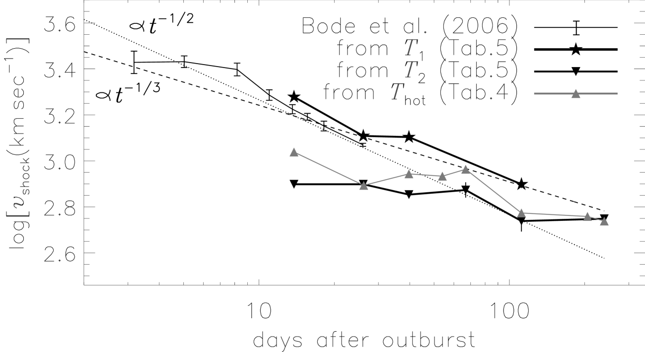
Figure 11.— Evolution of the shock velocity obtained from the temperatures found by Bode et al. (2006), from the temperatures of the first and second components of the APEC models (Table 5), and the highest temperatures measured from line ratios (Table 4). The dashed and dotted lines indicate the expected power law decay in an adiabatic plasma ($t^{-1/3}$) and in a radiatively cooling plasma ($t^{-1/2}$), respectively. The error bars are statistical errors. For additional systematic errors see §4.5.

In the same way as Bode et al. (2006) we compute shock velocities, $v_{\rm shock}$, from the temperatures of the first and second component of the APEC models (see Table 5), and from the highest temperatures found from line ratios (Table 4). In Fig. 11 we compare these results with those from Bode et al. (2006). The dotted and dashed lines indicate the expected evolution for a radiatively cooling plasma and an adiabatic plasma, respectively (Bode & Kahn, 1985). The velocities derived from $T_{1}$ of our 3-$T$ APEC models for days 13.8 and 26.1 are slightly higher than the Bode values. The reason is that the 1-$T$ models used by Bode et al. (2006) are an average of all temperature components, accounting for some of the cooler plasma that in our 3-$T$ models are accounted for by the two cooler components. The evolution of $T_{1}$ follows the same trend as observed by Bode et al. (2006). After day 26.2, the hottest component is much fainter, and $T_{1}$ is less certain. In Figs. 4 and 5 one can see that the continuum emission level is significantly lower than that seen in Figs. 2 and 3. Since the parameters of the hottest temperature component are dominated by the continuum, systematic uncertainties from background noise have a stronger effect, and the velocities derived from the hottest temperature components may be overestimated for the observations taken after day 26.1 (see §4.5).

The second plasma component is very similar to the values derived from the line ratios (Table 4), but these curves follow a different trend than the hottest component. For the observations of days 13.8 and 26.1, the line ratios yield much lower velocities than those from the APEC models. We attribute this difference to the stronger continuum observed for these two days. Since the continuum is dominated by the hottest plasma, the hottest temperature in the APEC models is driven by the continuum which, during the early observations, reflects a higher temperature than any of the emission lines can probe. Meanwhile, the emission lines can probe the structure of the temperature distribution better, and in the next section we describe an approach that focuses on a few selected emission lines.

4.3. Emission measure modeling

Table 6Comparison of line flux measurements with predictions for day 13.8

Iona	$\lambda$	$F_{\rm meas}^{b}$	$\frac{F_{\rm meas}}{F_{\rm pred}}^{c}$
N VI	28.79	543	$0.93\,\pm\,0.23$
N VII	24.78	1514	$1.03\,\pm\,0.04$
O VII	21.60	1200	$1.13\,\pm\,0.14$
O VII	22.10	686	$1.00\,\pm\,0.20$
O VIII	18.97	1871	$0.86\,\pm\,0.19$
Ne IX	13.45	358	$0.95\,\pm\,0.12$
Ne IX	13.70	183	$0.96\,\pm\,0.19$
Ne X	12.14	927	$0.99\,\pm\,0.07$
Mg XI	9.17	705	$1.03\,\pm\,0.08$
Mg XII	8.42	669	$0.99\,\pm\,0.03$
Si XIII	6.65	816	$1.05\,\pm\,0.05$
Si XIV	6.19	438	$0.94\,\pm\,0.03$
S XV	5.04	708	$1.10\,\pm\,0.15$
S XVI	4.73	245	$0.72\,\pm\,0.07$
Fe XVII	12.26	65.0	$1.13\,\pm\,0.61$
Fe XVII	15.02	448	$0.85\,\pm\,0.10$
Fe XVIII	14.21	216	$1.17\,\pm\,0.26$
Fe XX	12.83	69.8	$0.69\,\pm\,0.39$
Fe XX	12.85	97.7	$1.08\,\pm\,0.44$
Fe XXI	12.28	174	$0.96\,\pm\,0.39$
Fe XXII	11.77	92.5	$1.07\,\pm\,0.20$
Fe XXIII	10.98	69.6	$1.33\,\pm\,0.26$
Fe XXIII	11.74	99.8	$1.49\,\pm\,0.25$
Fe XXIV	11.17	46.8	$1.46\,\pm\,0.41$
Fe XXV	1.85	1045	$29.4\,\pm\,5.40$
Fe XXVI	1.78	$<145$	$<5.19$

$\bullet\ ^{a}$Lines used in deriving the mean EMD are given in bold face. $\bullet\ ^{b}$Fluxes from Table 3 in $10^{-14}$ erg cm^-2 s^-1, corrected for absorption assuming $N_{\rm H}=5\times 10^{21}$ cm^-2 $\bullet\ ^{c\,}$Predicted from the derived EMD, assuming constant pressure $\log P_{\rm e}=13.0$

Table 7Elemental abundances relative to solar

	day 13.8		day 111.7
	EMD model	APEC model	EMD model
correction factors
O	1.0	$0.77\,\pm\,0.03$	1.0
N	$6.94\,\pm\,0.44$	$7.12\,\pm\,0.70$	$7.54^{+12}_{-5}$
Ne	$1.39\,\pm\,0.11$	$0.68\,\pm\,0.03$	$1.36\,\pm\,0.16$
Mg	$2.29\,\pm\,0.08$	$1.06\,\pm\,0.03$	$1.91\,\pm\,0.70$
Si	$2.04\,\pm\,0.08$	$0.88\,\pm\,0.03$	$1.62\,\pm\,1.0$
S	$3.16\,\pm\,0.21$	$0.69\,\pm\,0.12$	–
Fe	$0.50\,\pm\,0.04$	$0.29\,\pm\,0.01$	$0.43\,\pm\,0.10$
relative to oxygen
$[$N/O$]$	$0.84\,\pm\,0.03$	$0.95\,\pm\,0.05$	$0.88^{+0.41}_{-0.47}$
$[$Ne/O$]$	$0.14\,\pm\,0.04$	$0.04\,\pm\,0.03$	$0.13\,\pm\,0.05$
$[$Mg/O$]$	$0.36\,\pm\,0.02$	$0.24\,\pm\,0.02$	$0.28\,\pm\,0.20$
$[$Si/O$]$	$0.31\,\pm\,0.02$	$0.16\,\pm\,0.02$	$0.21\,\pm\,0.42$
$[$S/O$]$	$0.50\,\pm\,0.03$	$0.17\,\pm\,0.08$	–
$[$Fe/O$]$	$-0.30\,\pm\,0.03$	$-0.50\,\pm\,0.03$	$-0.37\,\pm\,0.11$
relative to iron
$[$N/Fe$]$	$1.14\,\pm\,0.05$	$1.43\,\pm\,0.07$	$1.24\,\pm\,0.58$
$[$O/Fe$]$	$0.30\,\pm\,0.05$	$0.50\,\pm\,0.03$	$0.37\,\pm\,0.09$
$[$Ne/Fe$]$	$0.45\,\pm\,0.05$	$0.53\,\pm\,0.05$	$0.47\,\pm\,0.15$
$[$Mg/Fe$]$	$0.66\,\pm\,0.04$	$0.73\,\pm\,0.03$	$065\,\pm\,0.23$
$[$Si/Fe$]$	$0.61\,\pm\,0.04$	$0.65\,\pm\,0.04$	$0.58\,\pm\,0.35$
$[$S/Fe$]$	$0.80\,\pm\,0.05$	$0.67\,\pm\,0.12$	–

all values relative to Grevesse & Sauval (1998)

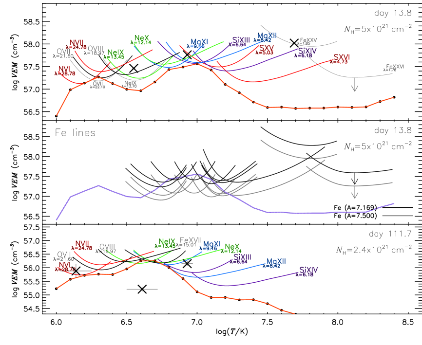
Figure 12.— Upper panel: Emission measure loci $L_{\lambda}(T)$, calculated for each line using Eq. 3 with line fluxes measured on day 13.8, and line emissivities assuming rescaled solar abundances (Grevesse & Sauval, 1998) using the scaling factors listed in the top part of Table 7. The black bullets, connected by a thick solid line indicate the mean emission measure distribution (EMD) yielding the best reproduction of the measured line fluxes. The loci for some lines that are not used to optimize the EMD are shown with light gray. The black X symbols indicate the results from 3-$T$ APEC models listed in Table 5 (see §4.2 and discussion in §4.4). Middle panel: Emission measure loci only for Fe lines (gray: assuming solar abundances, black: corrected by factor 0.46 times solar) and the best-fit EMD from the top panel in purple. The bulk of the lines demands a reduction of the Fe abundance, but the Fe xxv locus (top right curve) is then too high. The locus of Fe xxvi (far right curve) is an upper limit. The contribution function of H-like Fe xxvi above $10^{8}$ K is estimated by extrapolating from the data below $10^{8}$ K assuming the same shape as the H-like line of S xvi. Bottom panel: Same as top panel for line fluxes measured on day 111.7. The same elemental abundances are used. The black X symbols indicate the results from APEC models listed in Table 5.

We use the measured line fluxes listed in Table 3 (corrected for absorption; see below) in order to reconstruct a continuous mean emission measure distribution (EMD) as a function of temperature, i.e., $VEM(T)$. We assume a constant electron pressure of $\log(P_{\rm e})=13.0$ (in units K cm^-3), which is equivalent to a density $\log(n_{\rm e}[{\rm cm}^{-3}])\lesssim 7$, depending on temperature. While this assumption is more realistic than $\log(n_{\rm e})=0$ (as used for the APEC models) this is still very crude, however, we use only lines that are not density-sensitive such that the results do not depend on the assumed pressure.

We concentrate on the two simultaneous observations taken on day 13.8 because the combined Chandra and XMM-Newton data provide the largest coverage in lines and most reliable line flux measurements. Details of the method are described in Ness & Jordan (2008). A similar approach has been described by Ness et al. (2005). A continuous EMD is a more realistic representation than multi-temperature models, and it is a way to overcome the extreme simplification of assuming an isothermal plasma (e.g., Bode et al., 2006). We use Eq. 2 to compute line fluxes from a given EMD and compare the predicted fluxes to the measured fluxes. For Eq. 1 we assume the same ionization balance that Ness & Jordan (2008) used. The elemental abundances are relative to solar by Grevesse & Sauval (1998).

As a guide to construct a starting EMD we compute the so-called emission measure loci $L_{\lambda}(T)$, which are the ratios of the measured line fluxes, $f_{\lambda}$, and the line contribution functions, $G_{\lambda}(T)$ (Eq. 1), i.e.,

$$L_{\lambda}(T)=\frac{f_{\lambda}}{G_{\lambda}(T)}\,.$$ (3)

In Fig. 12 we show these loci for a set of lines selected on the grounds that the atomic physics are reliable and that the measured line fluxes (corrected for $N_{\rm H}=5\times 10^{21}$ cm^-2 for day 13.8 and $N_{\rm H}=2.4\times 10^{21}$ cm^-2 for day 111.7) are either not blended with other lines or are easy to deblend (see comments in Table 3). A few other lines are shown for comparison in light gray with the label at their minima. Since the line contribution functions $G_{\lambda}(T)$ scale with the elemental abundances (see Eq. 1), a reduction in abundances leads to an increase of $L_{\lambda}(T)$ at all temperatures and vice versa. Because most Fe lines are quite weak, difficult to measure, and are subject to less certain atomic physics because of the complex ion structures, we exclude all Fe lines from constraining the mean EMD.

To find a model that reproduces the selected line fluxes we construct an initial EMD by eye. We start with the envelope curve below the minima of all $L_{\lambda}(T)$ curves and make successive changes to the EMD and to the elemental abundances until the predicted line fluxes agree qualitatively with the measured values. We adjust only the abundances of elements that produce strong lines, except for oxygen. The oxygen line fluxes pose a constraint on the normalization, and all abundances are thus relative to oxygen. Since the line contribution functions are broader than 0.2 dex, no narrow features in the temperature distribution can uniquely be resolved, and we thus allow no features in the EMD that are narrower than the line contribution functions. We stress that with our approach we are determining only one possible representation of the true nature of the shocked plasma since Eq. 2 represents a Fredholm integral equation which is not uniquely solvable. However, Ness & Jordan (2008) pointed out that the determination of elemental abundances seems fairly robust against the precise form of the assumed mean emission measure distribution.

Once a reasonable model is found we fine-tune the model by iteration of the mean EMD, optimizing the predicted line fluxes using the method described by Ness & Jordan (2008). Based on the ratios of measured to predicted line fluxes for the best-fit models, we modify the abundances of elements where systematic discrepancies can be identified and repeat the fine-tuning of the EMD. In this way we consecutively approach a good representation of all lines included in the fit as well as some other lines that are not included.

The final model is indicated with the thick solid line in the top panel of Fig. 12. The best fit yields two peaks at $\sim 10^{7}$ K and $\sim 2\times 10^{6}$ K. The high-temperature regime is poorly determined because the only lines formed at temperatures above $\log T=7.5$ are those of Fe xxv and Fe xxvi. For the latter line we only have an upper limit to the flux. The use of these lines is limited by the unknown Fe abundance at this stage.

In the middle panel of Fig. 12 we show emission measure loci of ten Fe lines measured from the MEG and HEG spectra taken on day 13.8. The grey curves are the loci calculated with solar Fe abundance, and all loci around $\log T\sim 7$ need to be raised (yielding a reduction of the Fe abundance) in order to be consistent with the mean EMD derived from the other lines. If the Fe abundance is reduced by a factor 0.5 (black loci), the reproduction of the Fe lines improves significantly. Only, the Fe xxv line is not reproduced, yielding an underprediction by a factor of 30.

The excessively high Fe xxv flux in combination with the non-detection of the Fe xxvi line is difficult to explain. While the underestimated flux for Fe xxv could be fixed with more emission measure at high temperatures, such a modification demands a detectable flux of the Fe xxvi line. When increasing the emission measure only at temperatures where the Fe xxv lines are formed, the S xvi line is significantly overpredicted. We are confident that the Fe xxv emissivity function is not underestimated, as the two atomic data bases APEC and CHIANTI give consistent emissivities and it seems unlikely to us that both databases would give the wrong emissivities for such a relatively simple (He-like) ion.

Another possibility is that the underlying assumptions for the calculation of the predicted line fluxes for Fe xxv are incorrect. Our assumption of constant pressure $\log P=13$ implies that Fe xxv is formed in an environment of $\log n_{e}\sim 5-6$, thus a rather low density. However, in order to make a significant difference in the predicted Fe xxv lines the density would have to be in excess of $10^{16}$ cm^-3, and we reject this possibility (see also lower part of Table 4). The Fe xxv flux could be enhanced by resonant scattering into the line of sight if the plasma is not optically thin. This would only affect the resonance lines, and the Fe xxvi line would also have to be enhanced but it is not detected. While the emissivities used to compute the Fe xxv locus curve uses the combined emissivities from the resonance, intercombination, and forbidden lines, contributions from unresolved satellite lines are neglected. These can dominate the Fe xxv complex at temperatures below the peak formation temperature (i.e., at $\log T<7.8$; Oelgoetz & Pradhan 2001). Lastly, a number of non-equilibrium processes have significant effects on the Fe xxv complex (see Oelgoetz & Pradhan 2004). For example, recombination into excited states would enhance the Fe xxv lines at the expense of Fe xxvi and could explain the unusually high locus of the Fe xxv lines. While significant effects of recombination of Fe xxvi into Fe xxv violates the underlying assumption of collisional equilibrium, this does not necessarily imply that the other lines are also affected. Recombination affects only the ionization stages whose ionization energy is higher than the kinetic energy of the hottest plasma component. The energy required to ionize Fe xxv into Fe xxvi is 8.8 keV (equivalent to $10^{8}$ K), and that is higher than the hottest plasma component found from the APEC models of $\log T=7.69$ (Table 5). Meanwhile, the ionization temperature of Fe xxiv into Fe xxv is only 2.04 keV ($10^{7.38}$ K) which is clearly lower than the hottest plasma component, and Fe xxiv and Fe xxv can be considered to be in equilibrium. Also, S xvi and S xv are in equilibrium, since the ionization energy is 3.224 keV ($=10^{7.57}$ K). We therefore conclude that only Fe xxv and Fe xxvi might not be in equilibrium while all other lines are, and our underlying assumptions are valid for these lines.

In Table 6 we list the measured and predicted line fluxes for our best EMD for day 13.8 (Fig. 12), giving element, rest wavelength, measured fluxes (after deblending and correction for $N_{\rm H}=5\times 10^{21}$ cm^-2), and ratios of measurements and predictions. We assume a value of $N_{\rm H}$ that is lower than that found from the APEC models (Table 5) because we are unable to find an EMD model with that value that gives such good reproduction of all line fluxes. Also, with lower values of $N_{\rm H}$ we are having difficulties to find a good EMD model, and values as low as the interstellar value of $N_{\rm H}=2.4\times 10^{21}$ cm^-2 can be excluded. We note that the EMD modeling is not an ideal way to determine $N_{\rm H}$, and we refrain from determining a confidence range for $N_{\rm H}$ but consider it an uninteresting parameter, thus concentrating on the elemental abundances. We note that the chosen value of $N_{\rm H}$ is consistent with the total column density found by Bode et al. (2006).

In Table 7 we give the correction factors applied to the abundances. The EMD is scaled to reproduce the oxygen lines assuming solar O abundance (correction is 1.0), and the correction factors are thus equivalent to the respective abundances relative to solar. We also give the logarithmic abundances in the standard notation and list abundances relative to Fe (computed from the respective values relative to oxygen) in the bottom of Table 7. We determine the uncertainties of abundances by stepping through a grid of values, each time readjusting the EMD and computing a value of $\chi^{2}$ from the measured fluxes with their uncertainties for the selected lines. The listed uncertainties are derived from increases of $\chi^{2}$ by one, which in the case of a 1-parameter model would be the 1-$\sigma$ uncertainties. We note that our model is not a parameterized model.

In the absence of any hydrogen lines, absolute abundances can only be determined via the strength of the continuum relative to the lines (see above). Since the mean EMD is not well constrained at high temperatures, the shape of a continuum model predicted by the EMD disagrees with the observed spectrum. It is not possible to adjust the EMD without conflicts with some of the emission lines, and we thus refrain from determining absolute abundances with this method.

We apply the same approach using the line fluxes from other observations listed in Table 3, and show the results in the bottom panel of Fig. 12 for day 111.7. All emission measure values are significantly lower, and there is no indication for plasma hotter than $\log T=7$. The abundances are given in the last column of Table 6, and they are all consistent with those found on day 13.8. This conclusion also holds for the other datasets, although it is more difficult to distinguish between different EMD models. The reasons are lack of lines formed at low temperatures for the observations taken on days 26.1, 39.7, 54.0, and 66.9 and lack of lines formed at high temperatures for the observations taken after day 111.7. Also, some lines are blended with other nearby lines which can be disentangled with the Chandra HETGS, but not with the XMM-Newton RGS and Chandra LETGS.

In Fig. 13 we show the minima of the emission measure loci for all observed line fluxes using different plot symbols for each observation as explained in the legend. To guide the eye we connect the datapoints belonging to the same observations with solid and dotted lines in order that the evolution of the temperature structure can be identified. A similar plot has been presented by Schönrich & Ness (2008) who assumed the same value of $N_{\rm H}=2.4\times 10^{21}$ cm^-2 for all observations and solar abundances. They found significantly higher loci for the N and O lines for days 39.7 and 66.9 compared to all other observations. Since during the SSS phase these lines appeared on top of the SSS continuum, they concluded that these lines are formed within the outflow or are at least affected by the SSS radiation. We now use the new abundances from Table 7 and $N_{\rm H}=5\times 10^{21}$ cm^-2 for days 13.8 and 26.1 and $N_{\rm H}=2.4\times 10^{21}$ cm^-2 for the rest (see Table 5). The higher value of $N_{\rm H}$ for days 13.8 and 26.1 leads to higher loci of the low-temperature lines of O and N which are now consistent with those measured for day 39.7 and 66.9. In order to attribute these lines to either the outflow or the shock therefore requires accurate knowledge of the value of $N_{\rm H}$. But even with our improved measurements of $N_{\rm H}$ the situation remains ambiguous because, if the O and N lines observed on top of the SSS continuum are formed somewhere within the outflow, they might be subject to higher values of $N_{\rm H}$ as is suggestive from the shock plasma. This would increase the discrepancies again, and with these uncertainties, it may never be possible to decide whether these emission lines are formed in the outflow or in the shock.

At the other end of the temperature distribution, at $\log T>6.8$, a steady decrease of emission measure can be identified. The slope of the temperature distribution toward the highest temperatures seems to become steeper, indicating that the hot plasma is cooling rapidly, while below $\log T=6.8$ the line emission measures also decrease, but the slope remains about the same, and the cool component thus cools at a slower rate.

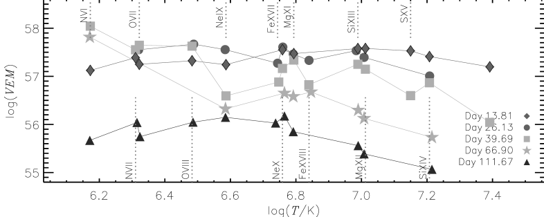
Figure 13.— Volume emission measures ($VEM$) at the peak formation temperature for selected strong lines, assuming the abundances listed in Table 7. The connecting lines guide the eye, but are not EMD models. The plot symbols indicate the time of observation after outburst according to the key in the bottom right legend. We use dark gray for observations taken before the SSS appeared, light gray for observations during the SSS phase and black for after the SSS spectrum had disappeared.

4.4. Comparison of models

While the APEC models introduced in §4.2 include all available atomic information, the line-based approach used in §4.3 has the advantage that only the most reliable information is selected. Less certain lines (e.g., lines with transitions involving higher principal quantum numbers) are discarded. In §4.3 the crude assumption of constant pressure is sufficient because only lines that are not density-sensitive are selected. The APEC model makes the even cruder assumption of a low-density plasma ($\log n_{e}=0$: Smith et al., 2001a), while density-sensitive lines are not excluded. However, most density-sensitive lines are weak. Another difference is the assessment of the goodness of a model. In our line-based approach the fitting yields best reproduction of measured line fluxes (taking line broadening into account), while with xspec the count rate in each spectral bin has to be reproduced. In cases where lines are present in the observed spectra that are missing in the atomic database, we can ignore them with the line-based approach, while with xspec the existing lines in the atomic database can be used to force an acceptable fit of these spectral regions. Furthermore, the individual emission lines contribute only to a few spectral bins such that negligence of emission lines is badly penalized compared to negligence of the continuum. On the other hand, the APEC models are much better suited to assess the hottest temperature component via the continuum, and the corresponding shock velocities can only be derived from the APEC models (see Fig. 11). For more discussion on line-based and global fitting approaches we refer to Ness (2006). We thus need both approaches for robust conclusions.

In the top panel of Fig. 12 we include the temperatures and volume emission measures of the three components derived from the 3-$T$ APEC models fitted to the spectra of day 13.8 for comparison with the mean EMD. All three components yield higher values of emission measure than the continuous EMD, because all emission from the smooth distribution of the EMD model is concentrated in only three isothermal components. The emission measure of the hottest component of the APEC model is much higher than in the EMD model. Since not enough emission lines are formed above $10^{7.5}$ K to constrain the EMD, the line-based approach is clearly inferior in this temperature regime, and the hottest component is driven by the continuum. We further find that only the lines that are formed at high temperatures are affected by recombination (see §4.3). The second temperature component of the APEC model coincides with the temperature of the hotter peak of the mean EMD. The third component is closer to the minimum between the two peaks of the mean EMD (see Fig. 12). The higher temperature in the APEC model could explain why the N abundance is higher than that derived from the EMD modeling. Since each temperature component is isothermal, the N lines are not as efficiently produced by the cool component, which has to be compensated by a higher N abundance in order to fit the N lines. We also note that the N vi line at 28.78 Å, which is clearly detected (see Table 3), is completely ignored by the APEC models but represents an important constraint on the EMD model. Finally, in the xspec fits we could not account for line broadening (see §4.2), while we used the line fluxes integrated over the entire profile for the EMD reconstruction method. We therefore regard the abundances of O and N derived from the EMD model as more reliable than the values derived from the APEC model.

For all models, we give only statistical uncertainties. Uncertainties from the atomic physics are not included and are a source of additional systematic uncertainty (§4.5). Since many lines with poorly-known atomic physics are included in the APEC models the systematic uncertainties of the APEC models are higher than those from the EMD models.

For comparison of the elemental abundances derived from the two approaches, we rescale those obtained in §4.2 because the reference abundances used in the APEC models are those by Anders & Grevesse (1989), while for the EMD reconstruction method we have used those by Grevesse & Sauval (1998). We rescale by a factor $(N_{\rm X}/N_{\rm O})_{\rm grev}/(N_{\rm X}/N_{\rm O})_{\rm and}$, where the subscripts ’grev’ and ’and’ denote the abundance ratios from Grevesse & Sauval (1998) and Anders & Grevesse (1989), respectively. The correction factors are 0.933, 1.23, 1.259, 1.259, 1.66, and 0.85 for N, Ne, Mg, Si, S, and Fe, respectively. In Table 7 all derived abundances are listed for comparison. While the abundance ratios relative to O are discrepant, those relative to Fe agree much better, except for N/Fe. We attribute these differences to the low formation temperatures of the N and O lines. We attribute these differences to the less certain N and O abundances derived from the APEC models that underestimate the amount of cool plasma (see above). We expect overestimated N and O abundances and possibly also Ne in the APEC model which explains that all abundances relative to O are lower in the APEC model compared to the EMD model. Since the N lines are formed at lower temperatures than the O lines, the N abundance is affected to a higher degree. The Fe lines are formed over a large range of temperatures and are therefore not as strongly affected, leading to the overall better agreement of all ratios relative to Fe. For the observation taken on day 111.7 only the EMD modeling yields some constraints on the elemental abundances, which demonstrates the strength of this approach over the spectral fitting.

4.5. Uncertainties

While the results from §2 are directly based on the observations, all results from this section, §4, depend on model assumptions which are described in §4.1. All error estimates given in this paper are statistical 1-$\sigma$ uncertainties which give the 68.3-per cent probability that fitting the same model to a new observation with the same instrumental setup results in parameters within the given uncertainty ranges. They thus only describe the precision of our measurements, but not the accuracy (sum of statistical and systematic uncertainties) which depends on the calibration of the observations but also on the choice of a model. For comparisons of measurements taken with the same instrument (given in Table 1), the systematic calibration uncertainties can be neglected but have to be kept in mind for absolute numbers and comparisons with different instruments (e.g. the flux evolution shown in Fig. 6). For line profiles (Fig. 7) and line ratios (Fig. 8), the cross-instrument calibration uncertainties are negligible.

For the flux measurements presented in Fig. 6, systematic uncertainties arise from the choice of band width which excludes a fraction of the total X-ray emission. Owing to the presence of the SSS spectrum between days 39.7 and 66.9, the contribution from emission between 11 and 38 Å to the shock emission can not be determined, yet the fraction of soft emission may be higher compared to before day 39.7. Attempts to determine this contribution from the xspec models failed because we have no constraints from observations because the much stronger SSS emission dominates at long wavelengths. We estimate that the systematic uncertainties on the Swift light curve shown in Fig. 6 are small, because the spectral shape hardly changes after day 100 (see Table 5), and the X-ray flux thus scales directly with the observed count rate. We note that systematic uncertainties from direct rescaling are smaller than the method of flux determination via model fitting to each individual Swift spectrum.

For the line shift measurements presented in Fig. 7 and §3.1, systematic uncertainties can arise from line blends and background noise, which affects the weaker lines more than stronger lines. For the measurement of line fluxes we have not accounted for uncertainties from choice of a source background (continuum) underneath the lines and from the line widths. Ness & Jordan (2008) found that the uncertainties in the line widths have less effect than the choice of continuum. For the line ratios presented in Fig. 8, additional systematic uncertainties from the continuum are less than 5 per cent if the continuum is assumed to be uncertain at the 20 per cent level.

For the model fits, the main sources of systematic uncertainty are the model assumptions and uncertainties in the atomic data. Both are difficult to quantify. The hottest temperature components of the 3-$T$ fits presented in Table 5 are driven by the continuum. The Fe xxv and Fe xxvi lines are the only strong lines formed at temperatures higher than $\sim 10^{7}$ K, and their absence in a model poses little resistance against an overestimated continuum temperature. For observations with weak continuum, arbitrarily high temperatures can thus result, and we give higher confidence to the temperatures of the hottest component determined from observations before day 39.7 (see Table 5). In view of these large systematic uncertainties of the later observations, the trends of shock velocities plotted in Fig. 11 are only reliable for the early observations. Since the apparent $t^{-1/3}$ trend that is suggestive from the values derived for day 39.7 and 111.7 is based on the higher temperature estimates compared to the expected $t^{-1/2}$ trend, the conclusion of adiabatic cooling instead of the theoretically expected radiative cooling has to be treated with caution.

The uncertainties in elemental abundances resulting from the emission measure modeling (Table 7) are extremely difficult to quantify. They mainly depend on the uncertainties in the line flux measurements and the uncertainties in the determination of the mean EMD. Ness & Jordan (2008) found from comparison to independent analyses of the same spectrum by Sanz-Forcada et al. (2003) that the abundances are quite robust against changes in the assumed mean EMD. Since the abundance determination is based on strong lines originating from few-electron ions (thus well-known atomic physics), we are confident that the given uncertainties that are based on the measurement uncertainties of line fluxes are realistic.

5. Discussion

The X-ray grating spectra give the deepest insight into the properties of the shocked plasma. With 12 grating observations we can follow the changes in the X-ray flux and plasma temperature, and we have determined the elemental abundances from the emission lines. The X-ray flux can directly be integrated over the spectrum without the need of a model and can thus be considered an observed quantity. We are further able to determine temperatures independently from line flux ratios and from spectral models, and we are able to detect different temperature components. The ability to measure line fluxes also enables us to pursue two independent approaches to determine the elemental abundances, yielding robust results. We confirm that the underlying assumptions are generally satisfied, but we find evidence for recombination in the Fe xxv He-like triplet lines and the Fe xxvi lines. Since these are the only ions whose ionization energy exceeds the kinetic energy of the hottest plasma component, we regard the assumptions discussed in §4 valid for all other lines.

We observe a power-law decay in X-ray flux, and the power-law index changes from $\alpha=-5/3$ before day $\sim 70$ to $\alpha=-8/3$ during the later evolution (see Fig. 6). While the $t^{-5/3}$ decay is predicted for a radiatively cooling shock traversing an $r^{-2}$ density distribution, the change to a t^-8/3 decay at late times cannot be simply explained. However, note that Vaytet et al. (2007) found that in some circumstances the forward shock could decelerate faster than the standard cooled momentum-conserving models predict. In addition, it is interesting to note that a steeper decay may result from the breakout of the forward shock into a lower density environment when it reaches the edge of the red giant wind re-established in the 21 year interval between explosions. Indeed, simple calculations suggest that this breakout may happen around the time of the apparent break in decay curves (see, e.g., Mason et al. 1987; O’Brien et al. 1992). One possible problem with this conclusion however is that the immediate post-shock temperature increases, rapid adiabatic expansion of the emitting material will likely lead to a drop in the temperature derived from fits to the X-ray spectra, which does not seem to be the case. Furthermore, Bode et al. (2008) conclude from the apparent early onset of the adiabatic expansion phase in the forward shock that shock breakout will occur much later than realized from X-ray observations that in 1985 started only at 55 days post-outburst.

The two peaks in the emission measure distribution (see Fig. 12) could represent the forward and reverse shocks, where the cooler component would be the reverse shock. But according to models by Bode & Kahn (1985), the reverse shock may not be a significant source of X-ray emission at this time. Alternatively, the two temperature regimes could relate to forward shocks propagating into two distinct circumstellar density regimes, e.g., denser equatorial regions and less dense polar regions as suggested by VLBA/EVN and HST observations (Bode et al., 2007; O’Brien et al., 2006). More realistic hydrodynamic modelling is needed, and this is underway (see Vaytet et al., 2007).

In several Classical Novae, e.g., V382 Vel, X-ray spectra similar to those of the late evolution in RS Oph have been obtained after the nova had turned off and were attributed to the ejecta that are radiatively cooling (Ness et al., 2005). It is thus possible that the cooler component observed after day 70 originates from the expanding ejecta, while the early hot and cool components represent the shock emission.

5.1. Elemental Abundances

For our EMD models and multi-temperature fits, we have assumed uniform abundances throughout the X-ray emitting plasma. If the relative contributions from each component to the observed X-ray emission change with time and their compositions are significantly different, then in principle, changes in observed abundances derived from different observations are possible. However, the relative abundances obtained for days 13.8 and 111.7 do not differ significantly, and we conclude that no signs of changes in the composition are detectable. We therefore focus on our measurements for the best dataset taken on day 13.8. There are several issues for which the accurate determination of elemental abundances is of interest. The composition of the WD can be used as an argument whether or not RS Oph will explode as a canonical SN Ia. The WD may be near the Chandrasekhar limit, because of the short recurrence time scale, but if the WD consists of too many heavy nuclei (Mg, Ne rather than C, O), the amount of available nuclear binding energy is not sufficient to totally disrupt the WD. Note that it is the explosions of CO WDs that best fit the observations of SN Ia (Leibundgut, 2000; Hillebrandt & Niemeyer, 2000).

Since hydrogen is fully ionized in X-ray emitting plasma no H lines can be observed, and we cannot determine absolute abundances. In both of our approaches the attempt to determine absolute abundances from the strength of the continuum relative to the lines leads to ambiguous results, and we thus focus on relative abundances.

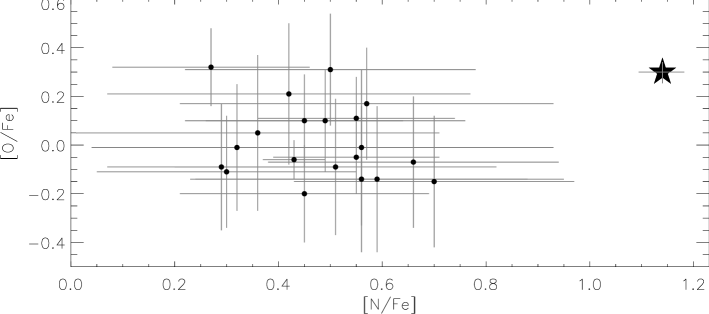
Figure 14.— Photospheric abundance ratios of 20 M giants given by Smith & Lambert (1985, 1986). The star symbol is our measurement for RS Oph as listed in Table 7. Uncertainties are given by gray error bars.

CNO-cycled material
There is no doubt, from both of our approaches, that nitrogen is overabundant. This points to CNO-cycled material, which could have been produced during the outburst. However, the companion is a red giant and is as such likely overabundant in nitrogen as well (see Fig. 14 and Smith & Lambert, 1985, 1986; Schmitt & Ness, 2002). The accreted material on the WD is thus already N-enhanced (Snijders, 1987a), as is the wind into which the ejecta run. In addition, nuclear burning during the outburst can contribute with more CNO-cycled material. Furthermore, N-enhanced material from previous outbursts may also contribute to the X-ray emitting plasma. Note that Walder et al. (2008) have determined from theoretical models that the ejecta are dominated by the RG material. In Fig. 14 we show the N abundance measurements of 20 M giants presented by Smith & Lambert (1985, 1986) versus their O measurements. The star symbol indicates our result for RS Oph, and it is clearly higher than any of the M giants, while the O abundance is consistent with most of the M stars. The comparison with other M giants thus suggests that CNO-processed material may have been added by the outburst. In support of this, the N/O abundance ratio derived from our two approaches is roughly similar to the value determined by Schönrich & Ness (2008) ($[$N/O$]=0.7$), who determined the ratio from the line column densities in the SSS spectra. Our result is also consistent with the abundance measurements by Contini et al. (1995) which yield an abundance ratio of $[$N/Fe$]=1.18$. The photospheric abundance measurements of the RS Oph secondary presented by Pavlenko et al. (2008) yield $[$N/Fe$]=0.9$ which can be compared to our abundance ratio $[$N/Fe$]=1.14$. This is lower than either our value or that determined by Schönrich & Ness (2008) ($[$N/Fe$]=1.0$ under the assumption of $[$O/Fe$]=0.3$), suggesting that the outburst has added about 20-40% of nitrogen into the X-ray detected material. We note that $[$N/Fe$]$ as derived by Pavlenko et al. (2008) is higher than any of the values plotted in Fig. 14. This indicates that the secondary in the RS Oph system is not a typical M giant which may be caused by the fact that the RS Oph secondary has lost significant amounts of material from its outer envelope during accretion to the WD.

If the material was CNO cycled, then we would expect it to be underabundant in carbon (see, e.g., Schmitt & Ness, 2002), but all carbon lines are at wavelengths where strong effects by interstellar and circumstellar absorption dominate. Moreover, uncertainties in $N_{\rm H}$ propagate to large uncertainties in any line fluxes or upper limits of the C lines (see Table 3). For any quantitative assessment of CNO burning, the carbon abundance is essential (Drake, 2003).

Nelson et al. (2008) discussed the carbon abundances and obtained an underabundance of C/N by a factor of 0.001 in order to explain the absence of the C vi K-shell absorption edge in the SSS spectra at 25.37 Å. This is much lower than the C/N abundance ratio of 0.05 that one derives from the $[$C$]=-0.4$ and $[$N$]=+0.9$, estimated by Pavlenko et al. (2008) for the secondary. Strong carbon lines were also observed in the IUE spectra by Shore et al. (1996). The absence of the C vi edge is not sufficient evidence for a C underabundance because other high-ionization absorption edges are also absent in the SSS spectra of RS Oph. For example, the ionization edges of O viii at 14.23 Å, O vii at 16.77 Å, N vii at 18.50 Å, and N vi at 22.457 Å are not present although these elements are not underabundant (see figs. 3 and 4 in Ness et al. 2007 and figs. 8 and 9 in Nelson et al. 2008). Since Ness et al. (2007) measured considerable blue shifts in the absorption lines observed during the SSS phase of RS Oph, the shell around the WD must be expanding with high velocities. While Nelson et al. (2008) found no blue-shifts in the same lines, they quote high velocities derived from line shifts of emission lines of C vi Ly series lines, however, without the presence of the Ly$\alpha$ line (Table 3). For an environment with high expansion velocities, the absorption edges may be washed out by the expansion. We therefore argue that without measurements of emission line fluxes of carbon, the C abundance cannot be determined from the X-ray spectra. Finally, a C/N abundance of 0.001 is far too low for any material that has undergone CNO cycle processing. The large N abundance requires some processing back to C (Starrfield et al., 2007).

$\alpha$ elements ($Z<22$)
The abundances of the $\alpha$ elements Ne, Mg, Si, S are significantly higher than O and Fe using both approaches. We use O as the reference element for our analysis, and our Ne/O abundance ratio is consistent the value found from IR observations by Evans et al. (2007b). This indicates that either Ne is overabundant or O is underabundant. Contini et al. (1995) found significant underabundance of O/H and of Ne/H of $\sim 10$% solar. We also list the ratios relative to Fe in Table 7. The abundance determinations by Contini et al. (1995) also yield high abundance ratios of $[$Mg/Fe$]=0.73$ and $[$Si/Fe$]=0.86$, which are roughly consistent with our results. Since Fe is neither produced nor destroyed in the outburst, we argue that all $\alpha$ elements are overabundant in the X-ray emitting plasma. Since we determined these values with two independent approaches using spectra with strong lines of relatively simple ions with well-known atomic data, we regard these results as reliable.

There are three possible explanations: (1) the $\alpha$ elements were produced during the outburst, (2), the composition of the secondary, which provides the accreted material and dominates the composition of the stellar wind, is overabundant in these elements (3) WD core material is enriched in the $\alpha$ elements, and that material has been mixed into the outflowing material.

(1) The production of $\alpha$ elements via nuclear burning requires high temperatures and densities. While the required temperatures are likely reached during the TNR, the densities are too low in order to produce significant amounts of $\alpha$ elements, even if the WD mass is near the Chandrasekhar mass.

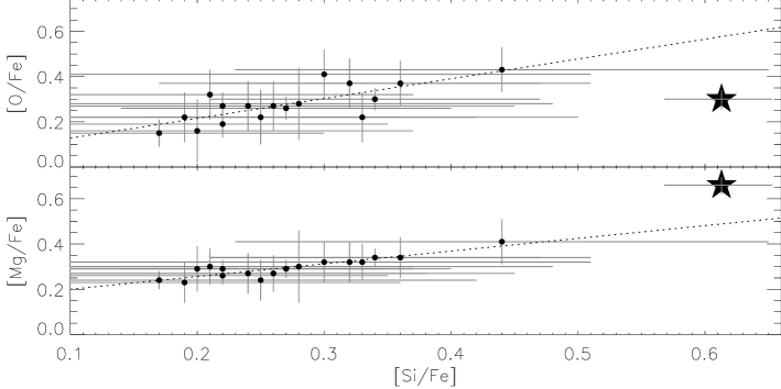
Figure 15.— Photospheric abundance ratios (relative to solar by Grevesse & Sauval 1998) of 17 M giants given by Rich et al. (2007). The star symbol is our measurement for RS Oph as listed in Table 7. Uncertainties are given by gray error bars.

(2) Direct abundance measurements of $\alpha$ elements for the secondary are not available, and Pavlenko et al. (2008) only determined Fe, C, and N abundances. Rich et al. (2007) measured photospheric abundances for 17 M giants in the inner bulge of the galaxy from IR spectroscopy. In Fig. 15 we show their abundances of $[$Si/Fe$]$ versus $[$O/Fe$]$ (top) and versus $[$Mg/Fe$]$ (bottom), relative to Grevesse & Sauval (1998). All M giants are overabundant in Si, O and Mg. Stars with a higher Si abundance are also higher in Mg and O, indicating different concentrations of the ashes of He shell flashes, probably due to different stellar ages. Our Si and Mg abundances for RS Oph are significantly higher than any of the M giants in the sample, but the O abundance is not higher. The bottom panel of Fig. 15 shows that our value is significantly higher in both elements than any of the M giants in the sample, and the concentration of all $\alpha$-elements could be higher. Since the outer envelope of the RS Oph secondary has been stripped away and accreted by the WD, higher abundances of all elements produced by He-burning can be expected. The surface composition may resemble that of the inner regions of normal M giants. Meanwhile, the O abundance could reflect a balance between a higher O abundance produced by He burning and a lower O abundance in material that has a higher concentration of CNO processed material as evident from Fig. 14. Our measurements can thus reflect the composition of the accreted material.

(3) If direct abundance measurements of the $\alpha$ elements of the secondary are different from our values, then the only remaining possibility would be that the WD contributes significantly to the composition of the observed plasma. The composition of the WD is dominated by elements that have been produced in the progenitor star. In order to be observable, WD material has to be dredged up and mixed into the outflowing material. While this is possible, no observations have so far revealed any signatures of WD material in the emitting regions of RS Oph.

5.2. Is RS Oph a SN Ia progenitor?

There is some speculation that RS Oph is a SN Ia progenitor. The short recurrence time scale suggests that the underlying WD is of high mass, possibly near the Chandrasekhar limit (e.g., Dobrzycka & Kenyon, 1994; Shore et al., 1996; Fekel et al., 2000). Hachisu & Kato (2001) reported a high-mass WD of $\sim 1.35\,\pm\,0.01$ M_⊙ (for both, high- and low-metallicity models), but their modelling neglects the environment and is not realistic. An even higher WD mass was estimated by Sokoloski et al. (2006), and Hachisu et al. (2007) also found that the WD is growing in mass. According to their estimated growth rate, the Chandrasekhar limit would be reached in a few times $10^{5}$ years.

ONe WDs do not provide enough nuclear binding energy (see, e.g., total binding energy calculations by Gamezo et al. 2003 or Calder et al. 2007), and when reaching the Chandrasekhar mass limit, they implode in a core collapse without an explosion. The explosion models of SN Ia predict that the WD has to be a CO WD for the supernova to be a canonical Ia explosion. However, the WD composition is not unambiguously determined.

A strong argument against RS Oph being a SN Ia progenitor is the large amount of hydrogen and helium in the system (e.g. Evans et al., 2007a) that has to be removed before the WD reaches the Chandrasekhar limit in order for the SN Ia outburst to be consistent with observations of hydrogen-deficiency (Filippenko, 1997). While the secondary loses hydrogen during the evolution of accretion and repeated outbursts, it would have to be considered too much of a coincidence if all the hydrogen is consumed in nova outbursts at the same time as the Chandrasekhar limit is reached. Considering these points, we believe that it is unlikely that RS Oph is a SN Ia progenitor.

6. Summary and Conclusions

The high-resolution X-ray spectra of the 2006 outburst of RS Oph provide unique insights into the properties and evolution of the outburst. The properties are best determined from the dataset taken on day 13.8. At this time of the evolution the nova was brightest in hard X-rays, and we have the best coverage with almost simultaneous Chandra and XMM-Newton observations. From these observations we have derived the elemental abundances with an overabundance of N, Ne, Mg, Si, and S, relative to Fe, indicating that this material has undergone CNO burning and He burning, respectively. Both processes can occur in the RG companion star, and our observations could reflect the donor material. CNO burning also occurs during the outburst, and by comparison of our results with direct measurements of the N abundance for the secondary by Pavlenko et al. (2008), we estimate that about 20-40% of the nitrogen could have been produced during the outburst. Meanwhile, no $\alpha$ elements can be produced during the outburst, but the underlying WD might be enriched in $\alpha$ elements.

We find Mg and Si significantly higher than in any M giant in the sample by Rich et al. (2007) which can either be explained by the RG being different from other M giants, or WD material has been dredged up during the outburst and mixed into the ejecta. Similarly high values have been found by Contini et al. (1995). Since the secondary has likely been stripped off it’s outer layers by mass loss onto the WD which has then been ejected during the outburst, the composition of the ejecta may be sampling deeper layers of the M giant companion as compared to the photospheric composition of normal M giants. In order to determine whether WD material is observed, direct measurements of the Mg and Si abundance in the photosphere of RG are needed for comparison.

We also determined the evolution of the temperature structure. The early observations show both a hot and a relatively cooler plasma component, while the later observations only display a cool component. Both components decay with time. Before day $\sim 70$, while the plasma is dominated by the hot component, the decay rate is slower than later in the evolution. The early decay rate is consistent with a radiatively cooling plasma while the later evolution can be explained by the expansion of the ejecta. The temperature evolution derived from models are consistent with radiative cooling of the hot component.

While it has been suggested that the WD is close to the Chandrasekhar limit, we note that there is currently too much hydrogen in the system for a supernova explosion to satisfy the spectroscopic features of a Ia explosion (Filippenko, 1997). The hydrogen and helium will have to be removed before the Chandrasekhar limit is reached. Further, the underlying WD has to be a CO WD, but the composition of the WD is difficult to determine since WD material has to be dredged up and ejected. Our abundance analysis suggests that this may be the case, but the composition of the accreted material is not well-enough known for solid conclusions at this time.

.1. Statistics

Some of the spectra are sufficiently bright for standard $\chi^{2}$ minimization, while others are extremely faint, and low-count statistics, as recommended by Cash (1979), have to be applied. According to Wilks theorem (Wilks, 1938), the Maximum Likelihood (ML) technique converges to the $\chi^{2}$ statistics in the high-count limit, and we thus apply the ML technique to all observations. The likelihood is defined as

$${\cal L}=-2\sum_{i=1}^{N}(n_{i}\ln m_{i}-m_{i})$$ (1)

with $n_{i}$ being an observation and $m_{i}$ a model, both defined on the same grid of $N$ bins. According to Wilks theorem ${\cal L}$ serves as a goodness criterion in an equivalent way as $\chi^{2}$, but it is derived from the Poissonian probability distribution function (PDF) rather than a Gaussian PDF. In order to conserve the Poissonian nature of the data, the instrumental background must not be subtracted. Instead, the model has to be added to the background for comparison with the raw data, because the sum of two Poissonian statistics is Poissonian, while the difference is not (Cash, 1979).

To assess the statistical uncertainty ranges of each parameter in a multi-parameter model we compute the curvatures of the likelihood at the respective best-fit values from the second derivatives. In order to assess the correlated uncertainties, we also compute mixed derivatives, thus the full Hessian matrix which, for $n$ free parameters, is an $n\times n$ matrix with the partial second derivatives of the likelihood curve, ${\cal L}={\cal L}(A_{i},A_{j})$,

$$H_{i,j}=\frac{\partial{\cal L}^{2}}{\partial A_{i}\partial A_{j}}$$ (2)

where $A_{i}$ and $A_{j}$ represent two free parameters with $i$ and $j$ ranging from 1 to $n$. We determine Eigenvectors, $EV_{i}(A_{j})$ and Eigenvalues, $ev(A_{j})$, and compute the correlated uncertainties from

$$\Delta A_{j}^{2}=\Delta{\cal L}\sum_{i=1}^{3}\frac{EV_{i}(A_{j})^{2}}{ev(A_{j})}$$ (3)

with $\Delta{\cal L}=2.3$ and $\Delta{\cal L}=3.53$ for 1-$\sigma$ uncertainties in the cases of two and three free parameters, respectively (Strong, 1985). Uncorrelated errors can be computed by setting all off-diagonal elements to zero before computing Eigenvectors and -values.

References

- Anders & Grevesse (1989) Anders, E., & Grevesse, N. 1989, Geochimica et Cosmochimica Acta, 53, 197
- Andrea et al. (1994) Andrea, J., Drechsel, H., & Starrfield, S. 1994, A&A, 291, 869
- Arnaud (1996) Arnaud, K. A. 1996, in Astronomical Society of the Pacific Conference Series, Vol. 101, Astronomical Data Analysis Software and Systems V, ed. G. H. Jacoby & J. Barnes, 17
- Blumenthal et al. (1972) Blumenthal, G. R., Drake, G. W. F., & Tucker, W. H. 1972, ApJ, 172, 205
- Bode et al. (2007) Bode, M. F., Harman, D. J., O’Brien, T. J., Bond, H. E., Starrfield, S., Darnley, M. J., Evans, A., & Eyres, S. P. S. 2007, ApJL, 665, L63
- Bode & Kahn (1985) Bode, M. F., & Kahn, F. D. 1985, MNRAS, 217, 205
- Bode et al. (2006) Bode, M. F., O’Brien, T. J., Osborne, J. P., Page, K. L., Senziani, F., Skinner, G. K., Starrfield, S., Ness, J.-U., Drake, J. J., Schwarz, G., Beardmore, A. P., Darnley, M. J., Eyres, S. P. S., Evans, A., Gehrels, N., Goad, M. R., Jean, P., Krautter, J., & Novara, G. 2006, ApJ, 652, 629
- Bode et al. (2008) Bode, M. F., Osborne, J. P., Page, K. L., Beardmore, A. P., O’Brien, T. J., Ness, J.-U., Starrfield, S., Skinner, G., Darnley, M. J., Drake, J. J., Evans, A., Eyres, S. P. S., Krautter, J., & Schwarz, G. 2008, in RS Ophiuchi (2006) and the recurrent nova phenomenon, ed. A. Evans, M.F. Bode, and T.J. O’Brien (Astronomical Society of the Pacific Society Conference Series), in press
- Calder et al. (2007) Calder, A. C., Townsley, D. M., Seitenzahl, I. R., Peng, F., Messer, O. E. B., Vladimirova, N., Brown, E. F., Truran, J. W., & Lamb, D. Q. 2007, ApJ, 656, 313
- Cash (1979) Cash, W. 1979, ApJ, 228, 939
- Contini et al. (1995) Contini, M., Orio, M., & Prialnik, D. 1995, MNRAS, 275, 195
- Dobrzycka & Kenyon (1994) Dobrzycka, D., & Kenyon, S. J. 1994, AJ, 108, 2259
- Drake (2003) Drake, J. J. 2003, ApJ, 594, 496
- Drake et al. (2008) Drake, J. J., Laming, M., Ness, J. U., & Starrfield, S. 2008, ApJ, in press
- Evans et al. (2007a) Evans, A., Kerr, T., Yang, B., Matsuoka, Y., Tsuzuki, Y., Bode, M. F., Eyres, S. P. S., Geballe, T. R., Woodward, C. E., Gehrz, R. D., Lynch, D. K., Rudy, R. J., Russell, R. W., O’Brien, T. J., Starrfield, S. G., Davis, R. J., Ness, J.-U., Drake, J., Osborne, J. P., Page, K. L., Adamson, A., Schwarz, G., & Krautter, J. 2007a, MNRAS, 374, L1
- Evans et al. (2007b) Evans, A., Woodward, C. E., Helton, L. A., Gehrz, R. D., Lynch, D. K., Rudy, R. J., Russell, R. W., Kerr, T., Bode, M. F., Darnley, M. J., Eyres, S. P. S., Geballe, T. R., O’Brien, T. J., Davis, R. J., Starrfield, S., Ness, J.-U., Drake, J., Osborne, J. P., Page, K. L., Schwarz, G., & Krautter, J. 2007b, ApJL, 663, L29
- Fekel et al. (2000) Fekel, F. C., Joyce, R. R., Hinkle, K. H., & Skrutskie, M. F. 2000, AJ, 119, 1375
- Filippenko (1997) Filippenko, A. V. 1997, ARAA, 35, 309
- Gabriel & Jordan (1969) Gabriel, A. H., & Jordan, C. 1969, MNRAS, 145, 241
- Gallagher & Starrfield (1978) Gallagher, J. S., & Starrfield, S. 1978, ARAA, 16, 171
- Gamezo et al. (2003) Gamezo, V. N., Khokhlov, A. M., Oran, E. S., Chtchelkanova, A. Y., & Rosenberg, R. O. 2003, Science, 299, 77
- Gehrz et al. (1998) Gehrz, R. D., Truran, J. W., Williams, R. E., & Starrfield, S. 1998, PASP, 110, 3
- Grevesse & Sauval (1998) Grevesse, N., & Sauval, A. J. 1998, Space Science Reviews, 85, 161
- Hachisu & Kato (2001) Hachisu, I., & Kato, M. 2001, ApJ, 558, 323
- Hachisu et al. (2007) Hachisu, I., Kato, M., & Luna, G. J. M. 2007, ApJ, 659, L153
- Hillebrandt & Niemeyer (2000) Hillebrandt, W., & Niemeyer, J. C. 2000, ARAA, 38, 191
- Hirosawa et al. (2006) Hirosawa, K., Narumi, H., Kanai, K., & Renz, W. 2006, Central Bureau Electronic Telegrams, 399, 1 (2006). Edited by Green, D. W. E., 399, 1
- Hjellming et al. (1986) Hjellming, R. M., van Gorkom, J. H., Seaquist, E. R., Taylor, A. R., Padin, S., Davis, R. J., & Bode, M. F. 1986, ApJL, 305, L71
- Jose & Hernanz (1998) Jose, J., & Hernanz, M. 1998, ApJ, 494, 680
- Kahabka & van den Heuvel (1997) Kahabka, P., & van den Heuvel, E. P. J. 1997, ARA&A, 35, 69
- Kashyap & Drake (2000) Kashyap, V., & Drake, J. J. 2000, Bulletin of the Astronomical Society of India, 28, 475
- Landi et al. (2006) Landi, E., Del Zanna, G., Young, P. R., Dere, K. P., Mason, H. E., & Landini, M. 2006, ApJS, 162, 261
- Leibundgut (2000) Leibundgut, B. 2000, AAPR, 10, 179
- Mason et al. (1987) Mason, K. O., Córdova, F. A., Bode, M. F., & Barr, P. 1987, in RS Ophiuchi (1985) and the Recurrent Nova Phenomenon, 167
- Mazzotta et al. (1998) Mazzotta, P., Mazzitelli, G., Colafrancesco, S., & Vittorio, N. 1998, A&AS, 133, 403
- Nelson et al. (2008) Nelson, T., Orio, M., Cassinelli, J. P., Still, M., Leibowitz, E., & Mucciarelli, P. 2008, ApJ, 673, 1067
- Ness (2006) Ness, J.-U. 2006, Advances in Space Research, 38, 1494
- Ness et al. (2003a) Ness, J.-U., Brickhouse, N. S., Drake, J. J., & Huenemoerder, D. P. 2003a, ApJ, 598, 1277
- Ness et al. (2004) Ness, J.-U., Güdel, M., Schmitt, J. H. M. M., Audard, M., & Telleschi, A. 2004, A&A, 427, 667
- Ness & Jordan (2008) Ness, J.-U., & Jordan, C. 2008, ArXiv 0711.3805, 711, MNRAS, in press
- Ness et al. (2001) Ness, J.-U., Mewe, R., Schmitt, J. H. M. M., Raassen, A. J. J., Porquet, D., Kaastra, J. S., van der Meer, R. L. J., Burwitz, V., & Predehl, P. 2001, A&A, 367, 282
- Ness et al. (2003b) Ness, J.-U., Schmitt, J. H. M. M., Audard, M., Güdel, M., & Mewe, R. 2003b, A&A, 407, 347
- Ness et al. (2007) Ness, J.-U., Starrfield, S., Beardmore, A., Bode, M. F., Drake, J. J., Evans, A., Gehrz, R., Goad, M., Gonzalez-Riestra, R., Hauschildt, P., Krautter, J., O’Brien, T. J., Osborne, J. P., Page, K. L., Schönrich, R., & Woodward, C. 2007, ApJ, 665, 1334
- Ness et al. (2006) Ness, J.-U., Starrfield, S., Drake, J. J., Orio, M., Bode, M. F., O’Brien, T. J., Davis, R. J., Osborne, J., Page, K. L., Schwarz, G., Krautter, J., Evans, A., Eyres, S. P. S., Gehrz, R., & Woodward, C. 2006, IAUC, 8683, 2
- Ness et al. (2005) Ness, J.-U., Starrfield, S., Jordan, C., Krautter, J., & Schmitt, J. H. M. M. 2005, MNRAS, 364, 1015
- Ness et al. (2008) Ness, J.-U., Starrfield, S., van Rossum, D. R., & Schönrich, R. 2008, in RS Ophiuchi (2006) and the recurrent nova phenomenon, ed. A. Evans, M.F. Bode, and T.J. O’Brien (Astronomical Society of the Pacific Society Conference Series), in press
- Ness & Wichmann (2002) Ness, J.-U., & Wichmann, R. 2002, Astronomische Nachrichten, 323, 129
- O’Brien et al. (1992) O’Brien, T. J., Bode, M. F., & Kahn, F. D. 1992, MNRAS, 255, 683
- O’Brien et al. (2006) O’Brien, T. J., Bode, M. F., Porcas, R. W., Muxlow, T. W. B., Eyres, S. P. S., Beswick, R. J., Garrington, S. T., Davis, R. J., & Evans, A. 2006, Nature, 442, 279
- Oelgoetz & Pradhan (2001) Oelgoetz, J., & Pradhan, A. K. 2001, MNRAS, 327, L42
- Oelgoetz & Pradhan (2004) —. 2004, MNRAS, 354, 1093
- Osborne et al. (2008) Osborne, J. P., Page, K. L., Beardmore, A. P., Goad, M. R., Bode, M. F., O’Brien, T. J., Starrfield, S., Ness, J.-U., Krautter, J., Schwarz, G., Burrows, D. N., Gehrels, N., Drake, J. J., & Eyres, S. P. S. 2008, submitted to ApJ
- Pavlenko et al. (2008) Pavlenko, Y. V., Evans, A., Kerr, T., Yakovina, L., Woodward, C. E., Lynch, D., Rudy, R., Pearson, R. L., & Russel, R. W. 2008, A&A, accepted
- Rich et al. (2007) Rich, R. M., Origlia, L., & Valenti, E. 2007, ApJL, 665, L119
- Sanz-Forcada et al. (2003) Sanz-Forcada, J., Brickhouse, N. S., & Dupree, A. K. 2003, ApJS, 145, 147
- Schmitt & Ness (2002) Schmitt, J. H. M. M., & Ness, J.-U. 2002, A&A, 388, L13
- Schmitt & Ness (2004) —. 2004, A&A, 415, 1099
- Schönrich & Ness (2008) Schönrich, R., & Ness, J.-U. 2008, in RS Ophiuchi (2006) and the recurrent nova phenomenon, ed. A. Evans, M.F. Bode, and T.J. O’Brien (Astronomical Society of the Pacific Society Conference Series), in press
- Shore et al. (1996) Shore, S. N., Kenyon, S. J., Starrfield, S., & Sonneborn, G. 1996, ApJ, 456, 717
- Smith et al. (2001a) Smith, R. K., Brickhouse, N. S., Liedahl, D. A., & Raymond, J. C. 2001a, ApJl, 556, L91
- Smith et al. (2001b) Smith, R. K., Brickhouse, N. S., Liedahl, D. A., & Raymond, J. C. 2001b, in Astronomical Society of the Pacific Conference Series, Vol. 247, Spectroscopic Challenges of Photoionized Plasmas, ed. G. Ferland & D. W. Savin, 161
- Smith & Lambert (1985) Smith, V. V., & Lambert, D. L. 1985, ApJ, 294, 326
- Smith & Lambert (1986) —. 1986, ApJ, 311, 843
- Snijders (1987a) Snijders, M. A. J. 1987a, APSS, 130, 243
- Snijders (1987b) Snijders, M. A. J. 1987b, in RS Ophiuchi (1985) and the Recurrent Nova Phenomenon, ed. M. F. Bode, 51
- Sokoloski et al. (2006) Sokoloski, J. L., Luna, G. J. M., Mukai, K., & Kenyon, S. J. 2006, Nature, 442, 276
- Starrfield et al. (2008) Starrfield, S., Iliadis, C., & Hix, W. R. 2008, in Classical Novae, ed. M. Bode & A. Evans (Cambridge University Press), 77
- Starrfield et al. (2007) Starrfield, S., Iliadis, C., Hix, W. R., Timmes, F. X., & Sparks, W. M. 2007, in American Institute of Physics Conference Series, Vol. 891, Tours Symposium on Nuclear Physics VI, ed. M. Arnould, M. Lewitowicz, H. Emling, H. Akimune, M. Ohta, H. Utsunomiya, T. Wada, & T. Yamagata, 364
- Starrfield et al. (1998) Starrfield, S., Truran, J. W., Wiescher, M. C., & Sparks, W. M. 1998, MNRAS, 296, 502
- Strong (1985) Strong, A. W. 1985, A&A, 150, 273
- Vaytet et al. (2007) Vaytet, N. M. H., O’Brien, T. J., & Bode, M. F. 2007, ApJ, 665, 654
- Walder et al. (2008) Walder, R., Folini, D., & Shore, S. N. 2008, A&AL in press
- Wilks (1938) Wilks, S. S. 1938, Ann. Math. Stat., 9, 60
- Wilms et al. (2000) Wilms, J., Allen, A., & McCray, R. 2000, ApJ, 542, 914