Optical Implementation of Non-locality with Coherent Light Fields for Quantum Communication

Abstract

Polarization correlations of two distant observers are observed by using coherent light fields based on Stapp’s formulation of nonlocality. Using a 50/50 beam splitter transformation, a vertically polarized coherent light field is found to be entangled with a horizontally polarized coherent noise field. The superposed light fields at each output port of the beam splitter are sent to two distant observers, where the fields are interfered and manipulated at each observer by using a quarter wave plate and an analyzer. The interference signal contains information of the projection angle of the analyzer, which is hidden by the phase noises. The nonlocal correlations between the projection angles of two distant observers are established by analyzing their data through analog signal multiplication without any post-selection technique. This scheme can be used to implement Ekert’s protocol for quantum key distribution.

Entanglement and superposition are foundations for the emerging field of quantum communication and information processing. Generally, implementation of an optical quantum information system is based on two types of quantum variables; discrete variable and continuous variable. They are usually generated through nonlinear interaction process in $\chi^{(2)}$ Kwiat (1995) and $\chi^{(3)}$ kflee (2006, 2008) media. Discrete-variable qubit based implementations using polarization liang (2006); Jchen (2007); Jun (2008); chuang (2007); sharping (2006) and time-bin Brendel (1999); Tittel (1998, 1999) entanglement are difficult to obtain unconditional-ness and usually have low optical data-rate because of post-selection technique with low probability of success in a single photon detector liang (2006); chuang (2007); liang (2005). Continuous-variable implementations using quadrature entanglement Furusawa (2004); Ralph (2003); Leuchs (2002) and polarization squeezing Ralph (2002) could have high efficiency and high optical data-rate because of available high speed and efficient homodyne detection, and hence usually obtain unconditional-ness. However, the quality of quadrature entanglement is very much depended on the amount of squeezing which is very sensitive to loss, so the quadrature entanglement is imperfect for implementing any entanglement based quantum protocols over long distance. Continuous-variable protocols which are not based on entanglement, for instance, coherent-state based quantum key distribution yuen (2004); Corndorf (2003); Barbosa (2003); Grangier (2002, 2003); Dowling (2008), is perfect for long distance quantum cryptography.

Entanglement distribution over long distance is an important experimental challenge in quantum information processing because of unavoidable transmission loss associated with low coupling efficiency from free space to optical fibers. There are few experimental approaches to resolve loss tolerant by using coherent light source. Optical wave mechanics implementations kflee (kim05, 2002) of entanglement and superposition with coherent fields (coherent state with large mean photon numbers) have been demonstrated. This implementation has been used to study entanglement swapping and tests of non-locality kflee (2002). In the similar approach, coherent fields have played an important role in quantum computing such as search algorithm seth (2000); Bhattacharya (2002) and factorization of numbers Schleich (2008). Optical wave illustration of quantum phenomena such as negative valued of Wigner function for transverse position ($X_{\perp}$) and transverse momentum or angle ($P_{\perp}$) of a coherent light field has been performed kflee (2000).

In this paper, two orthogonal coherent light fields with mean photon number around $10^{7}$ per unit bandwidth are used to implement Stapp’s formulation of two distant observers Stapp (99). Electric field fluctuations of these two light fields are negligible. In order to achieve randomness in phase fluctuations, one of the coherent light fields is modulated with a pseudo-random noise generator. To understand the essence of this work, a brief description of Stapp’s formulation for nonlocal correlation function (expectation value) of two distant observers is discussed.

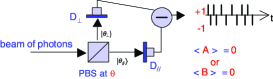
Figure 1: Detection scheme based on balanced homodyne detection for measuring operators $A_{1}$ and $B_{2}$.

In the Stapp’s approach Stapp (99) for a two photon entangled state $|\psi^{\pm}\rangle$=$\frac{1}{\sqrt{2}}\left(|H_{1}V_{2}\rangle\pm|V_{1}H_{2}\rangle\right)$, the two entangled photons are sent to two spatially separated measuring devices A and B. Device A is an analyzer for projecting the linear polarization of the incoming photon. When the analyzer A is oriented along the polarization angle $\theta_{1}$, the polarization state of the incoming photon is projected onto the state,

$$|\theta_{1}\rangle = \cos\theta_{1}|H_{1}\rangle+\sin\theta_{1}|V_{1}\rangle$$ (1)

where H and V are horizontal and vertical axes. The corresponding orthogonal polarization state is given by

$$|\theta_{1}^{\perp}\rangle = -\sin\theta_{1}|H_{1}\rangle+\cos\theta_{1}|V_{1}\rangle$$ (2)

The operator associated with analyzer A can be represented as $A_{1}$, which is defined as Stapp (99)

$$A_{1} = 2|\theta_{1}\rangle\langle\theta_{1}|-\left(|\theta_{1}\rangle\langle\theta_{1}|+|\theta_{1}^{\perp}\rangle\langle\theta_{1}^{\perp}|\right)\,.$$ (3)

The operator $A_{1}$ has eigenvalues of $\pm 1$, such that,

$$A_{1}|\theta_{1}\rangle = 1\,|\theta_{1}\rangle$$

$$A_{1}|\theta_{1}^{\perp}\rangle = -1\,|\theta_{1}^{\perp}\rangle\,$$ (4)

depending on whether the photon is transmitted ($\parallel$) or rejected ($\perp$ ) by the analyzer. Similarly, the analyzer B oriented along polarization angle $\theta_{2}$ can be defined as operator $B_{2}$. One should note that the operator $A_{1}(B_{2})$ with eigenvalues of $\pm 1$ could be measured by using the detection scheme as shown in Fig. 1. Two detectors are placed at the two output ports of a cube polarization beam splitter (PBS). Their output currents are subtracted from each other. The arrangement of this detection scheme can be used for measuring operator $A_{1}$ of Eq.(3), that is the subtraction between the projection of the transmitted signal $|\theta_{1}\rangle_{\parallel}\langle\theta_{1}|$ and the projection of the reflected signal $|\theta_{1}\rangle_{\perp}\langle\theta_{1}|$. Let’s consider a beam of photons incidents on the PBS, if one photon goes through the PBS, it will produce non-zero signal at detector $D_{\parallel}$ and zero signals at detector $D_{\perp}$. Then, the subtraction yields positive signal as of $D_{\parallel}-D_{\perp}\geq 0$. If a photon is reflected from the PBS, it will go to the detector $D_{\perp}$ and produce non-zero signal at detector $D_{\perp}$ and zero signals at detector $D_{\parallel}$. Then, the subtraction yields negative signal as of $D_{\parallel}-D_{\perp}\geq 0$. For a certain amount of time, the subtraction records the random positive and negative spikes corresponding to the eigenvalues of +1 and -1 of operator $A_{1}$, respectively, as shown in the inset of Fig. 1. The incoming photons are in the superposition of $|\theta_{1}\rangle_{\parallel}$ and $\theta_{1}\rangle_{\perp}$. Hence, as the time elapses, the detection scheme A records a series of discrete random values, +1 and -1. Then, for a state with equal probabilities of $\parallel$ and $\perp$ photons, the mean value of $A_{1}$ is zero, that is $\langle A_{1}\rangle$ = 0. Similarly, we can apply the same detection scheme for measuring operator $B_{2}$. We will obtain $\langle B_{2}\rangle=0$. It is very important to show that the detection scheme exhibits wave-particle duality principle. The wave character of the operator $A_{1}(B_{2})$ is recognized as interference of the outcomes of $A_{1}(B_{2})$ due to the linear superposition of the projected states $|\theta\rangle_{\parallel}\langle\theta|$ and $|\theta\rangle_{\perp}\langle\theta|$. The particle character of the operator $A_{1}(B_{2})$ is the discreteness of random values of +1 and -1. The product of the operators $A_{1}$ and $B_{2}$ or the multiplication of their output signals will produce correlation functions, as given by,

$$C_{q}(\theta_{1},\theta_{2})=\langle\psi^{\pm}|A_{1}B_{2}|\psi^{\pm}\rangle=-\cos 2(\theta_{1}\pm\theta_{2})\,.$$ (5)

Eq.5 is usually referred to as the expectation value for the product of operators $A_{1}$ and $B_{2}$. For the other two Bell states, $|\varphi^{\pm}\rangle=\frac{1}{\sqrt{2}}\left(|H_{1}H_{2}\rangle\pm|V_{1}V_{2}\rangle\right)$, the correlation functions are given by,

$$C_{q}(\theta_{1},\theta_{2})=\langle\varphi^{\pm}|A_{1}B_{2}|\varphi^{\pm}\rangle=\cos 2(\theta_{1}\mp\theta_{2})\,.$$ (6)

.

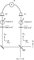
Figure 2: Experimental setup for demonstrating Stapp’s formulation of nonlocality based on coherent fields.

The proof-of principle experimental setup is shown in Fig. 2. The coherent light source is a HeNe laser operated at 632nm. A vertically polarized beam is a coherent light field $\bf V_{S}$ with frequency shifted at 110 MHz. A horizontally polarized beam is a random phase-modulated light field $\bf H_{N}$ induced by an variable acoustic optics modulator at around 110 MHz, which is externally added and modulated by a random noise generator. These two light fields are then combined through a beam splitter. The beam 1 from the output port 1 of the beam splitter contains a superposition of vertically polarized coherent field and horizontally polarized noise field. Similarly, for the beam 2 from the output port 2 of the beam splitter. A quarter wave plate at $45^{o}$ as part of measuring device is inserted at beams 1 and 2 to transform the linearly polarized states to circularly polarized states. By using a quarter wave plate transformation matric, the fields amplitudes $\bf V_{S1}$, $\bf H_{N1}$, $\bf V_{S2}$ and $\bf H_{N2}$ are transformed as,

$$\bf V_{S1} \rightarrow -i\hat{\bf H}_{S1}+\hat{\bf V}_{S1}$$

$$\bf H_{N1} \rightarrow \hat{\bf H}_{N1}-i\hat{\bf V}_{N1}$$

$$\bf V_{S2} \rightarrow -i\hat{\bf H}_{S2}+\hat{\bf V}_{S2}$$

$$\bf H_{N2} \rightarrow -\hat{\bf H}_{N2}+i\hat{\bf V}_{N2}\,.$$

For simplicity we use unit vector notation and drop the amplitude of fields notation. Now, analyzer A in beam 1 will experience homogeneous superposition of left circularly polarized coherent field and right circularly polarized coherent noise field. Similarly, for analyzer B in beam 2. Analyzer $A(B)$ is placed before the detector 1(2) to project out the phase angle $\theta_{1}$($\theta_{2}$) as,

$$\hat{e}_{1} = \cos\theta_{1}\,\hat{H}+\sin\theta_{1}\,\hat{V}$$

$$\hat{e}_{2} = \cos\theta_{2}\,\hat{H}+\sin\theta_{2}\,\hat{V}.$$ (8)

The superposed field in beam 1 after the $\lambda/4$ plate and the analyzer is,

$$\textbf{E}_{1}(t) = [(\hat{\textbf{H}}_{N1}-i\hat{\textbf{V}}_{N1})e^{-i(\omega+\Omega)t-i\phi}$$ (9)

$$+ (-i\hat{\textbf{H}}_{S1}+\hat{\textbf{V}}_{S1})e^{-i(\omega+\Omega)t}]\cdot\hat{\textbf{e}}_{1}$$

$$= (\cos\theta_{1}-i\sin\theta_{1})e^{-i(\omega+\Omega)t-i\phi}$$

$$+ (-i\cos\theta_{1}+\sin\theta_{1})e^{-i(\omega+\Omega)t}$$

and similarly for the superposed field in beam 2,

$$\textbf{E}_{2}(t) = [(-\hat{\textbf{H}}_{N2}+i\hat{\textbf{V}}_{N2})e^{-i(\omega+\Omega)t-i\phi}$$ (10)

$$+ (-i\hat{\textbf{H}}_{S2}+\hat{\textbf{V}}_{S2})e^{-i(\omega+\Omega)t}]\cdot\hat{\textbf{e}}_{2}$$

$$= (-\cos\theta_{2}+i\sin\theta_{2})e^{-i(\omega+\Omega)t-i\phi}$$

$$+ (-i\cos\theta_{2}+\sin\theta_{2})e^{-i(\omega+\Omega)t}$$

where $\omega$ and $\Omega$ are optical and modulated frequencies, and $\phi$ is a random phase of the noise field. Instead of using the detection scheme as shown in Fig. 1, a detector (Hamamatsu S1223-01 with detection bandwidth of 20 MHz) with a DC block will provide the similar result except the 3 dB gain in the balanced detection.

Thus, the interference signals obtained in detectors 1 and 2 can be written as,

$$D_{1}(\phi) = -ie^{i(2\theta_{1}+\phi)}+c.c$$

$$= \sin(2\theta_{1}+\phi)$$

$$D_{2}(\phi) = ie^{i(2\theta_{2}+\phi)}+c.c$$ (11)

$$= -\sin(2\theta_{2}+\phi).$$

The interference signals of Eq. 11 for detectors 1 and 2 are the measurements of operators $A_{1}$ and $B_{2}$, respectively. The interference signal in detector 2 is anti-correlated to detector 1 because of the $\pi$ phase shift of the beam splitter. The interference signals contain information of the projection angles of the analyzers, which are protected by the random noise phases, $\phi$. The average of the interference signals is zero, that is, $\langle A_{1}\rangle$ = 0 and $\langle B_{2}\rangle$ = 0. To further discuss the significant of measuring the operator $A_{1}$, the interference signals obtained in detector 1 can be rewritten as,

$$A_{1}(\phi) = \cos(2\theta_{1})\sin(\phi)+\sin(2\theta_{1})\cos(\phi)$$ (12)

Eq. 12 is identical in structure with operator $A_{1}$ as in Eq. 3, that is

$$A_{1} = \cos 2\theta_{1}(|V_{1}\rangle\langle V_{1}|-|H_{1}\rangle\langle H_{1}|)$$

$$+ \sin 2\theta_{1}(|V_{1}\rangle\langle H_{1}|+|H_{1}\rangle\langle V_{1}|).$$

Note that the unit polarization projectors $(|V_{1}\rangle\langle V_{1}|-|H_{1}\rangle\langle H_{1}|)$ and $(|V_{1}\rangle\langle H_{1}|+|H_{1}\rangle\langle V_{1}|)$ in Eq. LABEL:eq:noise17 can be interpreted by in-phase and out-of-phase or out-of-phase and in-phase components of the noise field because of random noise phase, $\phi$. The interference signals in detectors 1 and 2 are then multiplied to obtain the anti-correlated multiplication signal,

$$A_{1}\times B_{2} = -\sin(2\theta_{1}+\phi)\sin(2\theta_{2}+\phi)$$

$$= -\cos(2(\theta_{1}-\theta_{2}))-\cos(2(\theta_{1}+\theta_{2}+\phi))$$

Then, the mean value of this multiplied signal is measured. We obtain the correlation function $C(\theta_{1},\theta_{2})$,

$$\overline{A_{1}\times B_{2}} \propto C(\theta_{1},\theta_{2})\propto-\cos(2(\theta_{1}-\theta_{2}))$$ (15)

where the random noise phases term in Eq. LABEL:eq:noise18 is averaging to zero. We have projected out the polarization-entangled state $|\psi^{-}\rangle=\frac{1}{\sqrt{2}}[|H_{1}V_{2}\rangle-|V_{1}H_{2}\rangle]$. We normalized the correlation function $C(\theta_{1},\theta_{2})$ with its maximum obtainable value that is $\theta_{1}=\theta_{2}$. Thus, for the setting of the analyzers at $\theta_{1}=\theta_{2}$, the normalized correlation function $C^{N}(\theta_{1},\theta_{2})=-1$ shows that the two beams are anti-correlated.

For other Bell’s state preparation, such as, $|\psi^{+}\rangle=\frac{1}{\sqrt{2}}[|H_{1}V_{2}\rangle+|V_{1}H_{2}\rangle]$, the $\lambda/4$ wave plate at beam 2 is rotated at -$45^{\circ}$, then the beat signal $B_{2}$ of Eq. 11 is given by

$$B_{2}(\phi)\propto-\sin(2\theta_{2}-\phi)\,.$$ (16)

Hence, the correlation function of Eq. 15 is

$$C(\theta_{1},\theta_{2})\propto-\cos 2(\theta_{1}+\theta_{2})$$ (17)

corresponding to the projected polarization-entangled state $|\psi^{+}\rangle$.

As for the state $|\varphi^{+}\rangle=\frac{1}{\sqrt{2}}[|H_{1}H_{2}\rangle+|V_{1}V_{2}\rangle]$, a $\lambda/2$ plate in beam 2 is inserted, then the minus sign of beat signal $B_{2}$ of Eq. 11 is changed to positive sign. The correlation function of Eq. 15 is $\propto$ $\cos 2(\theta_{1}-\theta_{2})$. Thus, the $C(\theta_{1},\theta_{2})=+1$ for $\theta_{1}=\theta_{2}$, then the projected polarization-entangled state is perfect correlated that is $|\varphi^{+}\rangle$.

Similarly, with the $\lambda/2$ wave plate at beam 2 and the $\lambda/4$ wave plate at beam 2 rotated at -$45^{\circ}$, the beat signal $B_{2}$ of Eq. 11 is $=\sin(2\theta_{2}-\phi)$. Thus, the correlation function of Eq. 15 is $\propto$ $\cos 2(\theta_{1}+\theta_{2})$ corresponding to the projected polarization-entangled state $|\varphi^{-}\rangle=\frac{1}{\sqrt{2}}[|H_{1}H_{2}\rangle-|V_{1}V_{2}\rangle$. The scheme is perfect for quantum communication processing because the four Bell states are prepared by just changing the phases in beam 2. For practical quantum communication, Alice can keep the beam 2 and sent out the beam 1 to Bob. Since Alice can change the phases of beam 2 locally, her acts will change the non-local correlation function with Bob.

As for an illustration of our experimental observation for the correlation function $C(\theta_{1},\theta_{2})=-\cos 2(\theta_{1}-\theta_{2})$ of the state $|\psi^{-}\rangle$, we take a single shot of the anti-correlated beat signal at detectors 1 and 2 for $\theta_{1}=\theta_{2}$ as shown in Fig. 3a and b respectively. One may notice that the mean value of beat signal $\langle A_{1}\rangle$ and $\langle B_{2}\rangle$ are zero as predicted. The multiplied beat signal is shown in Fig. 3c which has the maximum obtainable mean value. Also shown in Fig. 3d is the multiplied beat signal for the case $\theta_{1}=0$ and $\theta_{2}=45$, where its mean value approximately zero as predicted by $C(\theta_{1},\theta_{2})$.

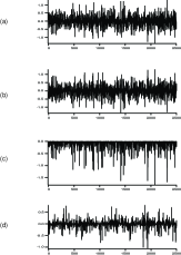
Figure 3: (a)A single shot of the beat signal at detector 1 and (b) detector 2; (c) the multiplied beat signal for $\theta_{1}=\theta_{2}$ and (d) for $\theta_{1}=0,\theta_{2}=45^{\circ}$.

To further verify the nonlocality between these two spatially separated beams, the correlation functions between two distant observers ($A_{1}$ and $B_{2})$ are measured for the violation of Bell Inequality Bell (1978), which is given by Peres (1993),

$$|C^{N}(a,b)-C^{N}(a,c)|\leq 1+C^{N}(b,c)$$

or,

$$F(a,b,c) = |C^{N}(a,b)-C^{N}(a,c)|-1-C^{N}(b,c)|\leq 0.$$

where $\bf a$, $\bf b$ and $\bf c$ are projection angles of the analyzers A and B. For the entangled state, $|\psi^{-}\rangle=\frac{1}{\sqrt{2}}[|H_{1}V_{2}\rangle-|V_{1}H_{2}\rangle]$, the correlation function $-\cos(2(\theta_{1}-\theta_{2}))$ is used.

Maximum violation of Bell inequality of Eq. LABEL:eq:noise20 can be demonstrated as analyzer A chooses polarization angles along the axes a=$0^{o}$ and b=$30^{o}$ and analyzer B chooses along the axes b=$30^{o}$ and c=$60^{o}$. First, we fixed the $a=\theta_{1}=0$, then varied $c=\theta_{2}$ from $0^{o}$ to $90^{o}$ to obtain the correlation function $C^{N}(a=0^{o},c=\theta_{2})$ as shown in Fig. 4a. Second, we fixed $\theta_{1}=30^{o}$ and varied $\theta_{2}$ from $0^{o}$ to $90^{o}$. The correlation function $C^{N}(b=30^{o},c=\theta_{2})$ is measured and shown in Fig. 4b. By using the above measurements, we plot $F(a,b,c)=|C^{N}(a=0^{o},b=30^{o})-C^{N}(a=0^{o},c)|-1-C^{N}(b=30^{o},c)$ as a function of $c=\theta_{2}$ as shown in Fig. 4c. The solid lines in the figures are theoretical predictions by using $C^{N}(\theta_{1},\theta_{2})=-\cos 2(\theta_{1}-\theta_{2})$. The experimental results show that the maximum violation value is +0.5 occurs at the $c=\theta_{2}=60^{o}$, $F(a,b,c)\not\leq 0$.

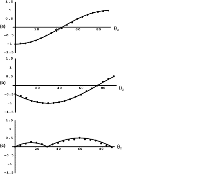
Figure 4: (a) The measurement of correlation functions ,$C^{N}(a=0^{o},c=\theta_{2})$ and (b)$C^{N}(b=30^{o}c=\theta_{2})$; (c) the plot of $F(a,b,c)=|C^{N}(a=0^{o},b=30^{o})-C^{N}(a=0^{o},c)|-1-C^{N}(b=30^{o},c)$ showing $F(a,b,c)\not\leq 0$, maximum violation occurs at $c=\theta_{2}=60^{o}$.

The experiment has demonstrated nonlocality of two distant observers based on superposition of one coherent light field and one coherent noise field. This newly developed scheme can be implemented together with the time-bin method for entanglement distributions and key distributions, such as Ekert’s protocol. For the prepared state $|\psi^{-}\rangle=\frac{1}{\sqrt{(}2)}[|H_{1}V_{2}\rangle-|V_{1}H_{2}\rangle]$, the anti-correlation function is given by $-\cos(2(\theta_{1}-\theta_{2}))$, where $\theta_{1}=\theta_{2}$ for maximum anti-correlation. When the beat signal at detector 1 has a positive (negative) signal, the beat signal in detector 2 has a negative (positive) signal. The random positive and negative beat signals can be encoded for qubit implementation. The positive signal is encoded to qubit ”1” and the negative signal is encoded to qubit ”0”. This encoding process can be conducted by using a comparator after the detectors 1 and 2. If two coherent states, $|\alpha\rangle=|\alpha|e^{-i\phi_{\alpha}}$ and $|\beta\rangle=|\beta|e^{-i\phi_{\beta}}$, with low mean photon numbers are used, their quantum phase fluctuations, $\phi_{\alpha}$, $\phi_{\beta}$ will play an essential role of randomness in this newly developed scheme.

In conclusion, we have shown that the random and anti-correlated beat signals at two spatially separated beams created by the superposition of the coherent light field and the noise field can exhibit the nonlocality and the duality properties of operators $A_{1}$ and $B_{2}$. The scheme is perfect for long distance entanglement distribution and key distribution. The experimental observation has also implied that phase fluctuation and beam splitter transformation are the origin creation of entanglement and nonlocality for two coherent light fields.