The Distribution of the Domination Number of Class Cover Catch Digraphs for Non-uniform One-dimensional Data

Abstract

For two or more classes of points in $\mathbb{R}^{d}$ with $d\geq 1$, the class cover catch digraphs (CCCDs) can be constructed using the relative positions of the points from one class with respect to the points from the other class. The CCCDs were introduced by Priebe et al., (2001) who investigated the case of two classes, $\mathcal{X}$ and $\mathcal{Y}$. They calculated the exact (finite sample) distribution of the domination number of the CCCDs based on $\mathcal{X}$ points relative to $\mathcal{Y}$ points both of which were uniformly distributed on a bounded interval. We investigate the distribution of the domination number of the CCCDs based on data from non-uniform $\mathcal{X}$ points on an interval with end points from $\mathcal{Y}$. Then we extend these calculations for multiple $\mathcal{Y}$ points on bounded intervals.

Keywords: Class Cover Catch Digraph; Domination number; Non-uniform Distribution; Proximity Map; Random digraph

1 Introduction

In 2001, a new classification method was developed which was based on the relative positions of the data points from various classes; Priebe et al., (2001) introduced the class cover catch digraphs (CCCDs) in $\mathbb{R}$ and gave the exact distribution of the domination number of the CCCDs for two classes, $\mathcal{X}$ and $\mathcal{Y}$, with uniform distribution on a bounded interval in $\mathbb{R}$. DeVinney and Wierman, (2003) proved a SLLN result for the one-dimensional class cover problem. DeVinney et al., (2002), Marchette and Priebe, (2003), Priebe et al., 2003a , and Priebe et al., 2003b extended the CCCDs to higher dimensions and demonstrated that CCCDs are a competitive alternative to the existing methods in classification. The classification method based on CCCDs involves data reduction (condensing) by using approximate — rather than exact — minimum dominating sets as prototype sets, since finding the exact minimum dominating set for CCCDs is an NP-hard problem in general. However for finding a dominating set of CCCDs on the real line, a simple linear time algorithm is available (Priebe et al., (2001)). But unfortunately, the exact and the asymptotic distributions of the domination number of the CCCDs are not analytically tractable in multiple dimensions.

To address the latter issue of intractability of the distribution of the domination number in multiple dimensions, Ceyhan and Priebe, (2003, 2005) introduced the central similarity proximity maps and $r$-factor proportional-edge proximity maps and the associated random proximity catch digraphs. Proximity catch digraphs are a generalization of the CCCDs. The asymptotic distribution of the domination number of the latter is calculated and then used in testing spatial patterns between two or more classes. See Ceyhan and Priebe, (2005) for more detail.

In this article, we generalize the original result of Priebe et al., (2001) to the case of non-uniform $\mathcal{X}$ points with support being the interval with end points from $\mathcal{Y}$, and then to multiple $\mathcal{Y}$ points in a bounded interval $(c,d)\subset\mathbb{R}$ with $c<d$. These generalizations will also serve as the bases for extension of the results for the uniform and non-uniform data in higher dimensions.

2 Data-random Class Cover Catch Digraphs

Let $(\Omega,\mathcal{M})$ be a measurable space and $\mathcal{X}_{n}=\{X_{1},\ldots,X_{n}\}$ and $\mathcal{Y}_{m}=\{Y_{1},\ldots,Y_{m}\}$ be two sets of $\Omega$-valued random variables from classes $\mathcal{X}$ and $\mathcal{Y}$, respectively, with joint probability distribution $F_{X,Y}$. Let $d(\cdot,\cdot):\Omega\times\Omega\rightarrow[0,\infty)$ be any distance function. The class cover problem for a target class, say $\mathcal{X}$, refers to finding a collection of neighborhoods, $N_{i}$ around $X_{i}$ such that (i) $\mathcal{X}_{n}\subseteq\bigl{(}\cup_{i}N_{i}\bigr{)}$ and (ii) $\mathcal{Y}_{m}\cap\bigl{(}\cup_{i}N_{i}\bigr{)}=\emptyset$. A collection of neighborhoods satisfying both conditions is called a class cover. A cover satisfying condition (i) is a proper cover of class $\mathcal{X}$ while a cover satisfying condition (ii) is a pure cover relative to class $\mathcal{Y}$. This article is on the minimum cardinality class covers; that is, class covers satisfying both (i) and (ii) with the smallest number of neighborhoods. See Priebe et al., (2001).

Consider the map $N:\Omega\rightarrow 2^{\Omega}$ where $2^{\Omega}$ represents the power set of $\Omega$. Then given $\mathcal{Y}_{m}\subseteq\Omega$, the proximity map $N_{\mathcal{Y}}(\cdot):\Omega\rightarrow 2^{\Omega}$ associates with each point $x\in\Omega$ a proximity region $N_{\mathcal{Y}}(x)\subseteq\Omega$. For $B\subseteq\Omega$, the $\Gamma_{1}$-region is the image of the map $\Gamma_{1}(\cdot,N_{\mathcal{Y}}):2^{\Omega}\rightarrow 2^{\Omega}$ that associates the region $\Gamma_{1}(B,N_{\mathcal{Y}}):=\{z\in\Omega:B\subseteq N_{\mathcal{Y}}(z)\}$ with the set $B$. For a point $x\in\Omega$, we denote $\Gamma_{1}(\{x\},N_{\mathcal{Y}})$ as $\Gamma_{1}(x,N_{\mathcal{Y}})$. Notice that while the proximity regions are defined for one point, $\Gamma_{1}$-regions are defined for sets of points.

The data-random CCCD has the vertex set $\mathcal{V}=\mathcal{X}_{n}$ and arc set $\mathcal{A}$ defined by $(X_{i},X_{j})\in\mathcal{A}\iff X_{j}\in N_{\mathcal{Y}}(X_{i})$. In particular, we use $N_{\mathcal{Y}}(X_{i})=B(X_{i},r_{i})$, the open ball around $X_{i}$ with radius $r_{i}:=\min_{Y\in\mathcal{Y}_{m}}d(X_{i},Y)$, as the proximity map as in Priebe et al., (2001). We call such a digraph a $\mathscr{D}_{n,m}$-digraph. A $\mathscr{D}_{n,m}$-digraph is a pseudo digraph according some authors if loops are allowed (see, e.g., Chartrand and Lesniak, (1996)).

A data-random CCCD for $\Omega=\mathbb{R}^{d}$ and $N_{i}=B(X_{i},r_{i})$ is referred to as $\mathscr{C}_{n,m}$-graph in Priebe et al., (2001). We change the notation to emphasize the fact that $\mathscr{D}_{n,m}$ is a digraph. Furthermore, Ceyhan and Priebe, (2003) call the proximity map $N_{i}=B(X_{i},r_{i})$ a spherical proximity map.

The $\mathscr{D}_{n,m}$-digraphs are closely related to the proximity graphs of Jaromczyk and Toussaint, (1992) and might be considered as a special case of covering sets of Tuza, (1994) and intersection digraphs of Sen et al., (1989). Our data-random proximity digraph is a vertex-random proximity digraph and not a standard one (see e.g., Janson et al., (2000)). The randomness of a $\mathscr{D}_{n,m}$-digraph lies in the fact that the vertices are random with the joint distribution $F_{X,Y}$, but arcs $(X_{i},X_{j})$ are deterministic functions of the random variable $X_{j}$ and the random set $N_{i}$.

3 Domination Number of Random $\mathscr{D}_{n,m}$-digraphs

In a digraph $D=(\mathcal{V},\mathcal{A})$ of order $|\mathcal{V}|=n$, a vertex $v$ dominates itself and all vertices of the form $\{u:\,(v,u)\in\mathcal{A}\}$. A dominating set, $S_{D}$, for the digraph $D$ is a subset of $\mathcal{V}$ such that each vertex $v\in\mathcal{V}$ is dominated by a vertex in $S_{D}$. A minimum dominating set, $S^{*}_{D}$, is a dominating set of minimum cardinality; and the domination number, denoted $\gamma(D)$, is defined as $\gamma(D):=|S^{*}_{D}|$, where $|\cdot|$ is the set cardinality functional (West, (2001)). If a minimum dominating set consists of only one vertex, we call that vertex a dominating vertex. The vertex set $\mathcal{V}$ itself is always a dominating set, so $\gamma(D)\leq n$.

Let $\mathcal{F}\left(\mathbb{R}^{d}\right):=\{F_{X,Y}\text{ on }\mathbb{R}^{d}\text{ with }P(X=Y)=0\}$. As in Priebe et al., (2001), in this article, we consider $\mathscr{D}_{n,m}$-digraphs for which $\mathcal{X}_{n}$ and $\mathcal{Y}_{m}$ are random samples from $F_{X}$ and $F_{Y}$, respectively, and the joint distribution of $X,Y$ is $F_{X,Y}\in\mathcal{F}\left(\mathbb{R}^{d}\right)$. We call such digraphs as $\mathcal{F}\left(\mathbb{R}^{d}\right)$-random $\mathscr{D}_{n,m}$-digraphs and focus on the random variable $\gamma(D)$. To make the dependence on sample sizes explicit, we use $\gamma(D_{n,m})$ instead of $\gamma(D)$. It is trivial to see that $1\leq\gamma(D_{n,m})\leq n$, and $\gamma(D_{n,m})<n$ for nontrivial digraphs.

4 The Distribution of the Domination Number of $\mathcal{F}(\mathbb{R})$-random $\mathscr{D}_{n,m}$-digraphs

In $\mathbb{R}$, the data-random CCCD is a special case of interval catch digraphs (see, e.g., Sen et al., (1989) and Prisner, (1994)). Let $\mathcal{X}_{n}$ and $\mathcal{Y}_{m}$ be two samples from $\mathcal{F}(\mathbb{R})$ and $Y_{(j)}$ be the $j^{th}$ order statistic of $\mathcal{Y}_{m}$ for $j=1,2,\ldots,m$. Then $Y_{(j)}$ partition $\mathbb{R}$ into $(m+1)$ intervals. Let

$$-\infty=:Y_{(0)}<Y_{(1)}<\ldots<Y_{(m)}<Y_{(m+1)}:=\infty,$$

and $\mathcal{I}_{j}:=\left(Y_{(j-1)},Y_{(j)}\right)$, $\mathcal{X}^{j}:=\mathcal{X}_{n}\cap\mathcal{I}_{j}$, and $\mathcal{Y}^{j}:=\{Y_{(j-1)},Y_{(j)}\}$ for $j=1,2,\ldots,(m+1)$. This yields a disconnected digraph with subdigraphs $D^{j}$ for $j=1,2,\ldots,(m+1)$, each of which might be null or itself disconnected. Let $\gamma(D^{j})$ denote the the cardinality of the minimum dominating set for the component of the random $\mathscr{D}_{n,m}$-digraph induced by the pair $\mathcal{X}^{j}$ and $\mathcal{Y}^{j}$, $n_{j}:=|\mathcal{X}^{j}|$, and $F_{j}$ be the density $F_{X}$ restricted to $\mathcal{I}_{j}$. Then $\gamma(D_{n,m})=\sum_{j=1}^{m+1}\gamma(D^{j})$. We study the simpler random variable $\gamma(D^{j})$ first. The following lemma follows trivially (see Priebe et al., (2001)).

Lemma 4.1.

For $j\in\{1,(m+1)\}$, $\gamma(D^{j})=\mathbf{I}(n_{j}>0)$ where $\mathbf{I}(\cdot)$ is the indicator function.

For $j=2,\ldots,m$ and $n_{j}>0$, we prove that $\gamma(D^{j})\in\{1,2\}$ with the distribution dependent probabilities $1-p_{n_{j}}(F_{j}),p_{n_{j}}(F_{j})$, respectively, where $p_{n_{j}}(F_{j})=P(\gamma(D^{j})=2)$. A quick investigation shows that $\gamma(D^{j})=2$ iff $\mathcal{X}^{j}\cap\left(\frac{\max\,(\mathcal{X}^{j})+Y_{(j-1)}}{2},\frac{\min(\mathcal{X}^{j})+Y_{(j)}}{2}\right)=\emptyset$; that is, $\mathcal{X}^{j}\subset B(x,r(x))$ iff $x\in\left(\frac{\max\,(\mathcal{X}^{j})+Y_{(j-1)}}{2},\frac{\min(\mathcal{X}^{j})+Y_{(j)}}{2}\right)$ where $r(x)=\min(x-Y_{(j-1)},Y_{(j)}-x)$. Hence $\Gamma_{1}(\mathcal{X}^{j},N_{\mathcal{Y}})=\left(\frac{\max\,(\mathcal{X}^{j})+Y_{(j-1)}}{2},\frac{\min(\mathcal{X}^{j})+Y_{(j)}}{2}\right)\subseteq\mathcal{I}_{j}$. By definition, if $\mathcal{X}^{j}\cap\Gamma_{1}(\mathcal{X}^{j},N_{\mathcal{Y}})\not=\emptyset$, then $\gamma(D^{j})=1$; hence the name $\Gamma_{1}$-region and the notation $\Gamma_{1}(\cdot,N_{\mathcal{Y}})$.

Theorem 4.2.

For $j=2,\ldots,m$, $\gamma(D^{j})\sim 1+\operatorname{Bernoulli}(p_{n_{j}}(F_{j}))$ for $n_{j}>0$.

Proof: See Priebe et al., (2001) for the proof. $\blacksquare$

The probability $P(\gamma(D^{j})=2)=P(\mathcal{X}^{j}\cap\Gamma_{1}(\mathcal{X}^{j},N_{\mathcal{Y}})=\emptyset)$ depends on the conditional distribution $F_{X|Y}$ and the interval $\Gamma_{1}(\mathcal{X}^{j},N_{\mathcal{Y}})$, which, if known, will make possible the calculation of $p_{n_{j}}(F_{j})$. As an immediate result of Lemma 4.1 and Theorem 4.2, we have the following upper bound for $\gamma(D_{n,m})$.

Theorem 4.3.

Let $D_{n,m}$ be an $\mathcal{F}(\mathbb{R})$-random $\mathscr{D}_{n,m}$-digraph with $n>0,\,m>0$ and $k_{1}$ and $k_{2}$ be two natural numbers defined as $k_{1}:=\sum_{j=2}^{m}\mathbf{I}(|\mathcal{X}_{n}\cap\mathcal{I}_{j}|>1)$ and $k_{2}:=\sum_{j=2}^{m}\mathbf{I}(|\mathcal{X}_{n}\cap\mathcal{I}_{j}|=1)+\sum_{j\in\{1,(m+1)\}}\mathbf{I}(\mathcal{X}_{n}\cap\mathcal{I}_{j}\not=\emptyset)$. Then $1\leq\gamma(D_{n,m})\leq 2\,k_{1}+k_{2}\leq\min(n,2\,m)$.

In the special case of fixed $\mathcal{Y}_{2}=\{\mathsf{y}_{1},\mathsf{y}_{2}\}$ and $\mathcal{X}_{n}$ a random sample from $\mathcal{U}(\mathsf{y}_{1},\mathsf{y}_{2})$, the uniform distribution on $(\mathsf{y}_{1},\mathsf{y}_{2})$, we have a $\mathscr{D}_{n,2}$-digraph for which $F_{X}=\mathcal{U}(\mathsf{y}_{1},\mathsf{y}_{2})$ and $F_{Y}$ is a degenerate distribution. We call such digraphs as $\mathcal{U}(\mathsf{y}_{1},\mathsf{y}_{2})$-random $\mathscr{D}_{n,2}$-digraphs and provide an exact result on the distribution of their domination number in the next section.

4.1 The Exact Distribution of the Domination Number of $\mathcal{U}(\mathsf{y}_{1},\mathsf{y}_{2})$-random $\mathscr{D}_{n,2}$-digraphs

Suppose $\mathcal{Y}_{2}=\{\mathsf{y}_{1},\mathsf{y}_{2}\}\subset\mathbb{R}$ with $-\infty<\mathsf{y}_{1}<\mathsf{y}_{2}<\infty$ and $\mathcal{X}_{n}=\{X_{1},\ldots,X_{n}\}$ a set of iid random variables from $\mathcal{U}(\mathsf{y}_{1},\mathsf{y}_{2})$. Any $\mathcal{U}(\mathsf{y}_{1},\mathsf{y}_{2})$ random variable can be transformed into a $\mathcal{U}(0,1)$ random variable by $\phi(x)=(x-\mathsf{y}_{1})/(\mathsf{y}_{2}-\mathsf{y}_{1})$, which maps intervals $(t_{1},t_{2})\subseteq(\mathsf{y}_{1},\mathsf{y}_{2})$ to intervals $\bigl{(}\phi(t_{1}),\phi(t_{2})\bigr{)}\subseteq(0,1)$. So, without loss of generality, we can assume $\mathcal{X}_{n}=\{X_{1},\ldots,X_{n}\}$ is a set of iid random variables from the $\mathcal{U}(0,1)$ distribution. That is, the distribution of $\gamma(D_{n,2})$ does not depend on the support interval $(\mathsf{y}_{1},\mathsf{y}_{2})$. Recall that $\gamma(D_{n,2})=2$ iff $\mathcal{X}_{n}\cap\Gamma_{1}(\mathcal{X}_{n},N_{\mathcal{Y}})=\emptyset$, then $P(\gamma(D_{n,2})=2)=4/9-(16/9)\,4^{-n}$. For more detail, see (Priebe et al., (2001)). Hence, for $\mathcal{U}(\mathsf{y}_{1},\mathsf{y}_{2})$ data, we have

$$\gamma(D_{n,2})=\left\{\begin{array}[]{ll}1&\text{w.p. $5/9+(16/9)\,4^{-n},$}\\ 2&\text{w.p. $4/9-(16/9)\,4^{-n},$}\end{array}\text{~{}~{}for all $n\geq 1$},\right.$$ (1)

where w.p. stands for “with probability”. Then the asymptotic distribution of $\gamma(D_{n,2})$ for $\mathcal{U}(\mathsf{y}_{1},\mathsf{y}_{2})$ data is given by

$$\lim_{n\rightarrow\infty}\gamma(D_{n,2})=\left\{\begin{array}[]{ll}1&\text{w.p. $5/9$,}\\ 2&\text{w.p. $4/9$.}\end{array}\right.$$ (2)

For $m>2$, Priebe et al., (2001) computed the exact distribution of $\gamma(D_{n,m})$. However, independence of the distribution of the domination number from the support interval does not hold in general; that is, for $X_{i}\stackrel{{\scriptstyle iid}}{{\sim}}F$ with support $\mathcal{S}(F)\subseteq(\mathsf{y}_{1},\mathsf{y}_{2})$, the exact and asymptotic distribution of $\gamma(D_{n,2})$ will depend on $F$ and $\mathcal{Y}_{2}$.

4.2 The Distribution of the Domination Number for $\mathcal{F}(\mathbb{R})$-random $\mathscr{D}_{n,2}$-digraphs

For $\mathcal{Y}_{2}=\{\mathsf{y}_{1},\mathsf{y}_{2}\}\subset\mathbb{R}$ with $-\infty<\mathsf{y}_{1}<\mathsf{y}_{2}<\infty$, a quick investigation shows that the $\Gamma_{1}$-region is $\Gamma_{1}(\mathcal{X}_{n},N_{\mathcal{Y}})=\left(\frac{\mathsf{y}_{1}+X_{(n)}}{2},\frac{\mathsf{y}_{2}+X_{(1)}}{2}\right)$. Note that $\mathcal{X}_{n}\cap\Gamma_{1}(\mathcal{X}_{n},N_{\mathcal{Y}})$ is the set of all dominating vertices, which is empty when $\gamma(D_{n,2})>1$. To make the dependence on $F$ explicit and for brevity of notation, we will denote the domination number of the $F\bigl{(}(\mathsf{y}_{1},\mathsf{y}_{2})\bigr{)}$-random $\mathscr{D}_{n,2}$-digraphs as $\gamma_{n}(F)$.

Let $p_{n}(F):=P(\gamma_{n}(F)=2)$ and $p(F):=\lim_{n\rightarrow\infty}P(\gamma_{n}(F)=2)$. Then the exact (finite sample) and asymptotic distributions of $\gamma_{n}(F)$ are $1+\operatorname{Bernoulli}\left(p_{n}(F)\right)$ and $1+\operatorname{Bernoulli}\left(p(F)\right)$, respectively. That is, for finite $n$, we have

$$\gamma_{n}(F)=\left\{\begin{array}[]{ll}1&\text{w.p. $1-p_{n}(F)$}\\ 2&\text{w.p. $p_{n}(F)$}\end{array}\text{for all $n\geq 1$}.\right.$$ (3)

The asymptotic distribution is similar.

With $\mathcal{Y}_{2}=\{0,1\}$, let $F$ be a distribution with support $\mathcal{S}(F)\subseteq(0,1)$ and density $f$ and let $\mathcal{X}_{n}$ be a set of $n$ iid random variables from $F$. Since $\gamma_{n}(F)\in\{1,\,2\}$, to find the distribution of $\gamma_{n}(F)$, it suffices to find $P(\gamma_{n}(F)=1)$ or $P\bigl{(}\gamma_{n}(F)=2\bigr{)}$. For computational convenience, we employ the latter in our calculations.

Then

$$p_{n}(F)=\int_{\mathcal{S}(F)\setminus\Gamma_{1}(\mathcal{X}_{n},N_{\mathcal{Y}})}\left[1-\frac{F((1+x_{1})/2)-F(x_{n}/2)}{F(x_{n})-F(x_{1})}\right]^{n-2}f_{1n}(x_{1},x_{n})dx_{n}dx_{1},$$ (4)

where $f_{1n}(x_{1},x_{n})=n\,(n-1)\,\bigl{[}F(x_{n})-F(x_{1})\bigr{]}^{n-2}\,f(x_{1})\,f(x_{n})\;\mathbf{I}(0<x_{1}<x_{n}<1)$ which is the joint probability density function of $X_{(1)},X_{(n)}$.

If the support $\mathcal{S}(F)=(0,1)$, then the region of integration becomes

$$\Bigl{\{}(x_{1},x_{n})\in(0,1)^{2}:\;(1+x_{1})/2\leq x_{n}\leq 1;\;\;0\leq x_{1}\leq 1/3\text{ or }2\,x_{1}\leq x_{n}\leq 1;\;\;1/3\leq x_{1}\leq 1/2\Bigr{\}}.$$

The integrand in Equation (4) simplifies to

$$H(x_{1},x_{n}):=n\,(n-1)f(x_{1})f(x_{n})\bigl{[}F(x_{n})+F\left(x_{n}/2\right)-\left(F\left((1+x_{1})/2\right)+F(x_{1})\right)\bigr{]}^{n-2}.$$ (5)

Let $\mathcal{X}_{n}$ be a set of iid random variables from a continuous distribution $F$ with $\mathcal{S}(F)\subseteq(0,1)$. The simplest of such distributions is $\mathcal{U}(0,1)$, the uniform distribution on $(0,1)$, which yields the simplest exact distribution for $\gamma_{n}(F)$. If $X\sim F$, then by probability integral transform, $F(X)\sim\mathcal{U}(0,1)$. So for any continuous $F$, we can construct a proximity map depending on $F$ for which the distribution of the domination number for the associated digraph will have the same distribution as that of $\gamma_{n}(\mathcal{U}(0,1))$.

Proposition 4.4.

Let $X_{i}\stackrel{{\scriptstyle iid}}{{\sim}}F$ which is an (absolutely) continuous distribution with support $\mathcal{S}(F)=(0,1)$ and $\mathcal{X}_{n}=\{X_{1},\ldots,X_{n}\}$. Define the proximity map $N_{F}(x):=F^{-1}(N_{\mathcal{Y}}(F(x)))=F^{-1}(B(F(x),r(F(x))))$ where $r(F(x))=\min(F(x),1-F(x))$. Then the domination number of the digraph based on $N_{F}$, $\mathcal{X}_{n}$, and $\mathcal{Y}_{2}=\{0,1\}$, is equal in distribution to $\gamma_{n}(\mathcal{U}(0,1))$.

Proof: Let $U_{i}:=F(X_{i})$ for $i=1,\ldots,n$ and $\mathcal{U}_{n}=\{U_{1},\ldots,U_{n}\}$. Hence, by probability integral transform, $U_{i}\stackrel{{\scriptstyle iid}}{{\sim}}\mathcal{U}(0,1)$. Let $U_{(k)}$ be the $k^{th}$ order statistic of $\mathcal{U}_{n}$ for $k=1,\ldots,n$. Furthermore, such an $F$ preserves order; that is, for $x\leq y$, $F(x)\leq F(y)$. So the image of $N_{F}(x)$ under $F$ is $F(N_{F}(x))=N_{\mathcal{Y}}(F(x))=B(F(x),r(F(x)))$ for (almost) all $x\in(0,1)$. Then $F(N_{F}(X_{i}))=N_{\mathcal{Y}}(F(X_{i}))=N_{\mathcal{Y}}(U_{i})$ for $i=1,\ldots,n$. Since $U_{i}\stackrel{{\scriptstyle iid}}{{\sim}}\mathcal{U}(0,1)$, the distribution of the domination number of the digraph based on $N_{\mathcal{Y}}$, $\mathcal{U}_{n}$ and $\{0,1\}$ is given in Equation (1). Observe that $X_{j}\in N_{F}(X_{i})$ iff $X_{j}\in F^{-1}(B(F(X_{i}),r(F(X_{i}))))$ iff $F(X_{j})\in B(F(X_{i}),r(F(X_{i})))$ iff $U_{j}\in B(U_{i},r(U_{i}))$ for $i,j=1,\ldots,n$. Hence $P(\mathcal{X}_{n}\subset N_{F}(X_{i}))=P(\mathcal{U}_{n}\subset N_{\mathcal{Y}}(U_{i}))$ for all $i=1,\ldots,n$. Therefore, $\mathcal{X}_{n}\cap\Gamma_{1}(\mathcal{X}_{n},N_{F})=\emptyset$ iff $\mathcal{U}_{n}\cap\Gamma_{1}(\mathcal{U}_{n},N_{\mathcal{Y}})=\emptyset$, which implies that the domination number of the digraph based on $N_{F}$, $\mathcal{X}_{n}$, and $\mathcal{Y}_{2}=\{0,1\}$ is 2 with probability $4/9-(16/9)\,4^{-n}$. Hence the desired result follows. $\blacksquare$

For example for $F(x)=x^{2}\,\mathbf{I}(0\leq x\leq 1)+\mathbf{I}(x>1)$,

$$N_{F}(x)=\left\{\begin{array}[]{ll}\left(0,\sqrt{2}\,x\right)&\text{for $x\in\left[0,1/\sqrt{2}\,\right],$}\vspace{.025in}\\ \left(\sqrt{2\,x^{2}-1},1\right)&\text{for $x\in\left(1/\sqrt{2},1\,\right].$}\end{array}\right.$$

There is also a stochastic ordering between $\gamma_{n}(F)$ and $\gamma_{n}(\mathcal{U}(0,1))$ provided that $F$ satisfies some conditions which are given in the following proposition.

Proposition 4.5.

Suppose $\mathcal{X}_{n}=\{X_{1},\ldots,X_{n}\}$ is a random sample from a continuous distribution $F$ with $\mathcal{S}(F)\subseteq(0,1)$ and let $X_{(j)}$ be the $j^{th}$ order statistic of $\mathcal{X}_{n}$ for $j=1,\ldots,n$. If

$$F\bigl{(}X_{(n)}/2\bigr{)}<F\left(X_{(n)}\right)/2\text{ and }F\bigl{(}X_{(1)}\bigr{)}<2\,F\left(\left(1+X_{(1)}\right)/2\right)-1\text{ hold a.s., }$$ (6)

then $\gamma_{n}(F)<^{ST}\gamma_{n}(\mathcal{U}(0,1))$. If $<$’s in expression (6) are replaced with $>$’s, then $\gamma_{n}(F)>^{ST}\gamma_{n}(\mathcal{U}(0,1))$. If $<$’s in expression (6) are replaced with $=$’s, then $\gamma_{n}(F)\stackrel{{\scriptstyle d}}{{=}}\gamma_{n}(\mathcal{U}(0,1))$ where $\stackrel{{\scriptstyle d}}{{=}}$ stands for equality in distribution.

Proof: Let $U_{i}:=F(X_{i})$ for $i=1,\ldots,n$ and $\mathcal{U}_{n}=\{U_{1},\ldots,U_{n}\}$. Then, by probability integral transform, $U_{i}\stackrel{{\scriptstyle iid}}{{\sim}}\mathcal{U}(0,1)$. Let $U_{(j)}$ be the $j^{th}$ order statistic of $\mathcal{U}_{n}$ for $j=1,\ldots,n$. The $\Gamma_{1}$-region for $\mathcal{U}_{n}$ based on $N_{\mathcal{Y}}$ is $\Gamma_{1}(\mathcal{U}_{n},N_{\mathcal{Y}})=\left(U_{(n)}/2,\,\left(1+U_{(1)}\right)/2\right)$; likewise, $\Gamma_{1}(\mathcal{X}_{n},N_{\mathcal{Y}})=\left(X_{(n)}/2,\,\left(1+X_{(1)}\right)/2\right)$. But the conditions in expression (6) imply that $\Gamma_{1}(\mathcal{U}_{n},N_{\mathcal{Y}})\subsetneq F(\Gamma_{1}(\mathcal{X}_{n},N_{\mathcal{Y}}))$. So $\mathcal{U}_{n}\cap F(\Gamma_{1}(\mathcal{X}_{n},N_{\mathcal{Y}}))=\emptyset$ implies that $\mathcal{U}_{n}\cap\Gamma_{1}(\mathcal{U}_{n},N_{\mathcal{Y}})=\emptyset$ and $\mathcal{U}_{n}\cap F(\Gamma_{1}(\mathcal{X}_{n},N_{\mathcal{Y}}))=\emptyset$ iff $\mathcal{X}_{n}\cap\Gamma_{1}(\mathcal{X}_{n},N_{\mathcal{Y}})=\emptyset$. Hence

$$p_{n}(F)=P(\mathcal{X}_{n}\cap\Gamma_{1}(\mathcal{X}_{n},N_{\mathcal{Y}})=\emptyset)<P(\mathcal{U}_{n}\cap\Gamma_{1}(\mathcal{U}_{n},N_{\mathcal{Y}})=\emptyset)=p_{n}(\mathcal{U}(0,1)).$$

Then $\gamma_{n}(F)<^{ST}\gamma_{n}(\mathcal{U}(0,1))$ follows. The other cases can be shown similarly. $\blacksquare$

For more on the comparison of $\gamma_{n}(F)$ for general $F$ against $\gamma_{n}(\mathcal{U}(0,1))$, see Section 4.2.2 of the technical report by Ceyhan, (2004).

4.2.1 The Exact Distribution of $\gamma_{n}(F)$ for $F$ with Piecewise Constant Density

Let $\mathcal{Y}_{2}=\{0,1\}$. We can find the exact distribution of $\gamma_{n}(F)$ for $F$ whose density is piecewise constant. Note that the simplest of such distributions is the uniform distribution $\mathcal{U}(0,1)$. Below we give some examples for such densities.

Example 4.6.

Consider the distribution $F$ with density $f(\cdot)$ which is of the form $f(x)=\frac{1}{1-2\,\delta}\,\mathbf{I}\bigl{(}\delta<x<1-\delta\bigr{)}\text{ with }\delta\in[0,1/2).$ Then $F(x)=\frac{x-\delta}{1-2\,\delta}\,\mathbf{I}\bigl{(}\delta<x<1-\delta\bigr{)}+\mathbf{I}\bigl{(}x\geq 1-\delta\bigr{)}.$ The integrand in Equation (5) becomes

$$H(x_{1},x_{n})=\frac{n(n-1)}{(1-2\,\delta)^{2}}\left(\frac{3\,(x_{n}-x_{1})-1}{2\,(1-2\,\delta)}\right)^{n-2}.$$

Then for $\delta\in[0,1/3]$

$$p_{n}(F) = \int_{\delta}^{1/3}\int_{(1+x_{1})/2}^{1-\delta}H(x_{1},x_{n})\,dx_{n}dx_{1}+\int_{1/3}^{(1-\delta)/2}\int_{2\,x_{1}}^{1-\delta}H(x_{1},x_{n})\,dx_{n}dx_{1}$$ (7)

$$= \left(4/9-(16/9)\,4^{-n}\right)\left(\frac{1-3\,\delta}{1-2\,\delta}\right)^{n},$$

which converges to $0$ as $n\rightarrow\infty$ at (an exponential) rate $O\bigl{(}(\frac{1-3\,\delta}{1-2\,\delta})^{n}\bigr{)}$. For $\delta\in[1/3,1/2)$, it is easy to see that $\gamma_{n}(F)=1$ a.s. In fact, for $\delta\in[1/3,1/2)$ the corresponding digraph is a complete digraph of order $n$, since $\mathcal{X}_{n}\subset N(X_{i})$ for each $i=1,\ldots,n$. Furthermore, if $\delta=0$, then $F=\mathcal{U}(0,1)$ which yields $p_{n}(F)=4/9-(16/9)\,4^{-n}$. $\square$

Example 4.7.

Consider the distribution $F$ with density $f(\cdot)$ which is of the form

$$f(x)=\frac{1}{1-2\,\delta}\,\mathbf{I}\bigl{(}x\in(0,1)\setminus(1/2-\delta,1/2+\delta)\bigr{)}\text{ with }\delta\in[0,1/6].$$

Then the cumulative distribution function (cdf) is given by

$$F(x)=F_{1}(x)\,\mathbf{I}\bigl{(}0<x<1/2-\delta\bigr{)}+F_{2}\,(x)\,\mathbf{I}\bigl{(}1/2-\delta<x<1/2+\delta\bigr{)}+F_{3}\,(x)\,\mathbf{I}\bigl{(}1/2+\delta<x<1\bigr{)}+\mathbf{I}\bigl{(}x\geq 1\bigr{)},$$

where

$$F_{1}(x)=x/(1-2\,\delta),\;\;F_{2}\,(x)=1/2,\;\;\text{ and }F_{3}\,(x)=(x-2\,\delta)/(1-2\,\delta).$$

There are four cases regarding the relative position of $X_{(n)}/2,\bigl{(}1+X_{(1)}\bigr{)}/2$ and $1/2-\delta,1/2+\delta$ that yield $\gamma_{n}(F)=2$:

case (1) $$\left(X_{(n)}/2,\bigl{(}1+X_{(1)}\bigr{)}/2\right)\subseteq\bigl{(}1/2-\delta,1/2+\delta\bigr{)}; ~{}X_{(n)}/2<1/2-\delta<\bigl{(}1+X_{(1)}\bigr{)}/2<1/2+\delta;$$ case (2)

case (3) $$~{}1/2-\delta<X_{(n)}/2<1/2+\delta<\bigl{(}1+X_{(1)}\bigr{)}/2; ~{}X_{(n)}/2<1/2-\delta<1/2+\delta<\bigl{(}1+X_{(1)}\bigr{)}/2.$$ case (4)

Let $E_{j}(n)$ be the event for which case (j) holds for $j=1,2,3,4$, for example,

$$E_{1}(n):=\left\{\left(X_{(n)}/2,\bigl{(}1+X_{(1)}\bigr{)}/2\right)\subseteq\bigl{(}1/2-\delta,1/2+\delta\bigr{)}\right\}.$$

Then $p_{n}(F)=\sum_{j=1}^{4}P\left(\gamma_{n}(F)=2,\,E_{j}(n)\right)$. Furthermore, cases (2) and (3) are symmetric; i.e., $P(\gamma_{n}(F)=2,E_{2}(n))=P(\gamma_{n}(F)=2,E_{3}(n))$. Then in case (1), we obtain $P(\gamma_{n}(F)=2,E_{1}(n))=1-2\,\left(\frac{1-4\,\delta}{1-2\,\delta}\right)^{n}+\left(\frac{1-6\,\delta}{1-2\,\delta}\right)^{n}$. Note that $P\bigl{(}\Gamma_{1}(\mathcal{X}_{n},N_{\mathcal{Y}})\subseteq\bigl{(}1/2-\delta,1/2+\delta\bigr{)}\bigr{)}\rightarrow 1$ as $n\rightarrow\infty$, hence it suffices to use this case to show that $p_{n}(F)\rightarrow 1$ as $n\rightarrow\infty$ at an exponential rate since $P(E_{1}(n))\leq p_{n}(F)$.

In cases (2) and (3), we obtain $P(\gamma_{n}(F)=2,E_{2}(n))=\frac{2}{3}\,\left(1-\frac{4}{4^{n}}\right)\,\left(\left(\frac{1-4\,\delta}{1-2\,\delta}\right)^{n}-\left(\frac{1-6\,\delta}{1-2\,\delta}\right)^{n}\right)$ and in case (4), $P(\gamma_{n}(F)=2,E_{4}(n))=\frac{4}{9}\,\bigl{(}1-4^{-n+1}\bigr{)}\,\left(\frac{1-6\,\delta}{1-2\,\delta}\right)^{n}.$ See Ceyhan, (2004) for the details of the computations.

Combining the results from the cases, for $\delta\in[0,1/6]$ we have

$$P\bigl{(}\gamma_{n}(F)=2\bigr{)}=1+\left(\frac{1-6\,\delta}{1-2\,\delta}\right)^{n}\,\bigl{(}1/9+(32/9)4^{-n}\bigr{)}-\left(\frac{1-4\,\delta}{1-2\,\delta}\right)^{n}\,\bigl{(}2/3+(16/3)4^{-n}\bigr{)},$$ (8)

which converges to 1 as $n\rightarrow\infty$ at rate $O\left(\left(\frac{1-4\,\delta}{1-2\,\delta}\right)^{n}\right)$.

Notice that if $\delta=0$, then $F=\mathcal{U}(0,1)$. The exact distribution for $\delta\in(1/6,1/3)$ can be found in a similar fashion. Furthermore, if $\delta\in[1/3,1/2]$, then $p_{n}(F)=1-2\,\delta^{n}$. See Ceyhan, (2004) also for the details of the computations. $\square$

Example 4.8.

Consider the distribution $F$ with density $f(\cdot)$ which is of the form $f(x)=(1+\delta)\,\mathbf{I}\bigl{(}x\in(0,1/2)\bigr{)}+(1-\delta)\,\mathbf{I}\bigl{(}x\in[1/2,1)\bigr{)}\text{ with }\delta\in[-1,1].$

Then

$$p_{n}(F)=\frac{4(1-\delta^{2})}{9-\delta^{2}}-\frac{8\cdot 4^{-n}(1-\delta^{2})}{3}\left(\frac{(1+\delta)^{n-1}}{3-\delta}+\frac{(1-\delta)^{n-1}}{3+\delta}\right).$$ (9)

See Ceyhan, (2004) for the derivation. Hence $\lim_{n\rightarrow\infty}p_{n}(F)=\frac{4\,(1-\delta^{2})}{9-\delta^{2}}=:p_{F}(\delta),$ with the rate of convergence $O\left(\left(\frac{1+\delta}{4}\right)^{n}\right)$. Note that $p_{F}(\delta)\in[0,4/9]$ is continuous in $\delta$ and decreases as $|\delta|$ increases. If $\delta=0$, then $F=\mathcal{U}(0,1)$ and $p_{F}(\delta=0)=4/9$. Note also that $p_{F}(\delta=\pm 1)=0$. $\square$

Example 4.9.

Consider the distribution $F$ with density $f(\cdot)$ which is of the form

$$f(x)=(1+\delta)\,\mathbf{I}(0<x<1/4)+(1-\delta)\,\mathbf{I}(1/4\leq x<3/4)+(1+\delta)\,\mathbf{I}(3/4\leq x<1)\text{ with $\delta\in[-1,1]$}.$$

The exact value of $p_{n}(F)$ is available, but it is rather a lengthy expression (see Ceyhan, (2004) for the expression and its derivation). But the limit is as follows: $p_{n}(F)\rightarrow\frac{4\,(1+\delta)^{2}}{(3+\delta)^{2}}=:p_{F}(\delta)$ as $n\rightarrow\infty$ with the rate of convergence $O\left(\left(\frac{5-\delta}{8}\right)^{n}\right)$. So $p_{F}(\delta)$ is increasing in $\delta$. Notice here that $p_{n}(F)$ and $p_{F}(\delta)$ are continuous in $\delta$ and $p_{F}(\delta)>0$ for all $\delta\in(-1,1]$. Moreover, $p_{F}(\delta=1)=1$ and $p_{F}(\delta=-1)=0$. $\square$

Note that extra care should be taken if the points of discontinuity in the above examples are different from $\{1/4,\,3/4\}$ or $1/2$, since the symmetry in the probability calculations no longer exists in such cases.

4.2.2 The Exact Distribution of $\gamma_{n}(F)$ for Polynomial $f$ Using Multinomial Expansions

The exact distribution of $\gamma_{n}(F)$ for (piecewise) polynomial $f(x)$ with at least one piece is of degree 1 or higher can be obtained using the multinomial expansion of the term $(\cdot)^{n-2}$ in Equation (5) with careful bookkeeping. However, the resulting expression for $p_{n}(F)$ is extremely lengthy and not that informative.

The simplest example is with $f(x)=2\,x$ and $F(x)=x^{2}$. Then $p_{n}(F)=P\bigl{(}\gamma_{n}(F)=2\bigr{)}=\Lambda_{1}(n)+\Lambda_{2}(n),$ where $\Lambda_{1}(n):=\int_{0}^{1/3}\int_{(1+x_{1})/2}^{1}H(x_{1},x_{n})dx_{n}dx_{1}$, $\Lambda_{2}(n):=\int_{1/3}^{1/2}\int_{2\,x_{1}}^{1}H(x_{1},x_{n})dx_{n}dx_{1}$, and $H(x_{1},x_{n})=n\,(n-1){x_{1}}\,{x_{n}}\,\bigl{(}5\,x_{n}^{2}-1-2\,x_{1}-5\,x_{1}^{2}\bigr{)}^{n-2}.$ Then

$$\Lambda_{1}(n)=\int_{0}^{1/3}\bigl{(}8\,n\,x_{1}/5\bigr{)}\,\bigl{(}1-x_{1}/2-5\,x_{1}^{2}/4\bigr{)}^{n-1}-\bigl{(}8\,n\,x_{1}/5\bigr{)}\,\bigl{(}1/16+x_{1}/2-15\,x_{1}^{2}/16\bigr{)}^{n-1}\,dx_{1}.$$

Using the multinomial expansion of $(\cdot)^{n-1}$ with respect to $x_{1}$ in the integral above, we have

$$\Lambda_{1}(n)=\sum_{Q_{2}}{n-1\choose q_{1},q_{2},q_{3}}\frac{8\,n\,(-1)^{q_{2}+q_{1}}{5}^{-1+q_{1}}{2}^{-q_{2}-2\,q_{1}}{3}^{-2-q_{2}-2\,q_{1}}}{2+q_{2}+2\,q_{1}}+\frac{n\,(-1)^{1+q_{1}}{2}^{3-3\,q_{2}-4\,q_{3}-4\,q_{1}}{15}^{q_{1}}{3}^{-2-q_{2}-2\,q_{1}}}{5\,(2+q_{2}+2\,q_{1})}$$

where $Q_{2}=\bigl{\{}q_{1},q_{2},q_{3}\in{\mathbb{N}}:q_{1}+q_{2}+q_{3}=n-1\bigr{\}}$.

Similarly, the second piece follows as

$$\Lambda_{2}\,(n)=\int_{1/3}^{1}\bigl{(}8\,n\,x_{1}/5\bigr{)}\,\bigl{(}1-x_{1}/2-5\,x_{1}^{2}/4\bigr{)}^{n-1}-\bigl{(}8\,n\,x_{1}/5\bigr{)}\,\bigl{(}15/x_{1}^{2}/4-1/4-x_{1}/2\bigr{)}^{n-1}\,dx_{1}.$$

Again, using the multinomial expansion of the $(\cdot)^{n-1}$ term above, we get

$$\Lambda_{2}\,(n)=\sum_{Q_{3}}{n-1\choose r_{1},r_{2},r_{3}}\Bigl{[}2\,n\Bigl{(}9\,(-1)^{{r_{2}}+r_{1}}5^{r_{1}}4^{-2\,r_{1}-r_{2}}+9\,(-1)^{1+{r_{3}}+r_{2}}15^{r_{1}}4^{-2\,r_{1}-r_{3}-r_{2}}+\\ 4\,(-1)^{1+r_{2}+r_{1}}6^{-r_{2}-2\,r_{1}}5^{r_{1}}+(-1)^{r_{3}+r_{2}}{4}^{1-r_{3}}6^{-r_{2}}12^{-r_{1}}5^{r_{1}}\Bigr{)}\Bigr{]}\Big{/}\Bigl{[}90+45\,r_{2}+90\,r_{1}\Bigr{]}$$

where $Q_{3}=\bigl{\{}r_{1},r_{2},r_{3}\in{\mathbb{N}}:r_{1}+r_{2}+r_{3}=n-1\bigr{\}}$. See Ceyhan, (2004) for more detail and examples.

For fixed numeric $n$, one can obtain $p_{n}(F)$ for $F$ (omitted for the sake of brevity) with the above densities by numerical integration of the below expression.

$$p_{n}(F)=P\bigl{(}\gamma_{n}(F)=2\bigr{)} = \int_{0}^{1/3}\int_{(1+x_{1})/2}^{1}H(x_{1},x_{n})+\int_{1/3}^{1/2}\int_{2\,x_{1}}^{1}H(x_{1},x_{n})\,dx_{n}dx_{1},$$

where $H(x_{1},x_{n})$ is given in Equation $\eqref{eqn:integrand}$.

Recall the $\mathcal{F}(\mathbb{R}^{d})$-random $\mathscr{D}_{n,m}$-digraphs. We call the digraph which obtains in the special case of $\mathcal{Y}_{m}=\{\mathsf{y}_{1},\mathsf{y}_{2}\}$ and support of $F_{X}$ in $(\mathsf{y}_{1},\mathsf{y}_{2})$, $\mathcal{F}((\mathsf{y}_{1},\mathsf{y}_{2}))$-random $\mathscr{D}_{n,2}$-digraph. Below, we provide asymptotic results pertaining to the distribution of such digraphs.

5 The Asymptotic Distribution of the Domination Number of $\mathcal{F}((\mathsf{y}_{1},\mathsf{y}_{2}))$-random $\mathscr{D}_{n,2}$-digraphs

Although the exact distribution of $\gamma_{n}(F)$ is not analytically available in a simple closed form for $F$ whose density is not piecewise constant, the asymptotic distribution of $\gamma_{n}(F)$ is available for larger families of distributions. First, we present the asymptotic distribution of $\gamma_{n}(F)$ for $\mathscr{D}_{n,2}$-digraphs with $\mathcal{Y}_{2}=\{\mathsf{y}_{1},\mathsf{y}_{2}\}\subset\mathbb{R}$ with $\mathsf{y}_{1}<\mathsf{y}_{2}$ for various $F$ with support $\mathcal{S}(F)\subseteq(\mathsf{y}_{1},\mathsf{y}_{2})$. Then we will extend this to the case with $\mathcal{Y}_{m}\subset\mathbb{R}$ for $m>2$.

For $\varepsilon\in(0,(\mathsf{y}_{1}+\mathsf{y}_{2})/2)$, consider the family of distributions given by

$$\mathcal{F}\bigl{(}(\mathsf{y}_{1},\mathsf{y}_{2}),\varepsilon\bigr{)}=\Bigl{\{}\text{$F$ : $(\mathsf{y}_{1},\mathsf{y}_{1}+\varepsilon)\cup(\mathsf{y}_{2}-\varepsilon,\mathsf{y}_{2})\cup\bigl{(}(\mathsf{y}_{1}+\mathsf{y}_{2})/2-\varepsilon,(\mathsf{y}_{1}+\mathsf{y}_{2})/2+\varepsilon\bigr{)}\subseteq\mathcal{S}(F)\subseteq(\mathsf{y}_{1},\mathsf{y}_{2})$}\Bigr{\}}.$$

Let the $k^{th}$ order right (directed) derivative at $x$ be defined as $f^{(k)}(x^{+}):=\lim_{h\rightarrow 0^{+}}\frac{f^{(k-1)}(x+h)-f^{(k-1)}(x)}{h}$ for all $k\geq 1$ and the right limit at $c$ be defined as $f(c^{+}):=\lim_{h\rightarrow 0^{+}}f(c+h)$. The left derivatives and limits are defined similarly with $+$’s being replaced by $-$’s. Furthermore, let $\vec{h}=(h_{1},h_{2})$ and $\vec{c}=(c_{1},c_{2})$ and the directional limit at $(c_{1},c_{2})\in\mathbb{R}^{2}$ for $g(x,y)$ in the first quadrant in $\mathbb{R}^{2}$ be $g(c_{1}^{+},c_{2}^{+}):=\lim_{\begin{subarray}{c}||\vec{h}||\rightarrow 0\\ h_{1},h_{2}>0\end{subarray}}g(\vec{c}+\vec{h})$ and the directional partial derivatives at $(c_{1},c_{2})$ along paths in the first quadrant be $\frac{\partial^{k+1}g(c_{1}^{+},c_{2}^{+})}{\partial x^{k+1}}:=\lim_{\begin{subarray}{c}||\vec{h}||\rightarrow 0\\ h_{1},h_{2}>0\end{subarray}}\frac{1}{||h||}\left(\frac{\partial^{k}g(\vec{c}+h)}{\partial x^{k}}-\frac{\partial^{k}g(\vec{c})}{\partial x^{k}}\right)$ for $k\geq 1$.

Theorem 5.1.

Let $\mathcal{Y}_{2}=\{\mathsf{y}_{1},\mathsf{y}_{2}\}\subset\mathbb{R}$ with $-\infty<\mathsf{y}_{1}<\mathsf{y}_{2}<\infty$ and $\mathcal{X}_{n}=\{X_{1},\ldots,X_{n}\}$ with $X_{i}\stackrel{{\scriptstyle iid}}{{\sim}}F\in\mathcal{F}((\mathsf{y}_{1},\mathsf{y}_{2}),\varepsilon)$ . Let $D_{n,2}$ be the random $\mathscr{D}_{n,2}$-digraph based on $\mathcal{X}_{n}$ and $\mathcal{Y}_{2}$. Suppose $k\geq 0$ is the smallest integer for which $F(\cdot)$ has continuous right derivatives up to order $(k+1)$ at $\mathsf{y}_{1},\,(\mathsf{y}_{1}+\mathsf{y}_{2})/2$, $f^{(k)}(\mathsf{y}_{1}^{+})+2^{-(k+1)}\,f^{(k)}\left(\left(\frac{\mathsf{y}_{1}+\mathsf{y}_{2}}{2}\right)^{+}\right)\not=0$ and $f^{(j)}(\mathsf{y}_{1}^{+})=0$ for all $j=0,1,\ldots,k-1$; and $\ell\geq 0$ is the smallest integer for which $F(\cdot)$ has continuous left derivatives up to order $(\ell+1)$ at $\mathsf{y}_{2},\,(\mathsf{y}_{1}+\mathsf{y}_{2})/2$, $f^{(\ell)}(\mathsf{y}_{2}^{-})+2^{-(\ell+1)}\,f^{(\ell)}\left(\left(\frac{\mathsf{y}_{1}+\mathsf{y}_{2}}{2}\right)^{-}\right)\not=0$ and $f^{(j)}(\mathsf{y}_{2}^{-})=0$ for all $j=0,1,\ldots,\ell-1$. Then $\gamma_{n}(F)\sim 1+\operatorname{Bernoulli}\bigl{(}p_{n}(F)\bigr{)}$ where $p_{n}(F):=P\bigl{(}\gamma_{n}(F)=2\bigr{)}$ and for bounded $f^{(k)}(\cdot)$ and $f^{(\ell)}(\cdot)$, we have the following limit

$$\lim_{n\rightarrow\infty}p_{n}(F)=\frac{f^{(k)}(\mathsf{y}_{1}^{+})\,f^{(\ell)}(\mathsf{y}_{2}^{-})}{\left[f^{(k)}(\mathsf{y}_{1}^{+})+2^{-(k+1)}\,f^{(k)}\left(\left(\frac{\mathsf{y}_{1}+\mathsf{y}_{2}}{2}\right)^{+}\right)\right]\,\left[f^{(\ell)}(\mathsf{y}_{2}^{-})+2^{-(\ell+1)}\,f^{(\ell)}\left(\left(\frac{\mathsf{y}_{1}+\mathsf{y}_{2}}{2}\right)^{-}\right)\right]}.$$

Note also that $p_{1}(F)=0$.

Proof: First suppose $(\mathsf{y}_{1},\mathsf{y}_{2})=(0,1)$. Recall that $\Gamma_{1}(\mathcal{X}_{n},N_{\mathcal{Y}})=\left(X_{(n)}/2,\bigl{(}1+X_{(1)}\bigr{)}/2\right)\subset(0,1)$ and $\gamma_{n}(F)=2\text{ iff }\mathcal{X}_{n}\cap\Gamma_{1}(\mathcal{X}_{n},N_{\mathcal{Y}})=\emptyset$. Then for finite $n$,

$$p_{n}(F)=P\bigl{(}\gamma_{n}(F)=2\bigr{)}=\int_{\mathcal{S}(F)\setminus\Gamma_{1}(\mathcal{X}_{n},N_{\mathcal{Y}})}H(x_{1},x_{n})\,dx_{n}dx_{1},$$

where $H(x_{1},x_{n})$ is as in Equation (5).

Let $\varepsilon\in(0,1/3)$. Then $P\bigl{(}X_{(1)}<\varepsilon,\;X_{(n)}>1-\varepsilon\bigr{)}\rightarrow 1$ as $n\rightarrow\infty$ with the rate of convergence depending on $F$. So for sufficiently large $n$,

$$p_{n}(F)\approx\int_{0}^{\varepsilon}\int_{1-\varepsilon}^{1}n\,(n-1)f(x_{1})f(x_{n})\Bigl{[}F(x_{n})-F(x_{1})+F\left(x_{n}/2\right)-F\left((1+x_{1})/2\right)\Bigr{]}^{n-2}\,dx_{n}dx_{1}.$$ (10)

Let

$$G(x_{1},x_{n})=F(x_{n})-F(x_{1})+F\left(x_{n}/2\right)-F\left((1+x_{1})/2\right).$$

The integral in Equation (10) is critical at $(x_{1},x_{n})=(0,1)$, since $G(0,1)=1$ and for $(x_{1},x_{n})\in(0,1)^{2}$ the integral converges to 0 as $n\rightarrow\infty$. So we make the change of variables $z_{1}=x_{1}$ and $z_{n}=1-x_{n}$, then $G(x_{1},x_{n})$ becomes

$$G(z_{1},z_{n})=F(1-z_{n})-F(z_{1})+F\left((1-z_{n})/2\right)-F\left((1+z_{1})/2\right),$$

and Equation (10) becomes

$$p_{n}(F)\approx\int_{0}^{\varepsilon}\int_{0}^{\varepsilon}n\,(n-1)f(z_{1})f(1-z_{n})\left[G(z_{1},z_{n})\right]^{n-2}\,dz_{n}dz_{1}.$$ (11)

The new integral is critical at $(z_{1},z_{n})=(0,0)$. Note that $\frac{\partial^{r+s}G(z_{1},z_{n})}{\partial z_{1}^{r}\,\partial z_{n}^{s}}=0$ for all $r,s\geq 1$. Let $\alpha_{i}:=\frac{\partial^{i+1}G(z_{1},z_{n})}{\partial z_{1}^{i+1}}|_{(0^{+},0^{+})}=f^{(i)}(0^{+})+2^{-(i+1)}\,f^{(i)}\left(\frac{1}{2}^{+}\right)$ and $\beta_{j}:=\frac{\partial^{j+1}G(z_{1},z_{n})}{\partial z_{n}^{j+1}}|_{(0^{+},0^{+})}=f^{(j)}(1^{-})+2^{-(j+1)}\,f^{(j)}\left(\frac{1}{2}^{-}\right)$. Then by the hypothesis of the theorem, we have $\alpha_{i}=0$ and $f^{(i)}\left(\frac{1}{2}^{+}\right)=0$ for all $i=0,1,\ldots,(k-1)$; and $\beta_{j}=0$ and $f^{(j)}\left(\frac{1}{2}^{-}\right)=0$ for all $j=0,1,\ldots,(\ell-1)$. So the Taylor series expansions of $f(z_{1})$ around $z_{1}=0^{+}$ up to order $k$ and $f(1-z_{n})$ around $z_{n}=0^{+}$ up to order $\ell$, and $G(z_{1},z_{n})$ around $(0^{+},0^{+})$ up to order $(k+1)$ and $(\ell+1)$ in $z_{1},z_{n}$, respectively, so that $(z_{1},z_{n})\in(0,\varepsilon)^{2}$, are as follows.

$$f(z_{1})=\frac{1}{k!}f^{(k)}(0^{+})\,z_{1}^{k}+O\left(z_{1}^{k+1}\right);~{}~{}~{}~{}f(1-z_{n})=\frac{(-1)^{\ell}}{\ell!}f^{(\ell)}(1^{-})\,z_{n}^{\ell}+O\left(z_{n}^{\ell+1}\right);\\ G(z_{1},z_{n})=G(0^{+},0^{+})+\frac{1}{(k+1)!}\left(\frac{\partial^{k+1}G(0^{+},0^{+})}{\partial z_{1}^{k+1}}\right)\,z_{1}^{k+1}+\frac{1}{(\ell+1)!}\left(\frac{\partial^{\ell+1}G(0^{+},0^{+})}{\partial z_{n}^{\ell+1}}\right)\,z_{n}^{\ell+1}+O\left(z_{1}^{k+2}\right)+O\left(z_{n}^{\ell+2}\right)\\ =1-\frac{\alpha_{k}}{(k+1)!}\,z_{1}^{k+1}+\frac{(-1)^{\ell+1}\beta_{\ell}}{(\ell+1)!}\,z_{n}^{\ell+1}+O\left(z_{1}^{k+2}\right)+O\left(z_{n}^{\ell+2}\right).$$

Then substituting these expansions in Equation (11), we obtain

$$p_{n}(F)\approx\int_{0}^{\varepsilon}\int_{0}^{\varepsilon}n(n-1)\Biggl{[}\frac{1}{k!}f^{(k)}(0^{+})\,z_{1}^{k}+O\left(z_{1}^{k+1}\right)\Biggr{]}\Biggl{[}\frac{(-1)^{\ell}}{\ell!}f^{(\ell)}(1^{-})\,z_{n}^{\ell}+O\left(z_{n}^{\ell+1}\right)\Biggr{]}\\ \Biggl{[}1-\frac{\alpha_{k}}{(k+1)!}\,z_{1}^{k+1}-\frac{(-1)^{\ell}\beta_{\ell}}{(\ell+1)!}\,z_{n}^{\ell+1}+O\left(z_{1}^{k+2}\right)+O\left(z_{n}^{\ell+2}\right)\Biggr{]}^{n-2}\,dz_{n}dz_{1}.$$

Now we let $z_{1}=w\,n^{-1/(k+1)}$, $z_{n}=v\,n^{-1/(\ell+1)}$, and $\nu=\min(k,\ell)$ to obtain

$$p_{n}(F)\approx\int_{0}^{\varepsilon\,n^{1/(k+1)}}\int_{0}^{\varepsilon\,n^{1/(\ell+1)}}n\,(n-1)\Biggl{[}\frac{1}{n^{k/(k+1)}\,k!}f^{(k)}(0^{+})w^{k}+O\left(n^{-1}\right)\Biggr{]}\Biggl{[}\frac{(-1)^{\ell}}{n^{\ell/(\ell+1)}\,\ell!}f^{(\ell)}(1^{-})v^{\ell}+O\left(n^{-1}\right)\Biggr{]}\\ \Biggl{[}1-\frac{1}{n}\left(\frac{\alpha_{k}}{(k+1)!}\,w^{k+1}+\frac{(-1)^{\ell}\beta_{\ell}}{(\ell+1)!}\,v^{\ell+1}\right)+O\left(n^{-(\nu+2)/(\nu+1)}\right)\Biggr{]}^{n-2}\,\left(\frac{1}{n^{1/(k+1)}}\right)\,\left(\frac{1}{n^{1/(\ell+1)}}\right)\,dvdw\\ =\int_{0}^{\varepsilon\,n^{1/(k+1)}}\int_{0}^{\varepsilon\,n^{1/(\ell+1)}}n\,(n-1)\Biggl{[}\frac{(-1)^{\ell}}{n^{2}\,k!\,\ell!}f^{(k)}(0^{+})f^{(\ell)}(1^{-})w^{k}v^{\ell}+O\left(n^{-(2k+3)/(k+1)}\right)+O\left(n^{-(2\ell+3)/(\ell+1)}\right)\\ +O\left(n^{-2(k+2)(\ell+2)/((k+1)(\ell+1))}\right)\Biggr{]}\Biggl{[}1-\frac{1}{n}\Bigl{[}\frac{\alpha_{k}}{(k+1)!}\,w^{k+1}+\frac{(-1)^{\ell}\,\beta_{\ell}}{(\ell+1)!}\,v^{\ell+1}\Bigr{]}+O\left(n^{-(\nu+2)/(\nu+1)}\right)\Biggr{]}^{n-2}\,dvdw,\\ \text{letting $n\rightarrow\infty,$~{}~{}~{}~{}~{}~{}~{}~{}~{}~{}~{}~{}~{}~{}~{}~{}~{}~{}~{}~{}~{}~{}~{}~{}~{}~{}~{}~{}~{}~{}~{}~{}~{}~{}~{}~{}~{}~{}~{}~{}~{}~{}~{}~{}~{}~{}~{}~{}~{}~{}~{}~{}~{}~{}~{}~{} ~{}~{}~{}~{}~{}~{}~{}~{}~{}~{}~{}~{}~{}~{}~{}~{}~{}~{}~{}~{}~{}~{}~{}~{}~{}~{}~{}~{}~{}~{}~{}~{}~{}~{}~{}~{}~{}~{}~{}~{}~{}~{}~{}~{}~{}~{}~{}~{}~{}~{}~{}~{}}\\ \approx\int_{0}^{\infty}\int_{0}^{\infty}\frac{(-1)^{\ell}}{k!\,\ell!}f^{(k)}(0^{+})f^{(\ell)}(1^{-})w^{k}v^{\ell}\,\exp\Biggl{[}-\frac{\alpha_{k}}{(k+1)!}\,w^{k+1}-\frac{(-1)^{\ell}\,\beta_{\ell}}{(\ell+1)!}\,v^{\ell+1}\Biggr{]}\,dvdw\\ =\frac{f^{(k)}(0^{+})\,f^{(\ell)}(1^{-})\,(-1)^{\ell}\,(k+1)!(\ell+1)!}{k!\,\ell!\,(-1)^{\ell}\,(k+1)(\ell+1)\,\alpha_{k}\,\beta_{\ell}}=\frac{f^{(k)}(0^{+})\,f^{(\ell)}(1^{-})}{\alpha_{k}\,\beta_{\ell}}\\ =\frac{f^{(k)}(0^{+})\,f^{(\ell)}(1^{-})}{\left[f^{(k)}(0^{+})+2^{-(k+1)}\,f^{(k)}\left(\frac{1}{2}^{+}\right)\right]\,\left[f^{(\ell)}(1^{-})+2^{-(\ell+1)}\,f^{(\ell)}\left(\frac{1}{2}^{-}\right)\right]},$$ (12)

as $n\rightarrow\infty$ at rate $O(c(f)\cdot n^{-m})$ where $c(f)$ is a constant depending on $f$.

For the general case of $\mathcal{Y}=\{\mathsf{y}_{1},\mathsf{y}_{2}\}$, the transformation $\phi(x)=\frac{x-\mathsf{y}_{1}}{\mathsf{y}_{2}-\mathsf{y}_{1}}$ maps $(\mathsf{y}_{1},\mathsf{y}_{2})$ to $(0,1)$ and the transformed random variables $\phi(X_{i})$ are distributed with density $g(x)=(\mathsf{y}_{2}-\mathsf{y}_{1})\,f\left(\frac{x-\mathsf{y}_{1}}{\mathsf{y}_{2}-\mathsf{y}_{1}}\right)$ on $(0,1)$. Substituting $f(x)$ by $g(x)$ in Equation (12), the desired result follows. $\blacksquare$

Note that

• if $\min\bigl{(}f^{(k)}(\mathsf{y}_{1}^{+}),f^{(\ell)}(\mathsf{y}_{2}^{-})\bigr{)}=0$ and $\min\left(f^{(k)}\left(\frac{(\mathsf{y}_{1}+\mathsf{y}_{2})}{2}^{+}\right),\,f^{(\ell)}\left(\frac{(\mathsf{y}_{1}+\mathsf{y}_{2})}{2}^{-}\right)\right)\not=0$ then $p_{n}(F)\rightarrow 0$ as $n\rightarrow\infty$, at rate $O\bigl{(}c(f)\cdot n^{-m}\bigr{)}$ and

• if $\min\bigl{(}f^{(k)}(\mathsf{y}_{1}^{+}),f^{(\ell)}(\mathsf{y}_{2}^{-})\bigr{)}\not=0$ and $f^{(k)}\left(\frac{(\mathsf{y}_{1}+\mathsf{y}_{2})}{2}^{+}\right)=f^{(\ell)}\left(\frac{(\mathsf{y}_{1}+\mathsf{y}_{2})}{2}^{-}\right)=0$ then $p_{n}(F)\rightarrow 1$ as $n\rightarrow\infty$, at rate $O\bigl{(}c(f)\cdot n^{-m}\bigr{)}$.

For example, with $F=\mathcal{U}(\mathsf{y}_{1},\mathsf{y}_{2})$, in Theorem 5.1 we have $k=\ell=0$, $f(\mathsf{y}_{1}^{+})=f(\mathsf{y}_{2}^{-})=f\left(\frac{(\mathsf{y}_{1}+\mathsf{y}_{2})}{2}^{+}\right)=f\left(\frac{(\mathsf{y}_{1}+\mathsf{y}_{2})}{2}^{-}\right)=1/(\mathsf{y}_{2}-\mathsf{y}_{1})$. Then $\lim_{n\rightarrow\infty}p_{n}(F)=4/9$, which agrees with the result given in Equation (2).

Example 5.2.

For $F$ with density $f(x)=\bigl{(}x+1/2\bigr{)}\,\mathbf{I}\bigl{(}0<x<1\bigr{)}$, we have $k=\ell=0$, $f(0^{+})=1/2$, $f(1^{-})=3/2$ and $f\left(\frac{1}{2}^{+}\right)=f\left(\frac{1}{2}^{-}\right)=1$. Thus $\lim_{n\rightarrow\infty}p_{n}(F)=3/8=0.375$. The numerically computed (by numerical integration) value of $p_{n}(F)$ with $n=1000$ is $\widehat{p}_{1000}(F)\approx 0.3753$. $\square$

Remark 5.3.

Let $p_{F}:=\lim_{n\rightarrow\infty}p_{n}(F)$. Then the finite sample mean and variance of $\gamma_{n}(F)$ are given by $1+p_{n}(F)$ and $p_{n}(F)\,(1-p_{n}(F))$, respectively; and the asymptotic mean and variance of $\gamma_{n}(F)$ are given by $1+p_{F}$ and $p_{F}\,(1-p_{F})$, respectively. $\square$

Remark 5.4.

In Theorem 5.1, we assume that $f^{(k)}(\cdot)$ and $f^{(\ell)}(\cdot)$ are bounded on $(\mathsf{y}_{1},\mathsf{y}_{2})$. Suppose either $f^{(k)}(\cdot)$ or $f^{(\ell)}(\cdot)$ or both are not bounded on $(\mathsf{y}_{1},\mathsf{y}_{2})$ for $k,l\geq 0$, in particular at $\mathsf{y}_{1},(\mathsf{y}_{1}+\mathsf{y}_{2})/2,\mathsf{y}_{2}$, for example, $\lim_{x\rightarrow\mathsf{y}_{1}^{+}}f^{(k)}(x)=\infty$. Then we find $p(F)$ as

$$p(F)=\lim_{\delta\rightarrow 0^{+}}\frac{f^{(k)}(\mathsf{y}_{1}+\delta)\,f^{(\ell)}(\mathsf{y}_{2}-\delta)}{\left[f^{(k)}(\mathsf{y}_{1}+\delta)+2^{-(k+1)}\,f^{(k)}\left(\frac{(\mathsf{y}_{1}+\mathsf{y}_{2})}{2}+\delta\right)\right]\,\left[f^{(\ell)}(\mathsf{y}_{2}-\delta)+2^{-(\ell+1)}\,f^{(\ell)}\left(\frac{(\mathsf{y}_{1}+\mathsf{y}_{2})}{2}-\delta\right)\right]}.\;\;\square$$

Example 5.5.

Consider the distribution with density function $f(x)=\frac{1}{\pi\sqrt{x\,(1-x)}}\;\mathbf{I}(0<x<1).$ Note that $\mathcal{Y}_{2}=\{0,1\}$ and $f(x)$ is unbounded at $x\in\{0,1\}$. See Figure 1 (left) for the plot of $f(x)$. Instead of $f(x)$, we consider $g(x)=\frac{\pi\,f(x)}{2\,\arcsin(1-2\delta)}\;\mathbf{I}(\delta<x<1-\delta)$ with cdf $G(x)$. For $g(x)$, we have $k=\ell=0$ in Theorem 6.3 and then $\lim_{n\rightarrow\infty}p_{n}(F)=\lim_{\delta\rightarrow 0^{+}}\lim_{n\rightarrow\infty}p_{n}(G)=1$ using Remark 5.4. The numerically computed value of $p_{1000}(F)$ is $\widehat{p}_{1000}(F)\approx 1.000$. $\square$

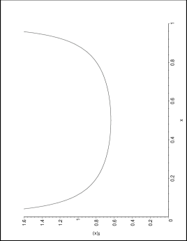
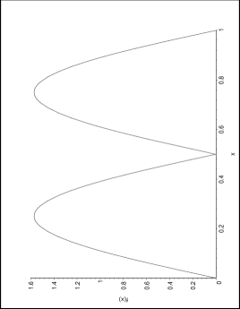
Figure 1: Graph of the density in Examples 5.5 (left) and 5.7 (right).

Remark 5.6.

The rate of convergence in Theorem 5.1 depends on $f$. From the proof of Theorem 5.1, it follows that for sufficiently large $n$,

$$p_{n}(F)\approx\frac{f^{(k)}(\mathsf{y}_{1}^{+})\,f^{(\ell)}(\mathsf{y}_{2}^{-})}{\left[f^{(k)}(\mathsf{y}_{1}^{+})+2^{-(k+1)}\,f^{(k)}\left(\frac{\mathsf{y}_{1}+\mathsf{y}_{2})}{2}^{+}\right)\right]\,\left[f^{(\ell)}(\mathsf{y}_{2}^{-})+2^{-(\ell+1)}\,f^{(\ell)}\left(\frac{(\mathsf{y}_{1}+\mathsf{y}_{2})}{2}^{-}\right)\right]}+\frac{c(f)}{n^{m}},$$

where

$$c(f)=\frac{s_{1}\,s_{3}^{\frac{1}{k+1}}\,\Gamma\left(\frac{\ell+2}{\ell+1}\right)+s_{2}\,s_{4}^{\frac{1}{\ell+1}}\,\Gamma\left(\frac{k+2}{k+1}\right)}{(k+1)\,(\ell+1)\,s_{3}^{\frac{k+2}{k+1}}\,s_{4}^{\frac{\ell+2}{\ell+1}}}$$

with $\Gamma(x)=\int_{0}^{\infty}\exp(-t)t^{(x-1)}\,dt$ and

$$s_{1} =\frac{1}{n^{\frac{k+\ell+1}{\ell+1}}}\,\frac{(-1)^{\ell+1}}{k!\,(\ell+1)!}\,f^{(k)}(\mathsf{y}_{1}^{+})\,f^{(\ell+1)}(\mathsf{y}_{2}^{-}), s_{3} =\frac{1}{(k+1)!}\left(f^{(k)}(\mathsf{y}_{1}^{+})+2^{-(k+1)}\,f^{(k)}\left(\frac{(\mathsf{y}_{1}+\mathsf{y}_{2})}{2}^{+}\right)\right),$$

$$s_{2} =\frac{1}{n^{\frac{k+\ell+1}{k+1}}}\,\frac{(-1)^{\ell}}{l!\,(k+1)!}\,f^{(k+1)}(\mathsf{y}_{1}^{+})\,f^{(\ell)}(\mathsf{y}_{2}^{-}), s_{4} =\frac{(-1)^{\ell+1}}{(\ell+1)!}\left(f^{(\ell)}(\mathsf{y}_{2}^{-})+2^{-(\ell+1)}\,f^{(\ell)}\left(\frac{(\mathsf{y}_{1}+\mathsf{y}_{2})}{2}^{-}\right)\right),$$

provided the derivatives exist. $\square$

Example 5.7.

Consider the distribution with absolute sine density $f(x)=\pi/2\,|\sin(2\,\pi\,x)|\;\mathbf{I}(0<x<1).$ See Figure 2 (right) for the plot of $f(x)$. Then $\mathcal{Y}_{2}=\{0,1\}$ and since $f(0^{+})=f\left(\frac{1}{2}^{+}\right)=0$ and $f(1^{-})=f\left(\frac{1}{2}^{-}\right)=0$ and $f^{\prime}(0)=f^{\prime}\left(\frac{1}{2}^{+}\right)=\pi^{2}$ and $f^{\prime}(1^{-})=f^{\prime}\left(\frac{1}{2}^{-}\right)=-\pi^{2}$, we apply Theorem 5.1 with $k=\ell=1$. Then $\lim_{n\rightarrow\infty}p_{n}(F)=16/25=0.64$. The numerically computed value (by numerical integration) of $p_{1000}(F)$ is $\widehat{p}_{1000}(F)\approx 0.6400$. $\square$

The distribution of $\gamma_{n}(F)$ depends on the distribution of $r(X_{i})=\min(d(X_{i},\mathsf{y}_{1}),\,d(X_{i},\mathsf{y}_{2}))$. Based on this, we have the following symmetry result.

Proposition 5.8.

Let $F_{1}$ and $F_{2}$ be two distributions with support $\mathcal{S}(F_{j})\subseteq(\mathsf{y}_{1},\mathsf{y}_{2})$ for $j=1,2$ such that $F_{1}(\mathsf{y}_{1}+x)=1-F_{2}\,(\mathsf{y}_{2}-x)$ for all $x\in(0,\mathsf{y}_{2}-\mathsf{y}_{1})$ (hence $f_{1}(\mathsf{y}_{1}+x)=f_{2}\,(\mathsf{y}_{2}-x)$). Also, let $\mathcal{X}^{j}_{n}$ be a set of iid random variables from $F_{j}$ for $j=1,2$. Then the distributions of $\gamma_{n}(F_{j})$ are identical for $j=1,2$.

Proof: By the change of variable $X=\varphi(U)=\mathsf{y}_{2}-\mathsf{y}_{1}-U$ for $U\in(0,\mathsf{y}_{2}-\mathsf{y}_{1})$, we get $F_{2}\,(\mathsf{y}_{1}+u)=1-F_{1}(\mathsf{y}_{2}-u)$. Furthermore, $\varphi(u)$ transforms $\Gamma_{1}(\mathcal{X}^{1}_{n},N_{\mathcal{Y}})$ into $\Gamma_{1}(\mathcal{X}^{2}_{n},N_{\mathcal{Y}})$ for $\mathcal{X}^{2}_{n}$, so $P(\gamma_{n}(F_{j})=2)$ are same for both $j=1,2$. Hence the desired result follows. $\blacksquare$

Below are asymptotic distributions of $\gamma_{n}(F)$ for various families of distributions. Recall that $p_{F}=\lim_{n\rightarrow\infty}p_{n}(F)=\lim_{n\rightarrow\infty}P\bigl{(}\gamma_{n}(F)=2\bigr{)}$. The asymptotic distribution of $\gamma_{n}(F)$ is $1+\operatorname{Bernoulli}\bigr{(}p_{F}\bigl{)}$. For the piecewise constant functions in Section 4.2.1, Theorem 5.1 applies. See Section 6.1 in Ceyhan, (2004).

Example 5.9.

Consider the distribution $F$ with density $f(\cdot)$ which is of the form

$$f(x)=(a\,x+b)\,\mathbf{I}\bigl{(}x\in(0,1)\bigr{)}\text{ with }|a|\leq 2,\;b=1-a/2.$$

So $k=\ell=0$ and $f(0^{+})=b$, $f(1^{-})=a+b$ and $f\left(\frac{1}{2}^{+}\right)=f\left(\frac{1}{2}^{-}\right)=a/2+b$. Then by Theorem 5.1, we have

$$\lim_{n\rightarrow\infty}p_{n}(F)=\frac{4-a^{2}}{9-a^{2}}=:p_{F}(a).$$

Note that $p_{F}(a)\in[0,4/9]$ is continuous in $a$ and decreases as $|a|$ increases. If $a=0$, then $F=\mathcal{U}(0,1)$, and $p_{F}(a=0)=4/9$. Moreover, $p_{F}(a=\pm 2)=0$; that is, for $a=\pm 2$, the asymptotic distribution of $\gamma_{n}(F)$ is degenerate. $\square$

Example 5.10.

Consider the normal distribution $\mathcal{N}(\mu,\sigma^{2})$ restricted to the interval $(0,1)$ with $\mu\in\mathbb{R}$ and $\sigma>0$. Then the corresponding density function is given by

$$f(x,\mu,\sigma)=\kappa\left(\frac{1}{\sqrt{2\pi}\,\sigma}\right)\exp\left(-\frac{(x-\mu)^{2}}{2\,\sigma^{2}}\right)\;\mathbf{I}(0<x<1),$$

where $\kappa=\left[\Phi\left(\frac{1-\mu}{\sigma}\right)-\Phi\left(\frac{-\mu}{\sigma}\right)\right]^{-1}$ with $\Phi(\cdot)$ being the cdf of the standard normal distribution $\mathcal{N}(0,1)$. Note that $k=\ell=0$, then by Theorem 5.1

$$\lim_{n\rightarrow\infty}p_{n}(F)=\frac{4}{\left(2+\exp\left(\frac{4\,\mu-1}{8\,\sigma^{2}}\right)\right)\left(2+\exp\left(\frac{3-4\,\mu}{8\,\sigma^{2}}\right)\right)}=:p_{F}(\mu,\sigma).$$

Observe that $p_{F}(\mu,\sigma)\in[0,4/9)$ is continuous in $\mu$ and $\sigma$ and increases as $\sigma$ increases for fixed $\mu$. Furthermore, for fixed $\mu$, $\lim_{\sigma\rightarrow\infty}p_{F}(\mu,\sigma)=4/9$ and $\lim_{\sigma\rightarrow 0}p_{F}(\mu,\sigma)=0$. For fixed $\sigma>0$, $\lim_{\mu\rightarrow\pm\infty}p_{F}(\mu,\sigma)=0$, $p_{F}(\mu,\sigma)$ decreases as $|\mu-1/2|$ increases, and $p_{F}(\mu,\sigma)$ is maximized at $\mu=1/2$. $\square$

Example 5.11.

Consider the distribution $F$ with density $f(\cdot)$ which is of the form

$$f(x)=2^{q}(q+1)\,\left[x^{q}\,\mathbf{I}\bigl{(}0<x<1/2\bigr{)}+(x-1/2)^{q}\,\mathbf{I}\bigl{(}1/2\leq x<1\bigr{)}\right]\text{ with }q\in[0,\infty].$$

See Figure 2 (left) with $q=2$. Since $f(0^{+})=f\left(\frac{1}{2}^{+}\right)=0$, we can apply Theorem 5.1 with $k=q$ and $l=0$. Then $f^{(q)}(0^{+})=(q+1)!\,2^{q}$, $f(1^{-})=(q+1)$, $f\left(\frac{1}{2}^{-}\right)=(q+1)$, and $f^{(q)}\,\left(\frac{1}{2}^{+}\right)=(q+1)!\,2^{q}$. By Theorem 5.1, we have

$$\lim_{n\rightarrow\infty}p_{n}(F)=\frac{2^{q+2}}{3\,(1+2^{q+1})}=:p_{F}(q).$$

Note that $p_{F}(q)\in[4/9,2/3]$ is a continuous increasing function of $q$. If $q=0$, then $F=\mathcal{U}(0,1)$. $\square$

Example 5.12.

Consider the distribution $F$ with density $f(\cdot)$ which is of the form

$$f(x)=\left(\delta+12\,(1-\delta)\,x^{2}\right)\,\mathbf{I}\bigl{(}0<x<1/2\bigr{)}+\left(\delta+12\,(1-\delta)\,(x-1/2)^{2}\right)\,\mathbf{I}\bigl{(}1/2\leq x<1\bigr{)}\text{ with }\delta\in[0,1].$$

See Figure 2 with $\delta=0$ (left) and $\delta=2/3$ (right). Since $f(0^{+})=\delta$, $f\,(1^{-})=(3-2\,\delta)$, $f\left(\frac{1}{2}^{-}\right)=(3-2\,\delta)$, and $f\left(\frac{1}{2}^{+}\right)=\delta$, for $\delta\in(0,1]\}$ we have $k=\ell=0$ and so by Theorem 5.1

$$\lim_{n\rightarrow\infty}p_{n}(F)=4/9\text{ for $\delta\in(0,1]$}.$$

Note that if $\delta=1$, then $F=\mathcal{U}(0,1)$. For $\delta=0$, we can apply Theorem 5.1 with $k=2$ and $l=0$. Hence we get $p_{F}(\delta=0)=16/27$. Observe that in this example, $\gamma_{n}(F)$ has two distinct non-degenerate distributions at different values of $\delta$. $\square$

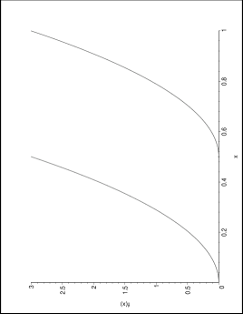
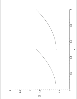
Figure 2: Left plot is for the density in Example 5.11 with $q=2$ or for the density in Example 5.12 with $\delta=0$. Right plot is for the density in Example 5.12 with $\delta=2/3$.

Remark 5.13.

If, in Theorem 5.1, we have $f^{(k)}(0^{+})=f^{(k)}\left(\frac{1}{2}^{+}\right)$ and $f^{(\ell)}(1^{-})=f^{(\ell)}\left(\frac{1}{2}^{-}\right)$, then

$$\lim_{n\rightarrow\infty}p_{n}(F)=\left(\frac{1}{1+2^{-(k+1)}}\right)\left(\frac{1}{1+2^{-(\ell+1)}}\right).$$

In particular, if $k=\ell=0$, then $\lim_{n\rightarrow\infty}p_{n}(F)=4/9$ (i.e., $\gamma_{n}(F)$ and $\gamma_{n}\bigl{(}\mathcal{U}(0,1)\bigr{)}$ have the same asymptotic distributions). $\square$

Example 5.14.

$\text{Beta}(\nu_{1},\nu_{2})$ with $\nu_{1},\nu_{2}\geq 1$. The density function is

$$f(x,{\nu_{1}},{\nu_{2}})={\frac{x^{\nu_{1}-1}(1-x)^{\nu_{2}-1}}{\beta(\nu_{1},\nu_{2})}}\;\mathbf{I}(0<x<1)\text{ where }\beta(\nu_{1},\nu_{2})=\frac{\Gamma(\nu_{1})\,\Gamma(\nu_{2})}{\Gamma(\nu_{1}+\nu_{2})}.$$

Then $\lim_{n\rightarrow\infty}p_{n}(\text{Beta}(\nu_{1},\nu_{2}))=0$ at rate $O\bigl{(}n^{-(\nu_{1}+\nu_{2}-2)}\bigr{)}$. Let $p_{n}(\nu_{1},\nu_{2})$ denote the $P\bigl{(}\gamma_{n}(F)=2\bigr{)}$ for $F=\text{Beta}(\nu_{1},\nu_{2})$. The numerically computed values of $p_{n}(\nu_{1},\nu_{2})$ for $n=1000$ are $\widehat{p}_{1000}(4,1)=\widehat{p}_{1000}(1,4)\approx 0.000005$, $\widehat{p}_{1000}(4,2)=\widehat{p}_{1000}(2,4)<0.00001$ and $\widehat{p}_{1000}(2,2)\approx 0.000001$. $\square$

Here is an example with general support $(\mathsf{y}_{1},\mathsf{y}_{2})$.

Example 5.15.

Consider the distribution $F$ with density $f(\cdot)$ which is of the form $f(x)=a\,x+b\text{ with }b=\frac{1}{(\mathsf{y}_{2}-\mathsf{y}_{1})}\bigl{(}1-a\,(\mathsf{y}_{2}^{2}-\mathsf{y}_{1}^{2})/2\bigr{)}\text{ and }|a|\leq\frac{2}{(\mathsf{y}_{2}-\mathsf{y}_{1})^{2}}.$ Using Theorem 5.1, we obtain $p_{F}=\frac{a^{2}\,(\mathsf{y}_{2}-\mathsf{y}_{1})^{4}-4}{a^{2}\,(\mathsf{y}_{2}-\mathsf{y}_{1})^{4}-9}$. If $(\mathsf{y}_{1},\mathsf{y}_{2})=(0,1)$, then $b=1-a/2$ and $p_{F}(a)=\frac{a^{2}-4}{a^{2}-9}$. In both cases, $p_{F}(a)$ is maximized for the uniform case; i.e., when $a=0$, then we have $p_{F}(a=0)=4/9$. Furthermore, $\gamma_{n}(F)$ is degenerate in the limit when $a=\pm\frac{2}{(\mathsf{y}_{2}-\mathsf{y}_{1})^{2}}$, since $p_{n}(F)\rightarrow 0$ as $n\rightarrow\infty$ at rate $O\bigl{(}n^{-1}\bigr{)}$. $\square$

For more detail and examples, see Sections 6.4 and 7.1 in Ceyhan, (2004).

6 The Distribution of the Domination Number of $\mathscr{D}_{n,m}$-digraphs

In this section, we attempt the more challenging case of $m>2$. For $c<d$ in $\mathbb{R}$, define the family of distributions

$$\mathscr{H}(\mathbb{R}):=\bigl{\{}F_{X,Y}:\;(X_{i},Y_{i})\sim F_{X,Y}\text{ with support }\mathcal{S}(F_{X,Y})=(c,d)^{2}\subsetneq\mathbb{R}^{2},\;\;X_{i}\sim F_{X}\text{ and }Y_{i}\stackrel{{\scriptstyle iid}}{{\sim}}F_{Y}\bigr{\}}.$$

We provide the exact distribution of $\gamma(D_{n,m})$ for $\mathscr{H}(\mathbb{R})$-random digraphs in the following theorem. Let $[m]:=\bigl{\{}0,1,\ldots,m-1\bigr{\}}$ and $\Theta^{S}_{a,b}:=\bigl{\{}(u_{1},\ldots u_{b}):\;\sum_{i=1}^{b}u_{i}=a:\;u_{i}\in S,\;\;\forall i\bigr{\}}$. Let $\mathcal{Y}_{m}=\bigl{\{}Y_{1},Y_{2},\ldots,Y_{m}\bigl{\}}$ whose order statistics are denoted as $Y_{(j)}$ for $j=1,2,\ldots,m$. Note that the order statistics are distinct a.s. provided $Y$ has a continuous distribution. Let $\gamma(D^{j})$ be the domination number of the digraph induced by $\mathcal{X}^{j}$ and $\mathcal{Y}^{j}$ (see Section 4). Given $Y_{(j)}=\mathsf{y}_{(j)}$ for $j=1,\ldots,m$, let $F_{j}$ be the (conditional) marginal distribution of $X$ restricted to $\mathcal{I}_{j}=\left(\mathsf{y}_{(j-1)},\mathsf{y}_{(j)}\right)$ for $j=1,\ldots,(m+1)$, $\vec{n}$ be the vector of numbers of $\mathcal{X}$ points $n_{j}$ falling into intervals $\mathcal{I}_{j}$. Let $f_{\vec{Y}}(\vec{\mathsf{y}})$ be the joint distribution of the order statistics of $\mathcal{Y}_{m}$, i.e., $f_{\vec{Y}}(\vec{\mathsf{y}})=\frac{1}{m!}\prod_{j=1}^{m}f(\mathsf{y}_{j})\,\mathbf{I}(c<\mathsf{y}_{1}<\ldots<\mathsf{y}_{m}<d)$, and $f_{j,k}(\mathsf{y}_{j},\mathsf{y}_{k})$ be the joint distribution of $Y_{(j)},Y_{(k)}$. Then we have the following theorem which is a generalization of the main result of Priebe et al., (2001).

Theorem 6.1.

Let $D$ be an $\mathscr{H}(\mathbb{R})$-random $\mathscr{D}_{n,m}$-digraph. Then the probability mass function of the domination number of D is given by

$$P(\gamma(D_{n,m})=k)=\int_{\mathscr{S}}\sum_{\vec{n}\in\Theta^{[n+1]}_{n,(m+1)}}\sum_{\vec{k}\in\Theta^{[3]}_{k,(m+1)}}P(\vec{N}=\vec{n})\,\zeta(k_{1},n_{1})\,\zeta(k_{m+1},\,n_{m+1})\prod_{j=2}^{m}\eta(k_{j},n_{j})f_{\vec{Y}}(\vec{\mathsf{y}})\,d\mathsf{y}_{1}\ldots d\mathsf{y}_{m}$$

where $P(\vec{N}=\vec{n})$ is the joint probability of $n_{j}$ points falling into intervals $\mathcal{I}_{j}$ for $j=1,2,\ldots,(m+1)$, $k_{j}\in\{0,1,2\}$, and

$$\zeta(k_{j},n_{j}) =\max\bigl{(}\mathbf{I}(n_{j}=k_{j}=0),\mathbf{I}(n_{j}\geq k_{j}=1)\bigr{)}\text{ for }j=1,(m+1),\text{ and }$$

$$\eta(k_{j},n_{j}) =\max\bigl{(}\mathbf{I}(n_{j}=k_{j}=0),\mathbf{I}(n_{j}\geq k_{j}\geq 1)\bigr{)}\cdot p_{n_{j}}(F_{j})^{\mathbf{I}(k_{j}=2)}\,\bigl{(}1-p_{n_{j}}(F_{j})\bigr{)}^{\mathbf{I}(k_{j}=1)}$$

for $$j=2,\ldots,m,$$ and the region of integration is given by

$$\mathscr{S}:=\bigl{\{} (\mathsf{y}_{1},\mathsf{y}_{2},\ldots,\mathsf{y}_{m})\in(c,d)^{2}:\,c<\mathsf{y}_{1}<\mathsf{y}_{2}<\ldots<\mathsf{y}_{m}<d\bigr{\}}.$$

Proof: For $\gamma(D_{n,m})=\sum_{j=1}^{m+1}\,\gamma(D^{j})=k$, we must have $\gamma(D^{j})=k_{j}$ for $j=1,\ldots,(m+1)$ so that $\sum_{j=1}^{m+1}\,k_{j}=k$ and $\sum_{j=1}^{m+1}n_{j}=n$. By definition, $\Theta^{[n+1]}_{n,(m+1)}$ is the collection of such $\vec{n}$ and since $k_{j}\in\{0,1,2\}$ for all $j=1,\ldots,(m+1)$, $\Theta^{[3]}_{k,(m+1)}$ is the collection of such $\vec{k}$. We treat the end intervals, $\mathcal{I}_{1}$ and $\mathcal{I}_{m+1}$, separately. The indicator functions in the statement of the theorem guarantees that the pairs $n_{j},k_{j}$ are compatible for $j\in\{1,(m+1)\}$; that is, incompatible pairs such as $(n_{j}=0,k_{j}>0)$ are eliminated. The $\zeta$ terms equal unity if $(n_{j},k_{j})$ are compatible. Therefore we have

$$P(\gamma(D_{n,m})=k)=\int_{\mathscr{S}}\sum_{\vec{n}\in\Theta^{[n+1]}_{n,(m+1)}}\sum_{\vec{k}\in\Theta^{[3]}_{k,(m+1)}}P(\vec{N}=\vec{n})\,\prod_{j=1}^{m+1}\eta(k_{j},n_{j})f_{\vec{Y}}(\vec{\mathsf{y}})\,d\mathsf{y}_{1}\ldots d\mathsf{y}_{m}\\ =\int_{\mathscr{S}}\sum_{\vec{n}\in\Theta^{[n+1]}_{n,(m+1)}}\sum_{\vec{k}\in\Theta^{[3]}_{k,(m+1)}}P(\vec{N}=\vec{n})\,\prod_{j\in\{1,(m+1)\}}\eta(k_{j},n_{j})\prod_{j=2}^{m}\eta(k_{j},n_{j})f_{\vec{Y}}(\vec{\mathsf{y}})\,d\mathsf{y}_{1}\ldots d\mathsf{y}_{m}\\ =\int_{\mathscr{S}}\sum_{\vec{n}\in\Theta^{[n+1]}_{n,(m+1)}}\sum_{\vec{k}\in\Theta^{[3]}_{k,(m+1)}}P(\vec{N}=\vec{n})\,\zeta(k_{1},n_{1})\,\zeta(k_{m+1},\,n_{m+1})\prod_{j=2}^{m}\eta(k_{j},n_{j})f_{\vec{Y}}(\vec{\mathsf{y}})\,d\mathsf{y}_{1}\ldots d\mathsf{y}_{m}$$

where we have used the conditional pairwise independence of $\gamma(D^{j})$. The $\eta$ terms are based on the compatibility of pairs $(n_{j},k_{j})$ for $j=1,\ldots,(m+1)$ and $p_{n_{j}}(F_{j})=P(\gamma(D^{j})=2)$. $\blacksquare$

For $n,m<\infty$, the expected value of domination number is

$$\mathbf{E}[\gamma(D_{n,m})]=P\left(X_{(1)}<Y_{(1)}\right)+P\left(X_{(n)}>Y_{(m)}\right)+\sum_{j=2}^{m}\sum_{k=1}^{n}\,P(N_{j}=k)\,\mathbf{E}[\gamma(D^{j})]$$ (13)

where

$$P(N_{j}=k)=\\ \int_{c}^{d}\int_{\mathsf{y}_{(j-1)}}^{d}f_{j-1,j}\left(\mathsf{y}_{(j-1)},\mathsf{y}_{(j)}\right)\Bigl{[}F_{X}\left(\mathsf{y}_{(j)}\right)-F_{X}\left(\mathsf{y}_{(j-1)}\right)\Bigr{]}^{k}\Bigl{[}1-\left(F_{X}\left(\mathsf{y}_{(j)}\right)-F_{X}\left(\mathsf{y}_{(j-1)}\right)\right)\Bigr{]}^{n-k}\,d\mathsf{y}_{(j)}d\mathsf{y}_{(j-1)}$$

and $\mathbf{E}[\gamma(D^{j})]=1+p_{k}(F_{j})$.

Corollary 6.2.

For $F_{X,Y}\in\mathscr{H}(\mathbb{R})$ with support $\mathcal{S}(F_{X})\cap\mathcal{S}(F_{Y})$ of positive measure, $\lim_{n\rightarrow\infty}\mathbf{E}[\gamma(D_{n,n})]=\infty$.

Proof: Consider the intersection of the supports $\mathcal{S}(F_{X})\cap\mathcal{S}(F_{Y})$ that has positive (Lebesgue) measure. For $\mathcal{S}(Y)\setminus\mathcal{S}(X)$; i.e., in the intervals $\mathcal{I}_{j}$ falling outside the intersection $\mathcal{S}(F_{X})\cap\mathcal{S}(F_{Y})$, the domination number of the component $D^{j}$ is $\gamma(D^{j})=0$ w.p. 1 but inside the intersection, $\gamma(D^{j})>0$ w.p. 1 for infinitely many $j$. That is,

$$\mathbf{E}[\gamma(D_{n,n})] = P\left(X_{(1)}<Y_{(1)}\right)+P(X_{(n)}>Y_{(n)})+\sum_{j=2}^{n}\sum_{k=1}^{n}\,P(N_{j}=k)\,\mathbf{E}[\gamma_{N_{j}}(F_{j})]$$

$$> \sum_{j=2}^{n}\sum_{k=1}^{n}\,P(N_{j}=k)\,\mathbf{E}[\gamma_{N_{j}}(F_{j})]=\sum_{j=2}^{n}\sum_{k=1}^{n}\,P(N_{j}=k)\,(1+p_{N_{j}}(F_{j}))$$

$$> \sum_{j=2}^{n}\sum_{k=1}^{n}\,P(N_{j}=k)>\sum_{j=2}^{n}\,P(N_{j}\geq 1)$$

$$\approx n\text{~{}~{}~{} (for sufficiently large $n$)}$$

where $\mathbf{E}[\gamma_{N_{j}}(F_{j})]=(1+p_{N_{j}}(F_{j}))$ follows from the fact that $\gamma_{N_{j}}(F_{j})\sim 1+\operatorname{Bernoulli}(p_{N_{j}}(F_{j}))$ from Theorem 4.2. Furthermore, $P(N_{j}\geq 1)\approx 1$ for sufficiently large $n$. Then the desired result follows. $\blacksquare$

Theorem 6.3.

Let $D_{n,m}$ be an $\mathscr{H}(\mathbb{R})$-random $\mathscr{D}_{n,m}$-digraph. Then (i) for fixed $n<\infty$, $\lim_{m\rightarrow\infty}\gamma(D_{n,m})=n$ a.s. (ii) for fixed $m<\infty$, $\lim_{n\rightarrow\infty}\gamma(D_{n,m})\stackrel{{\scriptstyle d}}{{=}}m+1+\sum_{j=1}^{m}B_{j}$, where $B_{j}\sim\operatorname{Bernoulli}(p_{F_{j}})$ where $\stackrel{{\scriptstyle d}}{{=}}$ stands for equality in distribution.

Proof: Part (i) is trivial. As for part (ii), first note that $N_{j}\rightarrow\infty$ as $n\rightarrow\infty$ for all $j$ a.s., hence $\lim_{n\rightarrow\infty}\gamma(D^{1})=\lim_{n\rightarrow\infty}\gamma(D^{m+1})=1$ a.s. and $\lim_{n\rightarrow\infty}\gamma(D^{j})=1+\operatorname{Bernoulli}(p_{F_{j}})$ a.s. for $j=2,\ldots,m$ where

$$p_{F_{j}}=\int_{c}^{d}\int_{\mathsf{y}_{(j-1)}}^{d}H^{*}\left(\mathsf{y}_{(j-1)},\mathsf{y}_{(j)}\right)\,f_{j-1,j}\left(\mathsf{y}_{(j-1)},\mathsf{y}_{(j)}\right)\,d\mathsf{y}_{(j)}d\mathsf{y}_{(j-1)}$$

with $H^{*}\left(\mathsf{y}_{(j-1)},\mathsf{y}_{(j)}\right)=\lim_{n_{j}\rightarrow\infty}(p_{n_{j}}(F_{j}))$ which is given in Theorem 6.1 for $F_{j}$ with density $f_{j}$ whose support is $\left(\mathsf{y}_{(j-1)},\mathsf{y}_{(j)}\right)$. Then the desired result follows. $\blacksquare$

So far, $\mathcal{Y}_{m}$ is assumed to be a random sample, so $P(\gamma(D_{n,m})=k)$ includes the integration with respect to $f_{\vec{Y}}(\vec{\mathsf{y}})$ which can be lifted by conditioning. Conditional on $\mathcal{Y}_{m}=\left\{\mathsf{y}_{(1)},\ldots,\mathsf{y}_{(m)}\right\}$, by Theorem 6.1 we have

$$P(\gamma(D_{n,m})=k)=\sum_{\vec{n}\in\Theta^{[n+1]}_{n,(m+1)}}\sum_{\vec{k}\in\Theta^{[3]}_{k,(m+1)}}P(\vec{N}=\vec{n})\,\zeta(k_{1},n_{1})\,\zeta(k_{m+1},\,n_{m+1})\prod_{j=2}^{m}\eta(k_{j},n_{j}),$$

where $\zeta(k_{j},n_{j})$ and $\eta(k_{j},n_{j})$ are as in Theorem 6.1; and the expected domination number $\mathbf{E}[\gamma(D_{n,m})]$ is as in Equation (13) with $P(N_{j}=k)=\left[F_{X}\left(\mathsf{y}_{(j)}\right)-F_{X}\left(\mathsf{y}_{(j-1)}\right)\right]^{k}\left[1-\left(F_{X}\left(\mathsf{y}_{(j)}\right)-F_{X}\left(\mathsf{y}_{(j-1)}\right)\right)\right]^{n-k}$; and $\lim_{n\rightarrow\infty}\gamma(D_{n,m})\stackrel{{\scriptstyle d}}{{=}}m+1+\sum_{j=1}^{m}B_{j}$, where $B_{j}\sim\operatorname{Bernoulli}(p_{F_{j}})$ with $p_{F_{j}}:=\lim_{n_{j}\rightarrow\infty}p_{n_{j}}(F_{j})$.

Let $F_{X}$ be a distribution with support $\mathcal{S}(F_{X})\subseteq(0,1)$ and density $f_{X}(x)$. Conditional on $\mathcal{Y}_{m}=\left\{\mathsf{y}_{(1)},\ldots,\mathsf{y}_{(m)}\right\}$, let $F_{j}$ be the distribution with density $f_{j}(x)=\frac{1}{\left(\mathsf{y}_{(j)}-\mathsf{y}_{(j-1)}\right)}f_{X}\left(\frac{x-\mathsf{y}_{(j-1)}}{\mathsf{y}_{(j)}-\mathsf{y}_{(j-1)}}\right)$ for $j=2,\ldots,m$, and $\mathcal{S}(F_{j}(x))$ is non-empty for $j\in\{1,(m+1)\}$. By this construction, the independence of the distribution of $\gamma_{n}(F_{j})$ from $\mathcal{I}_{j}$ obtains; i.e., $\gamma_{n}(F_{j})\stackrel{{\scriptstyle d}}{{=}}\gamma_{n}(F_{X})$ for all $j\in\{1,\ldots,(m+1)\}$. Now consider the family $\mathscr{H}_{\mathcal{U}}(\mathbb{R})$ defined as

$$\mathscr{H}_{\mathcal{U}}(\mathbb{R}):=\bigl{\{}F_{X,Y}:(X_{i},Y_{i})\sim F_{X,Y},\;Y_{j}\stackrel{{\scriptstyle iid}}{{\sim}}\mathcal{U}(c,d)\text{ for }(c,d)\subsetneq\mathbb{R},\text{ and }X_{i}|\mathcal{Y}_{m}\stackrel{{\scriptstyle iid}}{{\sim}}F_{j}\bigr{\}}.$$

Clearly $\mathscr{H}_{\mathcal{U}}(\mathbb{R})\subsetneq\mathscr{H}(\mathbb{R})$.

Corollary 6.4.

Suppose $F_{X,Y}\in\mathscr{H}_{\mathcal{U}}(\mathbb{R})$. Then

$$P(\gamma(D_{n,m})=k)=\sum_{\vec{n}\in\Theta^{[n+1]}_{n,(m+1)}}\sum_{\vec{k}\in\Theta^{[3]}_{k,(m+1)}}P(\vec{N}=\vec{n})\,\zeta(k_{1},n_{1})\,\zeta(k_{m+1},\,n_{m+1})\prod_{j=2}^{m}\eta(k_{j},n_{j})$$

where $\zeta(k_{j},n_{j})$ and $\eta(k_{j},n_{j})$ are as in Theorem 6.1.

Note that if in addition, $P_{F_{j}}(X\in\mathcal{I}_{j})=P_{\mathcal{U}}(X\in\mathcal{I}_{j})$ for all $j$, then $P(\vec{N}=\vec{n})={n+m\choose n}^{-1}$, since each $\vec{n}\in\Theta^{[n+1]}_{n,(m+1)}$ occurs with probability ${n+m\choose n}^{-1}$. Moreover, $F=\mathcal{U}(c,d)$ is a special case of Corollary 6.4. For $n,m<\infty$, we have the explicit form of $p_{n_{j}}(F_{j})$ for $F_{j}$ with piecewise constant density $f_{j}$.

Here are some examples which are generalized from piecewise-constant densities so that now the distribution of $\gamma(D^{j})$ is independent from the support $(\mathsf{y}_{(j-1)},\mathsf{y}_{(j)})$. Hence Corollary 6.4 applies to these examples.

Example 6.5.

• Let $u_{j}:=\frac{\bigl{(}\mathsf{y}_{(j-1)}+\mathsf{y}_{(j)}\bigr{)}}{2}$ and $v_{j}:=\mathsf{y}_{(j)}-\mathsf{y}_{(j-1)}$.

• If $f(\cdot)$ is of the form

  $$f(x)=\frac{1}{(1-2\,\delta)\,v_{j}}\,\mathbf{I}\left(x\in\left(\mathsf{y}_{(j-1)}+\delta\,v_{j},\mathsf{y}_{(j)}-\delta\,v_{j}\right)\right)\text{ with }\delta\in[0,1/3]$$

  then $p_{n}(F)$ is as in Equation (7).

• If $f(\cdot)$ is of the form

  $$f(x)=\frac{1}{(1-2\,\delta)\,v_{j}}\,\mathbf{I}\left(x\in\left(\mathsf{y}_{(j-1)},u_{j}-\delta\,v_{j}\right)\cup\left[u_{j}+\delta\,v_{j},\mathsf{y}_{(j)}\right)\right)\text{ with }\delta\in[0,1/3],$$

  then $p_{n}(F)$ is as in Equation (8).

• If $f(\cdot)$ is of the form

  $$f(x)=\frac{(1+\delta)}{\,v_{j}}\,\mathbf{I}\left(x\in\left(\mathsf{y}_{(j-1)},u_{j}\right)\right)+\frac{(1-\delta)}{\,v_{j}}\,\mathbf{I}\left(x\in\left[u_{j},\mathsf{y}_{(j)}\right)\right),$$

  then $p_{n}(F)$ is as in Equation (9).

• If $f(\cdot)$ is of the form

  $$f(x)=f_{1}(x)\,\mathbf{I}\left(x\in\left(\mathsf{y}_{(j-1)},t_{j}\right)\right)+f_{2}\,(x)\,\mathbf{I}\left(x\in\left[t_{j},w_{j}\right)\right)+f_{3}\,(x)\,\mathbf{I}\left(x\in\left[w_{j},\mathsf{y}_{(j)}\right)\right)$$

  where $t_{j}=\frac{\mathsf{y}_{(j)}+3\,\mathsf{y}_{(j-1)}}{4}$, $w_{j}=\frac{3\mathsf{y}_{(j)}+\mathsf{y}_{(j-1)}}{4}$, $f_{1}(x)=\frac{(1+\delta)}{\,v_{j}}$, $f_{2}\,(x)=\frac{(1-\delta)}{\,v_{j}}$ and $f_{3}\,(x)=\frac{(1+\delta)}{\,v_{j}}$, then $p_{n}(F)$ is as in Example 4.9. $\square$

Theorem 6.6.

Let $D$ be an $\mathscr{H}_{\mathcal{U}}(\mathbb{R})$-random $\mathscr{D}_{n,m}$-digraph with the additional assumption that $P_{F_{j}}(X\in\mathcal{I}_{j})=P_{\mathcal{U}}(X\in\mathcal{I}_{j})$ for all $j$. Then

$$\mathbf{E}[\gamma(D_{n,m})]=\frac{2\,n}{n+m}+\frac{n!\,m\,(m-1)}{(n+m)!}\,\sum_{i=1}^{n}\frac{(n+m-i-1)!}{(n-i)!}\,(1+p_{i}(F))$$

where $p_{i}(F)=P(\gamma(D_{i,2})=2)$.

Proof: Similar to the Proof of Theorem 4 in Priebe et al., (2001). $\blacksquare$

Furthermore, from Corollary 6.2, we have $\mathbf{E}[\gamma(D_{n,n})]\rightarrow\infty$ as $n\rightarrow\infty$.

Theorem 6.7.

Let $D_{n,m}$ be an $\mathscr{H}_{\mathcal{U}}(\mathbb{R})$-random $\mathscr{D}_{n,m}$-digraph. Then (i) for fixed $n<\infty$, $\lim_{m\rightarrow\infty}\gamma(D_{n,m})=n$ a.s. (ii) for fixed $m<\infty$, $\lim_{n\rightarrow\infty}\gamma(D_{n,m})\stackrel{{\scriptstyle d}}{{=}}m+1+B$, where $B\sim Binomial(m-1,p_{F})$ where $p_{F}=\lim_{n\rightarrow\infty}P(\gamma(D_{n,2})=2)$.

Proof: Similar to the Proof of Theorem 5 in Priebe et al., (2001). $\blacksquare$

Remark 6.8.

Extension to Multi-dimensional Case: The existence of ordering of points in $\mathbb{R}$ is crucial in our calculations. The order statistics of $\mathcal{Y}_{m}$ partition the support $(c,d)$ into disjoint intervals a.s. which can also be viewed as the Delaunay tessellation of $\mathbb{R}$ based on $\mathcal{Y}_{m}$. This nice structure in $\mathbb{R}$ avails a minimum dominating set and hence the domination number, both in polynomial time. Furthermore, the $\Gamma_{1}$-region is readily available by the order statistics of $\mathcal{X}_{n}$; also the components of the digraph restricted to intervals $\mathcal{I}_{j}$ (see Section 4) are not connected to each other, since $N_{\mathcal{Y}}(x)\cap N_{\mathcal{Y}}(y)=\emptyset$ for $x,\,y$ in distinct intervals. The straightforward extension to multiple dimensions (i.e., $\mathbb{R}^{d}$ with $d>1$) does not have a nice ordering structure; and $\mathcal{Y}_{m}$ does not readily partition the support, but we can use the Delaunay tessellation based on $\mathcal{Y}_{m}$. Furthermore, in multiple dimensions finding a minimum dominating set is an NP-hard problem; and $\Gamma_{1}$-regions are not readily available (in fact for $n_{j}>3$, complexity of finding the $\Gamma_{1}$-regions is an open problem). In addition, in multiple dimensions the components of the digraph restricted to Delaunay cells are not necessarily disconnected from each other, since $N_{\mathcal{Y}}(x)\cap N_{\mathcal{Y}}(y)\not=\emptyset$ might hold for $x,\,y$ in distinct Delaunay cells. These have motivated us to generalize the proximity map $N_{\mathcal{Y}}$ in order to avoid the difficulties above. See Ceyhan and Priebe, (2003, 2005), where two new families of proximity maps are introduced, and the generalization of CCCD are called proximity catch digraphs. The distribution of the domination number of these proximity maps is still a topic of ongoing research. $\square$

7 Discussion

This article generalizes the main result of Priebe et al., (2001) in several directions. Priebe et al., (2001) provided the exact (finite sample) distribution of the class cover catch digraphs (CCCDs) based on $\mathcal{X}_{n}$ and $\mathcal{Y}_{m}$ both of which were sets of iid random variables from a uniform distribution on $(c,d)\subset\mathbb{R}$ with $-\infty<c<d<\infty$ and the proximity map $N_{\mathcal{Y}}(x):=B(x,r(x))$ where $r(x):=\min_{\mathsf{y}\in\mathcal{Y}_{m}}d(x,\mathsf{y})$. First, given $\mathcal{Y}_{2}=\{\mathsf{y}_{1},\mathsf{y}_{2}\}\subset\mathbb{R}$, we lift the uniformity assumption of $\mathcal{X}_{n}$ by assuming it to be from a non-uniform distribution $F$ with support $\mathcal{S}(F)\subseteq(\mathsf{y}_{1},\mathsf{y}_{2})$. The exact distribution of the domination number of the associated CCCD, $\gamma_{n}(F)$, is calculated for $F$ that has piecewise constant density $f$ on $(\mathsf{y}_{1},\mathsf{y}_{2})$. For more general $F$, the exact distribution is not analytically available in simple closed form, so we compute it by numerical integration. However, the asymptotic distribution of $\gamma_{n}(F)$ is tractable, which is the one of the main results of this article. Unfortunately, the distribution of $\gamma_{n}(F)$ depends on $\mathcal{Y}_{2}$, hence the distribution of the domination number of a CCCD, $\gamma(D_{n,m})$, for $\mathcal{X}_{n}$ and $\mathcal{Y}_{m}$ with $m>2$, for general $F$ includes integration with respect to order statistics of $\mathcal{Y}_{m}$. We provide the conditions that make $\gamma(D_{n,m})$ independent of $\mathcal{Y}_{m}$. As another generalization direction, we also devise proximity maps depending on $F$ that will yield the distribution identical to that of $\gamma_{n}(\mathcal{U}(\mathsf{y}_{1},\mathsf{y}_{2}))$. Our set-up is more general than the one given in Priebe et al., (2001). The definition of the proximity map is generalized to any probability space and is only assumed to have a regional relationship to determine the inclusion of a point in the proximity region.

The exact (finite sample) distribution of $\gamma_{n}(F)$ characterizes $F$ up to a special type of symmetry (see Proposition 5.8). Furthermore, this article will form the foundation of the generalizations and calculations for uniform and non-uniform cases in multiple dimensions. As in Ceyhan and Priebe, (2005), we can use the domination number in testing one-dimensional spatial point patterns and our results will help make the power comparisons possible for large families of distributions.

References

Ceyhan, (2004)
Ceyhan, E. (2004).
The distribution of the domination number of class cover catch
digraphs for non-uniform one-dimensional data.
Technical Report 646, Department of Applied Mathematics and
Statistics, The Johns Hopkins University, Baltimore, MD, 21218.
Ceyhan and Priebe, (2003)
Ceyhan, E. and Priebe, C. (2003).
Central similarity proximity maps in Delaunay tessellations.
In Proceedings of the Joint Statistical Meeting, Statistical
Computing Section, American Statistical Association.
Ceyhan and Priebe, (2005)
Ceyhan, E. and Priebe, C. E. (2005).
The use of domination number of a random proximity catch digraph for
testing spatial patterns of segregation and association.
Statistics and Probability Letters, 73:37–50.
Chartrand and Lesniak, (1996)
Chartrand, G. and Lesniak, L. (1996).
Graphs & Digraphs.
Chapman & Hall/CRC Press LLC, Florida.
DeVinney et al., (2002)
DeVinney, J., Priebe, C. E., Marchette, D. J., and Socolinsky, D. (2002).
Random walks and catch digraphs in classification.
http://www.galaxy.gmu.edu/interface/I02/I2002Proceedings/DeVinneyJason/%DeVinneyJason.paper.pdf.
Proceedings of the Symposium on the Interface: Computing Science
and Statistics, Vol. 34.
DeVinney and Wierman, (2003)
DeVinney, J. and Wierman, J. C. (2003).
A SLLN for a one-dimensional class cover problem.
Statistics and Probability Letters, 59(4):425–435.
Janson et al., (2000)
Janson, S., Łuczak, T., and Rucinński, A. (2000).
Random Graphs.
Wiley-Interscience Series in Discrete Mathematics and Optimization,
John Wiley & Sons Inc., New York.
Jaromczyk and Toussaint, (1992)
Jaromczyk, J. W. and Toussaint, G. T. (1992).
Relative neighborhood graphs and their relatives.
Proceedings of IEEE, 80:1502–1517.
Marchette and Priebe, (2003)
Marchette, D. J. and Priebe, C. E. (2003).
Characterizing the scale dimension of a high dimensional
classification problem.
Pattern Recognition, 36(1):45–60.
Priebe et al., (2001)
Priebe, C. E., DeVinney, J. G., and Marchette, D. J. (2001).
On the distribution of the domination number of random class catch
cover digraphs.
Statistics and Probability Letters, 55:239–246.
(11)
Priebe, C. E., Marchette, D. J., DeVinney, J., and Socolinsky, D. (2003a).
Classification using class cover catch digraphs.
Journal of Classification, 20(1):3–23.
(12)
Priebe, C. E., Solka, J. L., Marchette, D. J., and Clark, B. T. (2003b).
Class cover catch digraphs for latent class discovery in gene
expression monitoring by DNA microarrays.
Computational Statistics and Data Analysis on Visualization,
43-4:621–632.
Prisner, (1994)
Prisner, E. (1994).
Algorithms for interval catch digraphs.
Discrete Applied Mathematics, 51:147–157.
Sen et al., (1989)
Sen, M., Das, S., Roy, A., and West, D. (1989).
Interval digraphs: An analogue of interval graphs.
Journal of Graph Theory, 13:189–202.
Tuza, (1994)
Tuza, Z. (1994).
Inequalities for minimal covering sets in sets in set systems of
given rank.
Discrete Applied Mathematics, 51:187–195.
West, (2001)
West, D. B. (2001).
Introduction to Graph Theory, Ed.Prentice Hall, N.J.