Matrix solutions of a noncommutative KP equation and a noncommutative mKP equation

Abstract

Matrix solutions of a noncommutative KP and a noncommutative mKP equation which can be expressed as quasideterminants are discussed. In particular, we investigate interaction properties of two-soliton solutions.

1 Introduction

A considerable amount of literature exists concerning noncommutative integrable systems. This includes noncommutative versions of the Burgers equation, the KdV equation, the KP equation, the mKP equation and the sine-Gordon equation [6, 14, 15, 2, 19, 8, 5, 12, 11, 1]. These equations can often be obtained by simply removing the assumption that the dependent variables and their derivatives in the Lax pair commute.

This paper is concerned with a noncommutative KP equation (ncKP) and a noncommutative mKP equation (ncmKP) [19, 13]. The Lax pair for ncKP is given by

$$L_{\scriptscriptstyle\textrm{KP}} =\partial_{x}^{2}+v_{x}-\partial_{y},$$ (1)

$$M_{\scriptscriptstyle\textrm{KP}} =4\partial_{x}^{3}+6v_{x}\partial_{x}+3v_{xx}+3v_{y}+\partial_{t}.$$ (2)

Both $L_{\scriptscriptstyle\textrm{KP}}$ and $M_{\scriptscriptstyle\textrm{KP}}$ are covariant under the Darboux transformation
$G_{\theta}=\theta\partial_{x}\theta^{-1}$, where $\theta$ is an eigenfunction for $L_{\scriptscriptstyle\textrm{KP}},M_{\scriptscriptstyle\textrm{KP}}$. From the compatibility condition $[L_{\scriptscriptstyle\textrm{KP}},M_{\scriptscriptstyle\textrm{KP}}]=0$ we obtain a noncommutative version of the KP equation:

$$(v_{t}+3v_{x}v_{x}+v_{xxx})_{x}+3v_{yy}+3[v_{x},v_{y}]=0,$$ (3)

where $u=v_{x}$. For ncmKP, the Lax pair [19] is given by

$$L_{\scriptscriptstyle\textrm{mKP}} =\partial_{x}^{2}+2w\partial_{x}-\partial_{y},$$ (4)

$$M_{\scriptscriptstyle\textrm{mKP}} =4\partial_{x}^{3}+12w\partial_{x}^{2}+6(w_{x}+w^{2}+W)\partial_{x}+\partial_{t}.$$ (5)

Both $L_{\scriptscriptstyle\textrm{mKP}}$ and $M_{\scriptscriptstyle\textrm{mKP}}$ are covariant under the Darboux transformation
$G_{\theta}=((\theta^{-1})_{x})^{-1}\partial_{x}\theta^{-1}$, where $\theta$ is an eigenfunction for $L_{\scriptscriptstyle\textrm{mKP}},M_{\scriptscriptstyle\textrm{mKP}}$. The compatibility condition $[L_{\scriptscriptstyle\textrm{mKP}},M_{\scriptscriptstyle\textrm{mKP}}]=0$ gives

$$0 =w_{t}+w_{xxx}-6ww_{x}w+3W_{y}+3[w_{x},W]_{+}-3[w_{xx},w]-3[W,w^{2}],$$ (6)

$$0 =W_{x}-w_{y}+[w,W].$$ (7)

Equations (6) and (7) form a noncommutative version of the mKP equation. Equation (7) is satisfied identically by applying the change of variables [19]

$$w=-f_{x}f^{-1},\quad W=-f_{y}f^{-1}.$$ (8)

The change of variables (8) has also been used in [6, 2] to study a noncommutative mKP hierarchy. For both ncKP and ncmKP equations, we consider families of solutions obtained from iterating binary Darboux transformations. These solutions can be expressed as quasideterminants, which were introduced by Gelfand et al in [4]. An $n\times n$ matrix $Z=(z_{ij})_{n\times n}$ over a ring $\mathcal{R}$ (noncommutative, in general) has $n^{2}$ quasideterminants, each of which is denoted $|Z|_{ij}$ for $1\leq i,j\leq n$. Let $r_{i}^{j}$ denote the row vector obtained from the $i$th row of $Z$ be deleting the $j$th entry, let $c_{j}^{i}$ denote the column vector obtained from the $j$th row of $Z$ by deleting the $i$th entry, let $Z^{ij}$ be the matrix obtained from $Z$ by deleting the $i$th row and $j$th column and assume that $Z^{ij}$ is invertible. Then $|Z|_{ij}$ exists and

$$|Z|_{ij} =z_{ij}-r_{i}^{j}(Z^{ij})^{-1}c_{j}^{i}.$$ (9)

For notational convenience, we box the leading element about which the expansion is made so that

$$|Z|_{ij} =\begin{vmatrix}Z^{ij}&c_{j}^{i}\\ r_{i}^{j}&\framebox{$z_{ij}$}\end{vmatrix}.$$ (10)

The quasideterminant solutions obtained from binary Darboux transformations reduce to ratios of grammian determinants in the commutative limit and we call them quasigrammians.

In this paper, we will consider the case where the dependent variables in ncKP and ncmKP are matrices and apply the methods used in [8, 9, 10, 7]. From this platform, we investigate the interaction of the two-soliton solution of the matrix versions of ncKP and ncmKP.

2 Quasigrammian solutions of the ncKP equation

In this section we recall the construction of the quasigrammian solutions of ncKP in [5]. The adjoint Lax pair is

$$L_{\scriptscriptstyle\textrm{KP}}^{{\dagger}} =\partial_{x}^{2}+v_{x}^{{\dagger}}+\partial_{y},$$ (11)

$$M_{\scriptscriptstyle\textrm{KP}}^{{\dagger}} =-4\partial_{x}^{3}-6v_{x}^{{\dagger}}\partial_{x}-3v_{xx}^{{\dagger}}+3v_{y}^{{\dagger}}-\partial_{t}.$$ (12)

Following the standard construction of a binary Darboux transformation (see [16]), one introduces a potential $\Omega(\phi,\psi)$ satisfying

$$\Omega(\phi,\psi)_{x} =\psi^{{\dagger}}\phi,\quad\Omega(\phi,\psi)_{y}=\psi^{{\dagger}}\phi_{x}-\psi_{x}^{{\dagger}}\phi,$$

$$\Omega(\phi,\psi)_{t} =-4(\psi^{{\dagger}}\phi_{xx}-\psi_{x}^{{\dagger}}\phi_{x}+\psi_{xx}^{{\dagger}}\phi)-6\psi^{{\dagger}}v_{x}\phi.$$

The parts of this definition are compatible when $L_{\scriptscriptstyle\textrm{KP}}[\phi]=M_{\scriptscriptstyle\textrm{KP}}[\phi]=0$ and $L_{\scriptscriptstyle\textrm{KP}}^{{\dagger}}[\psi]=M_{\scriptscriptstyle\textrm{KP}}^{{\dagger}}[\psi]=0$. Note that we can define $\Omega(\Phi,\Psi)$ for any row vectors $\Phi$ and $\Psi$ such that $L_{\scriptscriptstyle\textrm{KP}}[\Phi]=M_{\scriptscriptstyle\textrm{KP}}[\Phi]=0$ and $L_{\scriptscriptstyle\textrm{KP}}^{{\dagger}}[\Psi]=M_{\scriptscriptstyle\textrm{KP}}^{{\dagger}}[\Psi]=0$. Consequently, if $\Phi$ is an $m$-vector and $\Psi$ is an $n$-vector, then $\Omega$ is an $m\times n$ matrix.

A binary Darboux transformation is defined by

$$\phi_{[n+1]} =\phi_{[n]}-\theta_{[n]}\Omega(\theta_{[n]},\rho_{[n]})^{-1}\Omega(\phi_{[n]},\rho_{[n]})$$

and

$$\psi_{[n+1]} =\psi_{[n]}-\rho_{[n]}\Omega(\theta_{[n]},\rho_{[n]})^{-{\dagger}}\Omega(\theta_{[n]},\psi_{[n]})^{{\dagger}},$$

in which

$$\theta_{[n]}=\phi_{[n]}|_{\phi\rightarrow\theta_{n}},\quad\rho_{[n]}=\psi_{[n]}|_{\psi\rightarrow\rho_{n}}.$$

Using the notation $\Theta=(\theta_{1},\ldots\theta_{n})$ and $\mathrm{P}=(\rho_{1},\ldots,\rho_{n})$ we have, for $n\geq 1$

$$\phi_{[n+1]} =\begin{vmatrix}\Omega(\Theta,\mathrm{P})&\Omega(\phi,\mathrm{P})\\ \Theta&\framebox{$\phi$}\end{vmatrix},\quad\psi_{[n+1]}=\begin{vmatrix}\Omega(\Theta,\mathrm{P})^{{\dagger}}&\Omega(\Theta,\psi)^{{\dagger}}\\ \mathrm{P}&\framebox{$\psi$}\end{vmatrix}$$

and

$$\Omega(\phi_{[n+1]},\psi_{[n+1]}) =\begin{vmatrix}\Omega(\Theta,\mathrm{P})&\Omega(\phi,\mathrm{P})\\ \Omega(\Theta,\psi)&\framebox{$\Omega(\phi,\psi)$}\end{vmatrix}.$$

The effect of the binary Darboux transformation

$$\widehat{L}_{\scriptscriptstyle\textrm{KP}}=G_{\theta,\phi}L_{\scriptscriptstyle\textrm{KP}}G_{\theta,\phi}^{-1},\quad\widehat{M}_{\scriptscriptstyle\textrm{KP}}=G_{\theta,\phi}M_{\scriptscriptstyle\textrm{KP}}G_{\theta,\phi}^{-1}$$

is that

$$\hat{v} =v_{0}+2\theta\Omega(\theta,\rho)^{-1}\rho^{{\dagger}}.$$

After $n$ binary Darboux transformations we have

$$v_{[n+1]} =v_{0}+2\sum_{k=1}^{n}\theta_{[k]}\Omega(\theta_{[k]},\rho_{[k]})^{-1}\rho_{[k]}^{{\dagger}}$$

$$=v_{0}-2\begin{vmatrix}\Omega(\Theta,\mathrm{P})&\mathrm{P}^{{\dagger}}\\ \Theta&\framebox{$0$}\end{vmatrix}.$$ (13)

2.1 Two-soliton matrix solution

We now derive matrix solutions of ncKP using the methods applied in [8]. The trivial vacuum solution $v_{0}=\textrm{O}$ gives

$$v =-2\begin{vmatrix}\Omega(\Theta,\mathrm{P})&\mathrm{P}^{{\dagger}}\\ \Theta&\framebox{$0$}\end{vmatrix}.$$ (14)

The eigenfunctions $\theta_{i}$ and the adjoint eigenfunctions $\rho_{i}$ satisfy

$$\theta_{i,xx}=\theta_{i,y},\quad\theta_{i,t}=-4\theta_{i,xxx},$$ (15)

and

$$\rho_{i,xx}=-\rho_{i,y},\quad\rho_{i,t}=-4\rho_{i,xxx},$$ (16)

respectively. We choose the simplest nontrivial solutions of (15) and (16):

$$\theta_{j} =A_{j}e^{\eta_{j}},\quad\rho_{i}=B_{i}e^{-\gamma_{i}},$$ (17)

where $\eta_{j}=p_{j}(x+p_{j}y-4p_{j}^{2}t),\gamma_{i}=q_{i}(x+q_{i}y-4q_{i}^{2}t)$ and $A_{j},B_{i}$ are $d\times m$ matrices. With this, we have

$$\Omega(\theta_{j},\rho_{i}) =\frac{B_{i}^{T}A_{j}}{(p_{j}-q_{i})}e^{(\eta_{j}-\gamma_{i})}+\delta_{i,j}I.$$

We take $A_{j}=r_{j}P_{j}$, where $r_{j}$ is a scalar and $P_{j}$ is a projection matrix. With $A_{j}$ chosen in this way, we must have $m=d$. We choose $B_{i}=I$ and the solution $u$ will be a $d\times d$ matrix.

In the case $n=1$, we obtain a one-soliton matrix solution. Expanding (14) gives

$$v =\frac{2rP}{e^{(\gamma-\eta)}+\frac{r}{(p-q)}}.$$

The above calculation and others that that follow use the formula
$(I-aP)^{-1}=I+aP(1-a)^{-1}$ where $a\neq 1$ is a scalar and $P$ is any projection matrix. We now have

$$u =v_{x}=\frac{1}{2}(p-q)^{2}P\operatorname{sech}^{2}\left(\frac{1}{2}\left(\eta-\gamma+\xi\right)\right),$$ (18)

where $\xi=\log\left(\frac{r}{(p-q)}\right)$.

In the case $n=d=2$, we obtain a two-soliton $2\times 2$ matrix solution. By expanding (14) we get

$$v =2\begin{pmatrix}A_{1}e^{\eta_{1}}&A_{2}e^{\eta_{2}}\end{pmatrix}\begin{pmatrix}A_{j}\frac{e^{(\eta_{j}-\gamma_{i})}}{(p_{j}-q_{i})}+\delta_{i,j}I\end{pmatrix}_{2\times 2}^{-1}\begin{pmatrix}Ie^{-\gamma_{1}}\\ Ie^{-\gamma_{2}}\end{pmatrix}$$

$$=2\begin{pmatrix}K_{1}e^{\gamma_{1}}&K_{2}e^{\gamma_{2}}\end{pmatrix}\begin{pmatrix}Ie^{-\gamma_{1}}\\ Ie^{-\gamma_{2}}\end{pmatrix}=2(K_{1}+K_{2}).$$

Therefore

$$K_{1}\left(I+\frac{r_{1}e^{(\eta_{1}-\gamma_{1})}}{(p_{1}-q_{1})}P_{1}\right) =e^{(\eta_{1}-\gamma_{1})}A_{1}-\frac{e^{(\eta_{1}-\gamma_{1})}}{(p_{1}-q_{2})}K_{2}A_{1},$$

$$K_{2}\left(I+\frac{r_{2}e^{(\eta_{2}-\gamma_{2})}}{(p_{2}-q_{2})}P_{2}\right) =e^{(\eta_{2}-\gamma_{2})}A_{2}-\frac{e^{(\eta_{2}-\gamma_{2})}}{(p_{2}-q_{1})}K_{1}A_{2}.$$

We assume that the $P_{j}$ are the rank-$1$ projection matrices

$$P_{j} =\frac{\mu_{j}\otimes\nu_{j}}{(\mu_{j},\nu_{j})}=\frac{\mu_{j}\nu_{j}^{T}}{\mu_{j}^{T}\nu_{j}},$$

where the $2$-vectors $\mu_{j},\nu_{j}$ satisfy the condition $(\mu_{j},\nu_{j})\neq 0$. Solving for $K_{1}$ and $K_{2}$ gives

$$K_{1} =\frac{(p_{2}-q_{1})}{g}\left(g_{2}(p_{1}-q_{2})I-A_{2}\right)A_{1},$$

$$K_{2} =\frac{(p_{1}-q_{2})}{g}\left(g_{1}(p_{2}-q_{1})I-A_{1}\right)A_{2},$$

where $g_{i}=e^{(\gamma_{i}-\eta_{i})}+\frac{r_{i}}{(p_{i}-q_{i})}$, $g=g_{1}g_{2}(p_{1}-q_{2})(p_{2}-q_{1})-\alpha r_{1}r_{2}$ and
$\alpha=\frac{(\mu_{1},\nu_{2})(\mu_{2},\nu_{1})}{(\mu_{1},\nu_{1})(\mu_{2},\nu_{2})}$.

We now investigate the behaviour of $v_{[3]}$ as $t\rightarrow\pm\infty$. This will demonstrate that each soliton emerges from interaction undergoing a phase shift and that the amplitude of each soliton may also change due to the interaction. We first fix $\gamma_{1}-\eta_{1}$ and assume without loss of generality that $0>p_{2}>q_{2}>p_{1}>q_{1}$. As $t\rightarrow-\infty$

$$v \sim 2\frac{r_{1}P_{1}}{g_{1}}$$

and therefore

$$u=v_{x} \sim\frac{1}{2}(p_{1}-q_{1})^{2}P_{1}\operatorname{sech}^{2}\left(\frac{1}{2}\left(\eta_{1}-\gamma_{1}+\xi_{1}^{-}\right)\right),$$ (19)

where $\xi_{1}^{-}=\log\left(\frac{r_{1}}{(p_{1}-q_{1})}\right)$.

Note that $u=v_{x}$ is invariant under the transformation $v\rightarrow v+C$, where $C$ is a constant matrix. As $t\rightarrow+\infty$, we get

$$v \!\sim\!2\frac{(r_{2}(p_{1}\!-\!q_{2})-(p_{2}\!-\!q_{2})A_{2})(p_{2}\!-\!q_{1})A_{1}\!-\!((p_{1}\!-\!q_{2})A_{1}\!-\!\alpha r_{1}(p_{2}\!-\!q_{2}))(p_{2}\!-\!q_{2})A_{2}}{r_{2}(p_{1}-q_{2})(p_{2}-q_{1})\left(g_{1}-\frac{\alpha r_{1}(p_{2}-q_{2})}{(p_{1}-q_{2})(p_{2}-q_{1})}\right)}$$

$$\sim 2\frac{\hat{r_{1}}\hat{P_{1}}}{e^{\gamma_{1}-\eta_{1}}+\frac{p_{1}\hat{r}_{1}}{(p_{1}-q_{1})}},$$

where $\hat{r}_{1}=r_{1}\left(1-\frac{\alpha(p_{1}-q_{1})(p_{2}-q_{2})}{(p_{1}-q_{2})(p_{2}-q_{1})}\right)=\frac{r_{1}(\hat{\mu}_{1},\hat{\nu}_{1})}{(\mu_{1},\nu_{1})}$, $\hat{\mu}_{1}=\mu_{1}-\frac{(p_{2}-q_{2})(\mu_{1},\nu_{2})\mu_{2}}{(p_{1}-q_{2})(\mu_{2},\nu_{2})}$, $\hat{\nu}_{1}=\nu_{1}-\frac{(p_{2}-q_{2})(\mu_{2},\nu_{1})\nu_{2}}{(p_{2}-q_{1})(\mu_{2},\nu_{2})}$ and $\widehat{P}_{1}=\frac{\hat{\mu}_{1}\otimes\hat{\nu}_{1}}{(\hat{\mu}_{1},\hat{\nu}_{1})}$. Therefore

$$u=v_{x} \sim\frac{1}{2}(p_{1}-q_{1})^{2}\widehat{P}_{1}\operatorname{sech}^{2}\left(\frac{1}{2}\left(\eta_{1}-\gamma_{1}+\xi_{1}^{+}\right)\right)$$ (20)

where $\xi_{1}^{+}=\log\left(\frac{\hat{r}_{1}}{(p_{1}-q_{1})}\right)$.

Similarly, fixing $\gamma_{2}-\eta_{2}$ gives

$$u \sim\frac{1}{2}(p_{2}-q_{2})^{2}\widehat{P}_{2}\operatorname{sech}^{2}\left(\frac{1}{2}\left(\eta_{2}-\gamma_{2}+\xi_{2}^{-}\right)\right),\quad t\rightarrow-\infty$$ (21)

$$u \sim\frac{1}{2}(p_{2}-q_{2})^{2}P_{2}\operatorname{sech}^{2}\left(\frac{1}{2}\left(\eta_{2}-\gamma_{2}+\xi_{2}^{+}\right)\right),\quad t\rightarrow+\infty,$$ (22)

where $\hat{r}_{2}=r_{2}\left(1-\frac{\alpha(p_{1}-q_{1})(p_{2}-q_{2})}{(p_{1}-q_{2})(p_{2}-q_{1})}\right)=\frac{r_{2}(\hat{\mu}_{2},\hat{\nu}_{2})}{(\mu_{2},\nu_{2})}$, $\hat{\mu}_{2}=\mu_{2}-\frac{(p_{1}-q_{1})(\mu_{2},\nu_{1})\mu_{1}}{(p_{2}-q_{1})(\mu_{1},\nu_{1})}$,
$\hat{\nu}_{2}=\nu_{2}-\frac{(p_{1}-q_{1})(\mu_{1},\nu_{2})\nu_{1}}{(p_{1}-q_{2})(\mu_{1},\nu_{1})}$, $\widehat{P}_{2}=\frac{\hat{\mu}_{2}\otimes\hat{\nu}_{2}}{(\hat{\mu}_{2},\hat{\nu}_{2})}$, $\xi_{2}^{-}=\log\left(\frac{\hat{r}_{2}}{(p_{2}-q_{2})}\right)$ and $\xi_{2}^{+}=\log\left(\frac{r_{2}}{(p_{2}-q_{2})}\right)$.

The soliton phase shifts $\Delta_{j}=\xi_{j}^{+}-\xi_{j}^{-}$ are

$$\Delta_{1}=\log\left(\frac{\hat{r}_{1}}{r_{1}}\right)\ =\log\beta,\quad\Delta_{2}=\log\left(\frac{r_{2}}{\hat{r}_{2}}\right)\ =-\log\beta,$$

where $\beta=1-\frac{\alpha(p_{1}-q_{1})(p_{2}-q_{2})}{(p_{1}-q_{2})(p_{2}-q_{1})}$.

The matrix amplitude of the first soliton changes from $\frac{1}{2}(p_{1}-q_{1})^{2}P_{1}$ to $\frac{1}{2}(p_{1}-q_{1})^{2}\widehat{P}_{1}$ and the matrix amplitude of the second soliton changes from $\frac{1}{2}(p_{2}-q_{2})^{2}\widehat{P}_{2}$ to $\frac{1}{2}(p_{2}-q_{2})^{2}P_{2}$ as $t$ changes from $-\infty$ to $+\infty$. If
$(\mu_{1},\nu_{2})=0\,(P_{2}P_{1}=0)$ or $(\mu_{2},\nu_{1})=0\,(P_{1}P_{2}=0)$, then $\alpha=0$ and therefore $\beta=1$, so there is no phase shift but the matrix amplitudes may still change. If $(\mu_{1},\nu_{2})=0$ and $(\mu_{2},\nu_{1})=0$ (giving $P_{1}P_{2}=P_{2}P_{1}=0$), there is no phase shift or change in amplitude and so the solitons have trivial interaction. Figure 1 shows a plot of the interaction with $P_{1}=\begin{pmatrix}1&-2\\ 0&0\end{pmatrix}$ and $P_{2}=\frac{1}{121}\begin{pmatrix}96&-16\\ -150&-25\end{pmatrix}$.

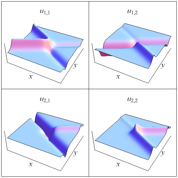
Figure 1: Plot of $u=(u_{i,j})_{2\times 2}$ with $t=0$, $p_{1}=-\frac{1}{4}$, $q_{1}=-\frac{39}{4}$, $p_{2}=\frac{19}{2}$, $q_{2}=\frac{1}{2}$, $r_{1}=2$ and $r_{2}=1$.

3 Quasigrammian solutions of the ncmKP equation

The construction of this particular binary Darboux transformation is given in [18] and also in [17] (for Lax operators with matrix coefficients). The adjoint Lax pair is

$$L_{\scriptscriptstyle\textrm{mKP}}^{{\dagger}} =\partial_{x}^{2}-2w_{x}^{{\dagger}}-2w^{{\dagger}}\partial_{x}+\partial_{y},$$

$$M_{\scriptscriptstyle\textrm{mKP}}^{{\dagger}} =-4\partial_{x}^{3}+12w^{{\dagger}}\partial_{x}^{2}+6(3w^{{\dagger}}_{x}\!-\!{w^{{\dagger}}}^{2}\!\!-\!W^{{\dagger}})\partial_{x}+6(w^{{\dagger}}_{xx}\!-\![w^{{\dagger}}_{x},w^{{\dagger}}]_{+}\!-\!W^{{\dagger}}_{x})-\partial_{t}.$$

For notational convenience, we denote an element of $\ker L_{\scriptscriptstyle\textrm{mKP}}^{{\dagger}}\cap\ker M_{\scriptscriptstyle\textrm{mKP}}^{{\dagger}}$ by $\phi_{x}$. One introduces a potential $\Omega(\phi,\psi)$ satisfying

$$\Omega(\phi,\psi)_{x} =\psi^{{\dagger}}\phi_{x},\quad\Omega(\phi,\psi)_{y}=2\psi^{{\dagger}}w\phi_{x}+\psi^{{\dagger}}\phi_{xx}-\psi^{{\dagger}}_{x}\phi_{x},$$

$$\Omega(\phi,\psi)_{t} =2(-2\psi_{xx}^{{\dagger}}\phi_{x}-2\psi^{{\dagger}}\phi_{xxx}+2\psi_{x}^{{\dagger}}\phi_{xx}-3\psi^{{\dagger}}w^{2}\phi_{x}-3\psi^{{\dagger}}W\phi_{x}-3\psi^{{\dagger}}w_{x}\phi_{x}$$

$$\qquad+6\psi_{x}^{{\dagger}}w\phi_{x}-6\psi^{{\dagger}}w\phi_{xx}).$$

A binary Darboux transformation is defined by

$$\phi_{[n+1]} =\phi_{[n]}-\theta_{[n]}\Omega(\rho_{[n]},\theta_{[n]})^{-1}\Omega(\rho_{[n]},\phi_{[n]})$$

and

$$\psi_{[n+1]} =\psi_{[n]}-\rho_{[n]}\Omega(\rho_{[n]},\theta_{[n]})^{{\dagger}^{-1}}\Omega(\psi_{[n]},\theta_{[n]})^{{\dagger}},$$

in which

$$\theta_{[n]}=\phi_{[n]}|_{\phi\rightarrow\theta_{n}},\quad\rho_{[n]}=\psi_{[n]}|_{\psi\rightarrow\rho_{n}}.$$

Using the notation $\Theta=(\theta_{1},\ldots\theta_{n})$ and $\mathrm{P}=(\rho_{1},\ldots,\rho_{n})$, we have, for $n\geq 1$

$$\phi_{[n+1]} =\begin{vmatrix}\Omega(\Theta,\mathrm{P})&\Omega(\phi,\mathrm{P})\\ \Theta&\framebox{$\phi$}\end{vmatrix},\quad\psi_{[n+1]}=\begin{vmatrix}\Omega(\Theta,\mathrm{P})^{{\dagger}}&\Omega(\Theta,\psi)^{{\dagger}}\\ \mathrm{P}&\framebox{$\psi$}\end{vmatrix}.$$

The effect of the binary Darboux transformation

$$\widehat{L}_{\scriptscriptstyle\textrm{mKP}}=G_{\theta,\phi_{x}}L_{\scriptscriptstyle\textrm{mKP}}G_{\theta,\phi_{x}}^{-1},\quad\widehat{M}_{\scriptscriptstyle\textrm{mKP}}=G_{\theta,\phi_{x}}M_{\scriptscriptstyle\textrm{mKP}}G_{\theta,\phi_{x}}^{-1}$$

is that

$$\hat{f} =\begin{vmatrix}\Omega&\rho^{{\dagger}}\\ \theta&\framebox{$1$}\end{vmatrix}f,$$

where $f$ is given in (8). After $n$ Darboux transformations we have

$$f_{[n+1]} =\begin{vmatrix}\Omega(\mathrm{P},\Theta)&\mathrm{P}^{{\dagger}}\\ \Theta&\framebox{$I$}\end{vmatrix}f.$$

3.1 Two-soliton matrix solution

The trivial vacuum solution $f=I$ (giving $w=W=\textrm{O}$) gives

$$F =\begin{vmatrix}\Omega(\mathrm{P},\Theta)&\mathrm{P}^{{\dagger}}\\ \Theta&\framebox{$I$}\end{vmatrix}.$$ (23)

The eigenfunctions $\theta_{i}$ and the adjoint eigenfunctions $\rho_{i}$ satisfy (15) and (16) respectively. We again choose the eigenfunction solutions of the form (17). With this, we have

$$\Omega(\theta_{j},\rho_{i}) =\delta_{i,j}I-\frac{p_{j}B_{i}^{T}A_{j}}{q_{i}(p_{j}-q_{i})}e^{(\eta_{j}-\gamma_{i})}.$$

As in the previous section, we take $A_{j}=r_{j}P_{j}$ and $B_{i}=I$. So the solutions $w$ and $W$ will be $d\times d$ matrices.

In the case $n=1$, we obtain a one-soliton matrix solution. Expanding (23) gives

$$F =I+\frac{\frac{r}{q}P}{e^{(\gamma-\eta)}-\frac{rp}{q(p-q)}}.$$

If $r>0$ and either $q>p>0$ or $0>q>p$, or alternatively, if $r<0$ and either $p>q>0$ or $0>p>q$ then

$$w =-F_{x}F^{-1}=-\frac{1}{4}(pq)^{-\frac{1}{2}}(p-q)^{2}P\operatorname{sech}\left(\frac{1}{2}\left(\eta-\gamma+\varphi\right)\right)\operatorname{sech}\left(\frac{1}{2}\left(\eta-\gamma+\chi\right)\right),$$

$$W =-F_{y}F^{-1}=(p+q)w,$$

where $\varphi=\log(\frac{-pr}{q(p-q)})$ and $\chi=\log(\frac{-r}{(p-q)})$. Both $w$ and $W$ have a unique maximum where

$$\eta-\gamma =-\log\left(\frac{-(pq^{-1})^{\frac{1}{2}}r}{(p-q)}\right)=\lambda.$$

In the case $n=d=2$, we obtain a two-soliton $2\times 2$ matrix solution. Expanding (23) gives

$$F =I+\begin{pmatrix}A_{1}e^{\eta_{1}}&A_{2}e^{\eta_{2}}\end{pmatrix}\begin{pmatrix}\delta_{i,j}I-\frac{p_{j}A_{j}}{q_{i}(p_{j}-q_{i})}e^{(\eta_{j}-\gamma_{i})}\end{pmatrix}_{2\times 2}^{-1}\begin{pmatrix}I\frac{e^{-\gamma_{1}}}{q_{1}}\\ I\frac{e^{-\gamma_{2}}}{q_{2}}\end{pmatrix}$$

$$=I+\begin{pmatrix}L_{1}e^{\gamma_{1}}&L_{2}e^{\gamma_{2}}\end{pmatrix}\begin{pmatrix}I\frac{e^{-\gamma_{1}}}{q_{1}}\\ I\frac{e^{-\gamma_{2}}}{q_{2}}\end{pmatrix}=I+\frac{1}{q_{1}}L_{1}+\frac{1}{q_{2}}L_{2}.$$

Solving for $L_{1}$ and $L_{2}$ gives

$$L_{1} =\frac{(p_{2}-q_{1})q_{1}}{h}((p_{1}-q_{2})q_{2}h_{2}I+p_{1}A_{2})A_{1},$$

$$L_{2} =\frac{(p_{1}-q_{2})q_{2}}{h}((p_{2}-q_{1})q_{1}h_{1}I+p_{2}A_{1})A_{2},$$

where $h_{i}=e^{(\gamma_{i}-\eta_{i})}-\frac{p_{i}r_{i}}{(p_{i}-q_{i})q_{i}}$, $h=h_{1}h_{2}q_{1}q_{2}(p_{1}-q_{2})(p_{2}-q_{1})-\alpha p_{1}p_{2}r_{1}r_{2}$ and $\alpha$ is as defined in the previous section.

We now investigate the behaviour of $F$ as $t\rightarrow\pm\infty$. We first fix $\eta_{1}-\gamma_{1}$ and assume without loss of generality that $0>p_{2}>q_{2}>p_{1}>q_{1}$. Then, as $t\rightarrow-\infty$,

$$F \sim I+\frac{\frac{r_{1}}{q_{1}}P_{1}}{h_{1}}$$

and therefore

$$w=-F_{x}F^{-1} \sim-\frac{1}{4}(p_{1}q_{1})^{-\frac{1}{2}}(p_{1}-q_{1})^{2}P_{1}\operatorname{sech}\left(\frac{1}{2}\left(\eta_{1}-\gamma_{1}+\varphi_{1}^{-}\right)\right)$$

$$\qquad\times\operatorname{sech}\left(\frac{1}{2}\left(\eta_{1}-\gamma_{1}+\chi_{1}^{-}\right)\right),$$ (24)

where $\varphi_{1}^{-}=\log(\frac{-p_{1}r_{1}}{q_{1}(p_{1}-q_{1})})$ and $\chi_{1}^{-}=\log(\frac{-r_{1}}{(p_{1}-q_{1})})$.

Note that $w=-F_{x}F^{-1}$ and $W=-F_{y}F^{-1}$ are invariant under the transformation $F\rightarrow FC$ where $C$ is a non-singular constant matrix. As $t\rightarrow+\infty$, we get

$$F \!\sim\!I\!+\!\frac{(r_{2}p_{2}(p_{1}\!-\!q_{2})\!-\!p_{1}(p_{2}\!-\!q_{2})A_{2})(p_{2}\!-\!q_{1})A_{1}\!-(p_{2}(p_{1}\!-\!q_{2})A_{1}\!-\!\alpha p_{1}r_{1}(p_{2}\!-\!q_{2}))}{h_{1}r_{2}p_{2}q_{1}(p_{1}\!-\!q_{2})(p_{2}\!-\!q_{1})+\alpha p_{1}p_{2}r_{1}r_{2}(p_{2}\!-\!q_{2})}$$

$$\quad\times(p_{2}\!-\!q_{2})A_{2}\left(I+\frac{(p_{2}-q_{2})A_{2}}{q_{2}r_{2}}\right)$$

$$\sim I+\frac{\frac{\tilde{r}_{1}}{q_{1}}\widetilde{P}_{1}}{e^{\gamma_{1}-\eta_{1}}-\frac{p_{1}\tilde{r}_{1}}{q_{1}(p_{1}-q_{1})}},$$

where $\tilde{r}_{1}=r_{1}\left(1-\frac{\alpha(p_{1}-q_{1})(p_{2}-q_{2})}{(p_{1}-q_{2})(p_{2}-q_{1})}\right)=\frac{r_{1}(\tilde{\mu}_{1},\tilde{\nu}_{1})}{(\mu_{1},\nu_{1})}$, $\tilde{\mu}_{1}=\mu_{1}-\frac{p_{1}(p_{2}-q_{2})(\mu_{1},\nu_{2})\mu_{2}}{p_{2}(p_{1}-q_{2})(\mu_{2},\nu_{2})}$, $\tilde{\nu}_{1}=\nu_{1}-\frac{q_{1}(p_{2}-q_{2})(\mu_{2},\nu_{1})\nu_{2}}{q_{2}(p_{2}-q_{1})(\mu_{2},\nu_{2})}$ and $\widetilde{P}_{1}=\frac{\tilde{\mu}_{1}\otimes\tilde{\nu}_{1}}{(\tilde{\mu}_{1},\tilde{\nu}_{1})}$. Therefore

$$w=-F_{x}F^{-1} \sim-\frac{1}{4}(p_{1}q_{1})^{-\frac{1}{2}}(p_{1}-q_{1})^{2}\widetilde{P}_{1}\operatorname{sech}\left(\frac{1}{2}\left(\eta_{1}-\gamma_{1}+\varphi_{1}^{+}\right)\right)$$

$$\qquad\times\operatorname{sech}\left(\frac{1}{2}\left(\eta_{1}-\gamma_{1}+\chi_{1}^{+}\right)\right),$$ (25)

where $\varphi_{1}^{+}=\log(\frac{-p_{1}\tilde{r}_{1}}{q_{1}(p_{1}-q_{1})})$ and $\chi_{1}^{+}=\log(\frac{-\tilde{r}_{1}}{(p_{1}-q_{1})})$.

Similarly, fixing $\gamma_{2}-\eta_{2}$ gives

$$w \sim-\frac{1}{4}(p_{2}q_{2})^{-\frac{1}{2}}(p_{2}-q_{2})^{2}\widetilde{P}_{2}\operatorname{sech}\left(\frac{1}{2}\left(\eta_{2}-\gamma_{2}+\varphi_{2}^{-}\right)\right)$$

$$\qquad\times\operatorname{sech}\left(\frac{1}{2}\left(\eta_{2}-\gamma_{2}+\chi_{2}^{-}\right)\right),\quad t\rightarrow-\infty,$$ (26)

$$w \sim-\frac{1}{4}(p_{2}q_{2})^{-\frac{1}{2}}(p_{2}-q_{2})^{2}P_{2}\operatorname{sech}\left(\frac{1}{2}\left(\eta_{2}-\gamma_{2}+\varphi_{2}^{+}\right)\right)$$

$$\qquad\times\operatorname{sech}\left(\frac{1}{2}\left(\eta_{2}-\gamma_{2}+\chi_{2}^{+}\right)\right),\quad t\rightarrow+\infty,$$ (27)

where $\tilde{r}_{2}=r_{2}\left(1-\frac{\alpha(p_{1}-q_{1})(p_{2}-q_{2})}{(p_{1}-q_{2})(p_{2}-q_{1})}\right)=\frac{r_{2}(\tilde{\mu}_{2},\tilde{\nu}_{2})}{(\mu_{2},\nu_{2})}$, $\tilde{\mu}_{2}=\mu_{2}-\frac{p_{2}(p_{1}-q_{1})(\mu_{2},\nu_{1})\mu_{1}}{p_{1}(p_{2}-q_{1})(\mu_{1},\nu_{1})}$, $\tilde{\nu}_{2}=\nu_{2}-\frac{q_{2}(p_{1}-q_{1})(\mu_{1},\nu_{2})\nu_{1}}{q_{1}(p_{1}-q_{2})(\mu_{1},\nu_{1})}$, $\widetilde{P}_{2}=\frac{\tilde{\mu}_{2}\otimes\tilde{\nu}_{2}}{(\tilde{\mu}_{2},\tilde{\nu}_{2})}$, $\varphi_{2}^{-}=\log(\frac{-p_{2}\tilde{r}_{2}}{q_{2}(p_{2}-q_{2})})$, $\chi_{2}^{-}=\log(\frac{-\tilde{r}_{2}}{(p_{2}-q_{2})})$, $\varphi_{2}^{+}=\log(\frac{-p_{2}r_{2}}{q_{2}(p_{2}-q_{2})})$ and $\varphi_{2}^{-}=\log(\frac{-p_{2}r_{2}}{q_{2}(p_{2}-q_{2})})$.

The soliton phase shifts $\Lambda_{i}=\lambda_{i}^{+}-\lambda_{i}^{-}$ are

$$\Lambda_{1} =\log\left(\frac{r_{1}}{\tilde{r}_{1}}\right)\ =-\log\beta,\quad\Lambda_{2}=\log\left(\frac{\tilde{r}_{2}}{r_{2}}\right)\ =\log\beta.$$

The matrix amplitude of the first soliton changes from
$-\frac{1}{4}(p_{1}q_{1})^{-\frac{1}{2}}(p_{1}-q_{1})^{2}P_{1}$ to $-\frac{1}{4}(p_{1}q_{1})^{-\frac{1}{2}}(p_{1}-q_{1})^{2}\widetilde{P}_{1}$ and the matrix amplitude of the second soliton changes from $-\frac{1}{4}(p_{2}q_{2})^{-\frac{1}{2}}(p_{2}-q_{2})^{2}\widetilde{P}_{2}$ to
$-\frac{1}{4}(p_{2}q_{2})^{-\frac{1}{2}}(p_{2}-q_{2})^{2}P_{2}$ as $t$ changes from $-\infty$ to $+\infty$. Figure 2 shows a plot of the interaction with $P_{1}=\begin{pmatrix}1&-1\\ 0&0\end{pmatrix}$ and $P_{2}=\frac{1}{13}\begin{pmatrix}16&-6\\ 8&-3\end{pmatrix}$.

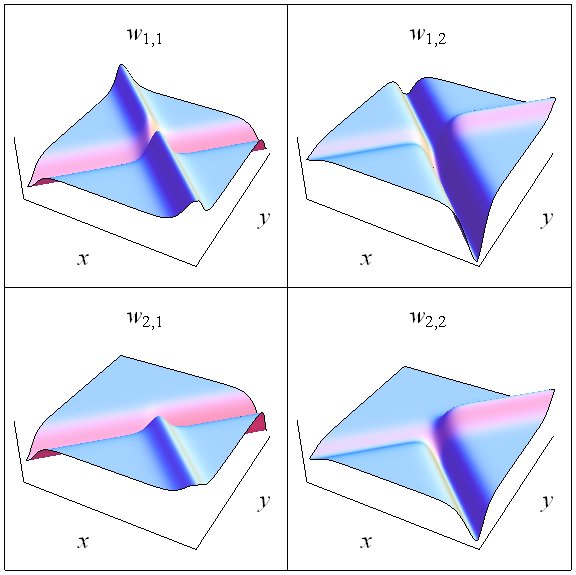
Figure 2: Plot of $w=(w_{i,j})_{2\times 2}$ with $t=0$, $p_{1}=\frac{1}{4}$, $q_{1}=\frac{3}{4}$, $p_{2}=-\frac{1}{4}$, $q_{2}=-\frac{3}{4}$, $r_{1}=1$ and $r_{2}=-1$.

4 Conclusions

In this paper, we have considered a noncommutative KP and a noncommutative mKP equation. It was shown that solutions of ncmKP obtained from a binary Darboux transformation could be expressed as a single quasideterminant. In addition, we have used methods similar to those employed in [8] and obtained matrix versions of both ncKP and ncmKP. Finally, we investigated the interaction properties of the two-soliton solution of both ncKP and ncmKP. This showed that as well as undergoing a phase-shift, the amplitude of each soliton can also change, giving a more elegant picture than the commutative case.

References

[1]
A. Dimakis and F. Müller-Hoissen.
The Korteweg–de-Vries equation on a noncommutative space-time.
Phys. Lett. A, 278(3):139–145, 2000.
[2]
A. Dimakis and F. Müller-Hoissen.
Functional representations of integrable hierarchies.
J. Phys. A, 39(29):9169–9186, 2006.
[3]
A. Dimakis and F. Müller-Hoissen.
Burgers and Kadomtsev-Petviashvili hierarchies: the functional
representation method.
Teoret. Mat. Fiz., 152(1):66–82, 2007.
[4]
I. M. Gelfand, S. Gelfand, V. S. Retakh, and R. L. Wilson.
Quasideterminants.
Adv. Math., 193(1):56–141, 2005.
[5]
C. R. Gilson and J. J. C. Nimmo.
On a direct approach to quasideterminant solutions of a
noncommutative KP equation.
J. Phys. A, 40(14):3839–3850, 2007.
[6]
C. R. Gilson, J. J. C. Nimmo, and C. M. Sooman.
On a direct approach to quasideterminant solutions of a
noncommutative modified KP equation.
J. Phys. A, 41:085202, 2008.
[7]
V. M. Goncharenko.
On the monodromy of matrix Schrödinger equations and the
interaction of matrix solitons.
Uspekhi Mat. Nauk, 55(5(335)):175–176, 2000.
[8]
V. M. Goncharenko.
On multisoliton solutions of the matrix KdV equation.
Teoret. Mat. Fiz., 126(1):102–114, 2001.
[9]
V. M. Goncharenko and A. P. Veselov.
Monodromy of the matrix Schrödinger equations and Darboux
transformations.
J. Phys. A, 31(23):5315–5326, 1998.
[10]
V. M. Goncharenko and A. P. Veselov.
Yang-Baxter maps and matrix solitons.
In New trends in integrability and partial solvability, volume
132 of NATO Sci. Ser. II Math. Phys. Chem., pages 191–197. Kluwer
Acad. Publ., Dordrecht, 2004.
[11]
Masashi Hamanaka.
Noncommutative solitons and integrable systems.
In Noncommutative geometry and physics, pages 175–198. World
Sci. Publ., Hackensack, NJ, 2005.
[12]
Masashi Hamanaka and Kouichi Toda.
Noncommutative Burgers equation.
J. Phys. A, 36(48):11981–11998, 2003.
[13]
Boris A. Kupershmidt.
KP or mKP, volume 78 of Mathematical Surveys and
Monographs.
American Mathematical Society, Providence, RI, 2000.
Noncommutative mathematics of Lagrangian, Hamiltonian, and integrable
systems.
[14]
Olaf Lechtenfeld, Liuba Mazzanti, Silvia Penati, Alexander D. Popov, and Laura
Tamassia.
Integrable noncommutative sine-Gordon model.
Nuclear Phys. B, 705(3):477–503, 2005.
[15]
C. X. Li and J. J. C. Nimmo.
Quasideterminant solutions of a non-abelian Toda lattice and kink
solutions of a matrix sine-Gordon equation.
Proc. R. Soc. Lond. Ser. A Math. Phys. Eng. Sci.,
464(2092):951–966, 2008.
[16]
V. B. Matveev and M. A. Salle.
Darboux transformations and solitons.
Springer Series in Nonlinear Dynamics. Springer-Verlag, Berlin, 1991.
[17]
J. J. C. Nimmo.
Darboux transformations from reductions of the KP hierarchy.
In Nonlinear evolution equations & dynamical systems: NEEDS
’94 (Los Alamos, NM), pages 168–177. World Sci. Publ., River Edge,
NJ, 1995.
[18]
W. Oevel and C. Rogers.
Gauge transformations and reciprocal links in dimensions.
Rev. Math. Phys., 5(2):299–330, 1993.
[19]
Ning Wang and Miki Wadati.
Noncommutative KP hierarchy and Hirota triple-product relations.
J. Phys. Soc. Japan, 73(7):1689–1698, 2004.