Calculation of Anderson localization criterium for a one dimensional chain with diagonal disorder

Abstract

For a one dimensional half-infinite chain with diagonal disorder we calculated the ultimate at $t\rightarrow\infty$ value of the average excitation density at the edge site $D$ if at $t=0$ the excitation was localised at the edge site (Anderson’ s creterium). We obtained the following results: i) for the binary disordered chain we derived the close expression for $D$ which is exact in the limit of low concentration of defects and is valid for an arbitrary energy of defects $\varepsilon$. In this case $D$ demonstrated the non analytical dependence on $\varepsilon$. ii) The close expression for $D$ is obtained for the case of an arbitrary small disorder. iii) The relative contribution of states with specified energy to $D$ is calculated. All the results obtained are in complete agreement with computer simulation.

I Introduction, the problem setting, and main results

The mathematical models of contemporary physics of disordered systems can be divided into two classes – continuous and discrete. The continuous models are those in which the Shredinger equation $(-\Delta+v(r))\psi=E\psi$ with random potential $v(r)$ is studied while the discrete models are dealing with the random matrix of Hamiltonian. These two types of models have much in common but despite the similarity they may require essentially different methods of analysis due to the following reason. It is well known Lif that the possibility of the localized states whose wave functions are essentially differes from zero within the finite region when the system volume runs to infinity is one of the most important properties of the homogeneous disordered systems. For the continuous models of infinite volume the localized states can be recognized by dividing the energy spectrum into discrete and continuous parts with square integrated states of the discrete part considered to be localized. The energy spectrum of discrete models being the spectrum of random matrix is always discrete and for this reason one should use another criterium for states characterization in this case. The Anderson criterium is one of the relevant onesAnd ; Lif .

The deep theoretical analysis is possible for the one dimensional models of disordered systems which we have in mind hereafter. It is commonly accepted that the spectrum of one dimensional Shredinger equation with random potential is completely discrete what is correspond to localization of all states for an arbitrary low disorder Lif . The validity of this statement to the discrete models is arguable because of completely discrete character of spectrum of such models even in the absence of disorder when all states are delocalized. In present paper we study the character of states in the sense of Anderson criterium for the case of one dimensional chain (discrete model) with diagonal disorder. The simple physical sense of this criterium allows one to apply it both to discrete and continuous models.

Let’s turn to the problem setting and consider the one dimensional diagonally disordered discrete model with the Hamiltonian whose matrix has the following entries:

$$H_{r,r^{\prime}}=\delta_{r,r^{\prime}}\varepsilon_{r}+\delta_{r,r^{\prime}+1}+\delta_{r,r^{\prime}-1},\hskip 28.45274ptr,r^{\prime}=1,...,N$$ (1)

Such Hamiltonian describe the Frenkel exciton in the chain consisting of N two-level atoms in the nearest neighbour approximation. In this model the level splitting $\varepsilon_{r}$ of r-th atom is considered to be the random variable distributed in accordance with the function $P$ which is supposed known.

The unit non diagonal elements of Eq.(1) are specify the scale of energy. Everywhere below the thermodynamic limit $N\rightarrow\infty$ is implied. For this model we now set the following problem. Let us suppose that the edge atom was prepared in the excited state at $t=0$ and one should calculate the probability $D$ for this atom to remain in the excited state at $t\rightarrow\infty$. From the mathematical point of view it means that the initial state of the system is described by the wavefunction (column-vector) ${\bf\Psi}(0)$ with entries $\Psi_{r}(0)=\delta_{r,N}$ and one should find $D=\langle|\Psi_{N}(t\rightarrow\infty)|^{2}\rangle$ where angular brackets denote the averaging over the random level splittings $\varepsilon_{r}$. The temporary dependance of the wavefunction can be written as: ${\bf\Psi}(t)=\exp\bigg{(}\imath{\bf H}t\bigg{)}{\bf\Psi}(0)$. Consequently the quantity of interest $D$ can be expressed in terms of eigen vectors ${\bf\Psi}^{\lambda}$ and eigen numbers $E_{\lambda},\lambda=1,...,N$ of the matrix Eq.(1) as:

$$D=\langle|\Psi_{N}(t\rightarrow\infty)|^{2}\rangle=\lim_{t\rightarrow\infty}\bigg{\langle}\sum_{\lambda\lambda^{\prime}}|\Psi^{\lambda}_{N}|^{2}|\Psi^{\lambda^{\prime}}_{N}|^{2}\exp\imath(E_{\lambda}-E_{\lambda^{\prime}})t\bigg{\rangle}=\bigg{\langle}\sum_{\lambda}|\Psi^{\lambda}_{N}|^{4}\bigg{\rangle}$$ (2)

The similar quantities were analysed in the numerical study of disordered chains for instance in Mal . Regarding $D$ one can make the following qualitative conclusions. Suppose all the eigen functions of Hamiltonian Eq.(1) are delocalized in the sense of their amplitude being nearly the same within an arbitrary region of the chain. The amplitude squared of such functions at the edge site can be estimated as $|\Psi_{N}^{\lambda}|^{2}\sim 1/N$ with all $N$ eigen functions giving nearly the same contribution $|\Psi_{N}^{\lambda}|^{4}\sim 1/N^{2}$ to Eq.(2). Consequently, if the states of Eq.(1) are delocalized in the above sense then in the thermodynamic limit $D\sim 1/N\rightarrow 0$. Let’s consider now the situation when some of the eigen functions of Eq.(1) are localized in the sense of their amplitude being essentially non-zero only in some restricted region of the chain with the size of this region being independent on $N$ when $N\rightarrow\infty$. Being defined only by the functions whose amplitude is essentially non-zero at the edge site the contribution of functions of this type to Eq.(2) will not depend on $N$. In this case $D$ remain finite in the thermodynamic limit. Having in mind all above qualitative conclusions one can introduce Anderson’s criterium as: If $D$ is remain finite in the thermodynamic limit then in the set of eigen functions of Hamiltonian Eq.(1) there exist ones localized in the sense of Anderson’s criterium.

To get some information concerning the degree of localization of eigen vectors of Eq.(1) in some (specified) spectral range we now introduce the ”participation” function defined as:

$$W(U)dU=\bigg{\langle}\sum_{E_{\lambda}\in[U,U+dU]}|\Psi^{\lambda}_{N}|^{4}\bigg{\rangle},$$ (3)

Obviously $D=\int W(U)dU$. Reasoning analogous to that presented above shows that if all the states within the interval $[U,U+dU]$ are delocalized then $W(U)=0$. In the opposite case $W(U)$ differs from zero. Moreover, the function (3) provide quantitative information concerning the average value of eigen vectors of random matrix Eq.(1) at the edge site within the spectral interval $[U,U+dU]$. The fantastic capabilities of modern personal computers allows one to perform direct diagonalisation of the matrix Eq.(1) for $N\sim 1000$ and more and in such numerical experiment to ”observe” quantities Eq.(2) and Eq.(3). The theoretical calculation of these quantities is the main goal of this paper.

The main results obtained in the present paper are:

1. The perturbation theory for calculation of joint distribution function of advanced and retarded Green’s functions of Hamiltonian Eq.(1) is developed.

2. For the binary disordered one dimensional system, described by Hamiltonian (1) with the atomic splittings $\varepsilon_{r}$ being equal to zero with probability $1-c$ and equal to $\varepsilon$ with probability $c$ ($0<c<1$) the following expressions for $D$ and $W(U)$ function are obtained:

$$D={c\over 4\pi}\int_{-2}^{2}dU(4-U^{2})^{3/2}\hskip 2.84526pt\hbox{ln}\bigg{(}{\varepsilon^{2}\over 4-U^{2}}+1\bigg{)}+c\hskip 2.84526pt\Theta(|\varepsilon|-1)\bigg{(}{\varepsilon^{2}-1\over\varepsilon^{2}}\bigg{)}^{2}+O(c^{2})$$ (4)

$$W(U)={c\over 4\pi}\Theta(2-|U|)(4-U^{2})^{3/2}\hskip 2.84526pt\hbox{ln}\bigg{(}{\varepsilon^{2}\over 4-U^{2}}+1\bigg{)}+$$ (5)

$$+c\Theta(|\varepsilon|-1)\bigg{(}{\varepsilon^{2}-1\over\varepsilon^{2}}\bigg{)}^{2}\delta\bigg{(}U-{\varepsilon^{2}+1\over\varepsilon}\bigg{)}+O(c^{2})$$

Nonanalyticity with respect to $\varepsilon$ is related to the occurrence (when $|\varepsilon|>1$) of the edge state with eigen energy $U_{0}=(\varepsilon^{2}+1)/\varepsilon$.

3. For the wide class of disordered systems described by Hamiltonian (1) with random atomic splittings $\varepsilon_{r}$ having the distribution functions in the form $P_{\Delta}(x)=p(x/\Delta)/\Delta$ (where $p(x)>0,\int p(x)dx=1,\int p(x)xdx=0,\int p(x)x^{2}dx=M_{2}$) the following expressions for $D$ and $W(U)$ function are obtained:

$$D={\Delta^{2}M_{2}\over 2}+O(\Delta^{3}),\hskip 28.45274ptW(U)=\Theta(2-|U|){\Delta^{2}M_{2}\over 4\pi}\sqrt{4-U^{2}}+O(\Delta^{3})$$ (6)

All the results obtained in the paper were verified by the computer simulation which shows that when $D<0.1$ the deviation of formulas Eq.(4 – 6) from the numerical results is less than $10\%$. In this case the degree of disorder may be rather large. For example formula Eq.(6) is still valid when $\varepsilon_{r}$ values are uniformly distributed within the interval $[-0.25,0.25]$.

II Statistics of Green’s functions

It is easy to show that the quantity $\langle|\Psi_{N}(t)|^{2}\rangle$ (with the quantity of interest $D=\langle|\Psi_{N}(\infty)|^{2}\rangle$) can be calculated as:

$$\langle|\Psi_{N}(t)|^{2}\rangle=\lim_{V_{1,2}\rightarrow+0}{1\over 4\pi^{2}}\int dU_{1}dU_{2}\exp[\imath(U_{1}-U_{2})t]\langle\gamma(U_{1}-\imath V_{1})\gamma(U_{2}+\imath V_{2})\rangle$$ (7)

Where $\gamma(\Omega)$ – is the edge Green’s function (EGF) for Hamiltonian Eq.(1):

$$\gamma(\Omega)\equiv\sum_{\lambda}{|\Psi_{N}^{\lambda}|^{2}\over\Omega-E_{\lambda}}$$ (8)

To calculate the mean product of two Green’s functions entering Eq.(7) one should know their joint distribution function. We obtain the equation for this function by generalising the Dyson’s method Dyson ; Lif . Let’s denote by $\gamma(\Omega_{i}),i=1,2$ the edge Green’s functions Eq.(8) with complex energies $\Omega_{1}\equiv U_{1}-\imath V_{1}$ and $\Omega_{2}\equiv U_{2}+\imath V_{2}$ and add one more atom with splitting $\varepsilon$ to the chain. Then as it is shown in Dyson ; Lif EGF of the chain with added atom $\tilde{\gamma}(\Omega)$ can be expressed in terms of EGF of the initial chain as:

$$\tilde{\gamma}(\Omega)={1\over\Omega-\varepsilon-\gamma(\Omega)}$$ (9)

To describe the EGFs of the initial chain $\gamma(\Omega_{i}),i=1,2$ we introduce the distribution function $\eta$ defined in such a way that the quantity $\eta(x_{1},y_{1},x_{2},y_{2})dx_{1}dy_{1}dx_{2}dy_{2}$ gives the probability of Re $\gamma(\Omega_{i})\in[x_{i},x_{i}+dx_{i}]$ and Im $\gamma(\Omega_{i})\in[y_{i},y_{i}+dy_{i}],i=1,2$. We denote by $\tilde{\eta}$ the analagous function for the chain with added atom. The relation Eq.(9) allows one to express $\tilde{\eta}$ in terms of $\eta$ and the distribution function of atomic splittings $P(\varepsilon)$:

$$\tilde{\eta}(\tilde{x_{1}},\tilde{y_{1}},\tilde{x_{2}},\tilde{y_{2}})=\int\delta\bigg{(}\tilde{x_{1}}-\hbox{Re}{1\over\Omega_{1}-\varepsilon-x_{1}-\imath y_{1}}\bigg{)}\delta\bigg{(}\tilde{y_{1}}-\hbox{Im}{1\over\Omega_{1}-\varepsilon-x_{1}-\imath y_{1}}\bigg{)}\times$$ (10)

$$\delta\bigg{(}\tilde{x_{2}}-\hbox{Re}{1\over\Omega_{2}-\varepsilon-x_{2}-\imath y_{2}}\bigg{)}\delta\bigg{(}\tilde{y_{2}}-\hbox{Im}{1\over\Omega_{2}-\varepsilon-x_{2}-\imath y_{2}}\bigg{)}\eta(x_{1}y_{1}x_{2}y_{2})P(\varepsilon)dx_{1}dy_{1}dx_{2}dy_{2}d\varepsilon$$

In the thermodynamic limit $N\rightarrow\infty$ it must be $\eta=\tilde{\eta}$. Calculating the integrals with $\delta$-functions in Eq.(10) we obtain for the steady state function $\eta$ the following equation:

$$(x^{2}_{1}+y^{2}_{1})^{2}(x^{2}_{2}+y^{2}_{2})^{2}\eta(x_{1},y_{1},x_{2},y_{2})=$$ (11)

$$=\int\eta\bigg{(}U_{1}-\varepsilon-{x_{1}\over x^{2}_{1}+y^{2}_{1}},\hskip 5.69054pt-V_{1}+\hskip 2.84526pt{y_{1}\over x^{2}_{1}+y^{2}_{1}},\hskip 5.69054ptU_{2}-\varepsilon-{x_{2}\over x^{2}_{2}+y^{2}_{2}},\hskip 5.69054ptV_{2}+\hskip 2.84526pt{y_{2}\over x^{2}_{2}+y^{2}_{2}}\bigg{)}P(\varepsilon)d\varepsilon$$

Using the function $\eta$ one can introduce the mean product of the advanced and retarded Green’s functions entering Eq.(7) as a sum of four terms:

$$\langle\gamma(\Omega_{1})\gamma(\Omega_{2})\rangle=\int\eta(x_{1}y_{1}x_{2}y_{2})[x_{1}x_{2}-y_{1}y_{2}+\imath(y_{1}x_{2}+y_{2}x_{1})]dx_{1}dx_{2}dy_{1}dy_{2}\equiv$$ (12)

$$=\langle x_{1}x_{2}\rangle-\langle y_{1}y_{2}\rangle+\imath\langle y_{1}x_{2}\rangle+\imath\langle y_{2}x_{1}\rangle$$

Using the expression Eq.(8) it is easy to see that these terms can be written in the representation of Hamiltonian Eq.(1) as:

$$\langle x_{1}x_{2}\rangle=\bigg{\langle}\sum_{\lambda\lambda^{\prime}}{|\Psi_{N}^{\lambda}|^{2}|\Psi_{N}^{\lambda^{\prime}}|^{2}(U_{1}-E_{\lambda})(U_{2}-E_{\lambda^{\prime}})\over[(U_{1}-E_{\lambda})^{2}+V_{1}^{2}][(U_{2}-E_{\lambda^{\prime}})^{2}+V_{2}^{2}]}\bigg{\rangle}$$ (13)

$$-\langle y_{1}y_{2}\rangle=\bigg{\langle}\sum_{\lambda\lambda^{\prime}}{|\Psi_{N}^{\lambda}|^{2}|\Psi_{N}^{\lambda^{\prime}}|^{2}V_{1}V_{2}\over[(U_{1}-E_{\lambda})^{2}+V_{1}^{2}][(U_{2}-E_{\lambda^{\prime}})^{2}+V_{2}^{2}]}\bigg{\rangle}$$

$$\imath\langle y_{1}x_{2}\rangle=\imath\bigg{\langle}\sum_{\lambda\lambda^{\prime}}{|\Psi_{N}^{\lambda}|^{2}|\Psi_{N}^{\lambda^{\prime}}|^{2}V_{1}(U_{2}-E_{\lambda^{\prime}})\over[(U_{1}-E_{\lambda})^{2}+V_{1}^{2}][(U_{2}-E_{\lambda^{\prime}})^{2}+V_{2}^{2}]}\bigg{\rangle}$$

$$\imath\langle x_{1}y_{2}\rangle=-\imath\bigg{\langle}\sum_{\lambda\lambda^{\prime}}{|\Psi_{N}^{\lambda}|^{2}|\Psi_{N}^{\lambda^{\prime}}|^{2}V_{2}(U_{1}-E_{\lambda})\over[(U_{1}-E_{\lambda})^{2}+V_{1}^{2}][(U_{2}-E_{\lambda^{\prime}})^{2}+V_{2}^{2}]}\bigg{\rangle}$$

Thus, $\langle|\Psi_{N}(t)|^{2}\rangle$ Eq.(7) can be represented as a sum of four contributions:

$$\langle|\Psi_{N}(t)|^{2}\rangle=\Delta_{\langle x_{1}x_{2}\rangle}+\Delta_{\langle y_{1}y_{2}\rangle}+\Delta_{\langle y_{1}x_{2}\rangle}+\Delta_{\langle x_{1}y_{2}\rangle}.$$ (14)

We present the calculation of $\Delta_{\langle y_{2}x_{1}\rangle}$ as an example:

$$\Delta_{\langle y_{2}x_{1}\rangle}={\imath\over 4\pi^{2}}\lim_{V_{1,2}\rightarrow+0}\int dU_{1}dU_{2}\exp\imath(U_{1}-U_{2})t\hskip 5.69054pt\langle y_{2}x_{1}\rangle=$$ (15)

$$=-{\imath\over 4\pi^{2}}\lim_{V_{1,2}\rightarrow+0}\int dU_{1}dU_{2}\hskip 5.69054pt\exp\imath(U_{1}-U_{2})t\hskip 5.69054pt\bigg{\langle}\sum_{\lambda\lambda^{\prime}}{|\Psi_{N}^{\lambda}|^{2}|\Psi_{N}^{\lambda^{\prime}}|^{2}V_{2}(U_{1}-E_{\lambda})\over[(U_{1}-E_{\lambda})^{2}+V_{1}^{2}][(U_{2}-E_{\lambda^{\prime}})^{2}+V_{2}^{2}]}\bigg{\rangle}=$$

$$={1\over 4}\bigg{\langle}\sum_{\lambda\lambda^{\prime}}|\Psi_{N}^{\lambda}|^{2}|\Psi_{N}^{\lambda^{\prime}}|^{2}\exp\imath(E_{\lambda}-E_{\lambda^{\prime}})t\bigg{\rangle}$$

The similar calculations shows that all four contributions Eq.(14) to $\langle|\Psi_{N}(t)|^{2}\rangle$ are equal to each other: $\Delta_{\langle x_{1}x_{2}\rangle}=\Delta_{\langle y_{1}y_{2}\rangle}=\Delta_{\langle y_{1}x_{2}\rangle}=\Delta_{\langle x_{1}y_{2}\rangle}$ and therefore:

$$\langle|\Psi_{N}(t)|^{2}\rangle=4\Delta_{\langle y_{2}x_{1}\rangle}$$ (16)

The following remark is important for what is hearafter. Suppose that the integration over $U_{1,2}$ in Eq.(15) runs over the small region $U_{1,2}\in[U,U+dU]$ only and we are interested in the behaviour of $\Delta_{\langle y_{2}x_{1}\rangle}$ contribution at $t\rightarrow\infty$. In this case the sum in the last string of Eq.(15) will contain the states with energies $E_{\lambda}\in[U,U+dU]$ only. So, it is seen that such restriction of the integration region allows one to calculate the ”participation” function Eq.(3).

Thus, the problem reduced to solving of the Eq.(11) for the joint probability distribution function $\eta$. The fact that when calculating the contributions Eq.(13) the limit $V_{1,2}\rightarrow+0$ is implied one can use for reducing the problem to studying the equation which is much easier than Eq.(11). To do this we note that if $V_{1}=V_{2}=0$ then the solution of Eq.(11) can be presented in the form:

$$\eta(x_{1},y_{1},x_{2},y_{2})\bigg{|}_{V_{1,2}=0}=\delta(y_{1})\delta(y_{2})\rho(x_{1},x_{2}),$$ (17)

where the depending on $U_{1,2}$ function $\rho(x_{1},x_{2})$ satisfy the following equation:

$$x_{1}^{2}x_{2}^{2}\rho(x_{1},x_{2})=\int P(\varepsilon)\rho(U_{1}-\varepsilon-1/x_{1},\hskip 5.69054ptU_{2}-\varepsilon-1/x_{2})d\varepsilon$$ (18)

Now let us perform the calculation of the quantity $\langle y_{2}x_{1}\rangle$ taking into account that for small $V_{1,2}$ the solution of Eq.(11) goes to Eq.(17). Using the fact that the function $\eta$ is satisfy to Eq.(11) one can write the following expression for the mean of interest $\langle y_{2}x_{1}\rangle$:

$$\langle y_{2}x_{1}\rangle=\int\eta(x_{1}y_{1}x_{2}y_{2})y_{2}x_{1}dx_{1}dx_{2}dy_{1}dy_{2}=$$ (19)

$$\int{dx_{1}dx_{2}dy_{1}dy_{2}d\varepsilon\hskip 1.42262pty_{2}x_{1}\over(x_{1}^{2}+y_{1}^{2})^{2}(x_{2}^{2}+y_{2}^{2})^{2}}\eta\bigg{(}U_{1}-\varepsilon-{x_{1}\over x_{1}^{2}+y_{1}^{2}},-V_{1}+{y_{1}\over x_{1}^{2}+y_{1}^{2}},U_{2}-\varepsilon-{x_{2}\over x_{2}^{2}+y_{2}^{2}},V_{2}+{y_{2}\over x_{2}^{2}+y_{2}^{2}}\bigg{)}P(\varepsilon)=$$

By replacing the variables:

$$-{x_{k}\over y_{k}^{2}+x_{k}^{2}}\rightarrow x_{k},\hskip 28.45274pt{y_{k}\over y_{k}^{2}+x_{k}^{2}}\rightarrow y_{k}\hskip 28.45274ptk=1,2$$ (20)

and calculating the corresponding Jacobians one can continue the equality Eq.(19) as:

$$=-\int dx_{1}dx_{2}dy_{1}dy_{2}d\varepsilon\hskip 5.69054pt\eta(U_{1}-\varepsilon+x_{1},y_{1}-V_{1},U_{2}-\varepsilon+x_{2},V_{2}+y_{2}){x_{1}\over y_{1}^{2}+x_{1}^{2}}{y_{2}\over y_{2}^{2}+x_{2}^{2}}$$

Taking advantage of the fact that when $V_{1,2}\rightarrow+0$ the function $\eta$ is close to Eq.(17) one can conclude that in the region where the expression under this integral is essentially differs from zero the following estimations are valid: $y_{1}\approx V_{1},y_{2}\approx-V_{2}$, with the accuracy of estimations increasing in the limit $V_{1,2}\rightarrow+0$. In this limit $y_{2}/(y_{2}^{2}+x_{2}^{2})\rightarrow-\pi\delta(x_{2})$, and $y_{1}\rightarrow+0$. Having all this in mind one can now perform the integration over $x_{2}$, replace the function $\eta$ by its ultimate expression Eq.(17) and finally get:

$$\langle y_{2}x_{1}\rangle=\pi\int d\varepsilon{dx\over x}\hskip 5.69054pt\rho(U_{1}-\varepsilon+x,U_{2}-\varepsilon)P(\varepsilon),$$ (21)

Here we imply the main value of the integral. The same calculations can be performed for $\langle y_{1}x_{2}\rangle$, $\langle y_{1}y_{2}\rangle$ and $\langle x_{1}x_{2}\rangle$.

In the end one should take into account the following important remark. It is seen from the Eq.(15) that if $\langle y_{2}x_{1}\rangle$ has no singularity at $U_{2}-U_{1}\equiv\omega=0$ then $\lim_{t\rightarrow\infty}\Delta_{\langle y_{2}x_{1}\rangle}=0$. Therefore the non-zero value of $D$ is related to the occuarence of the singularity of $\langle y_{2}x_{1}\rangle$ at $\omega=0$. Thus, for calculation of $D$ it is sufficient to solve the Eq.(18) for small $\omega$, extract the singular part and use it for the calculation of ultimate at $t\rightarrow\infty$ behaviour of the integral in Eq.(15). This will be done in the next sections

III Binary disorder

In the case of binary disorder mentioned in the first section the distribution function of atomic levels splittings has the form:

$$P(y)=(1-c)\delta(y)+c\delta(y-\varepsilon),\hskip 28.45274pt0<c<1$$ (22)

and Eq.(18) can be written as:

$$x_{1}^{2}x_{2}^{2}\rho(x_{1}x_{2})=(1-c)\rho(U_{1}-1/x_{1},U_{2}-1/x_{2})+c\rho(U_{1}-\varepsilon-1/x_{1},U_{2}-\varepsilon-1/x_{2})$$ (23)

We now introduce the function $\rho$ as a series in powers of $c$:

$$\rho=\sum_{n=0}^{\infty}c^{n}\rho_{n}$$ (24)

By substituting this series into Eq.(23) and equating the coefficients at equal powers of $c$ one can obtain:

$$c^{0}:\hskip 28.45274pt\rho_{0}(x_{1}x_{2})x_{1}^{2}x_{2}^{2}=\rho_{0}(U_{1}-1/x_{1},U_{2}-1/x_{2})$$ (25)

$$\hskip 8.53581ptc^{1}:\hskip 28.45274pt\rho_{1}(x_{1}x_{2})x_{1}^{2}x_{2}^{2}=\rho_{1}(U_{1}-1/x_{1},U_{2}-1/x_{2})+$$ (26)

$$+\rho_{0}(U_{1}-\varepsilon-1/x_{1},U_{2}-\varepsilon-1/x_{2})-\rho_{0}(U_{1}-1/x_{1},U_{2}-1/x_{2}),\hskip 8.53581pt\hbox{and so on}$$

To calculate the value of $D$ up to the terms of $\sim c^{2}$ it is sufficient to calculate the mean Eq.(21) with the same accuracy. By substituting Eq.(22) and Eq.(24) to Eq.(21) we obtain:

$$\langle y_{2}x_{1}\rangle=\pi\int{dx\over x}\bigg{\{}(1-c)\rho_{0}(U_{1}+x,U_{2})+c\rho_{0}(U_{1}-\varepsilon+x,U_{2}-\varepsilon)+c\rho_{1}(U_{1}+x,U_{2})\bigg{\}}+O(c^{2})$$ (27)

The first term in braces gives the mean $\langle y_{2}x_{1}\rangle$ (up to the factor $1-c$) for the completely ordered chain (when $D=0$) and is not of interest for us. Thus, for the singular part of $\langle y_{2}x_{1}\rangle$ (we denote it as ”sing”) which we are interested in and for the ultimate at $t\rightarrow\infty$ value of $\Delta_{\langle y_{2}x_{1}\rangle}$ we obtain the following expressions:

$$\hbox{sing}\langle y_{2}x_{1}\rangle=c\pi\int{dx\over x}\bigg{\{}\rho_{0}(U_{1}-\varepsilon+x,U_{2}-\varepsilon)+\rho_{1}(U_{1}+x,U_{2})\bigg{\}}+O(c^{2})$$ (28)

$$\lim_{t\rightarrow\infty}\Delta_{\langle y_{2}x_{1}\rangle}={\imath\over 4\pi^{2}}\lim_{t\rightarrow\infty}\int dU_{1}dU_{2}\exp\imath(U_{1}-U_{2})t\hskip 5.69054pt\hbox{sing}\langle y_{2}x_{1}\rangle$$

To obtain the functions $\rho_{0}$ and $\rho_{1}$ entering Eq.(28) one should solve the equations Eq.(25) and Eq.(26). We start the analysis of these equations from the most important case when $|U_{1,2}|<2$, i.e. when energies of both Green’s functions are belong to the spectrum of bare Hamiltonian Eq.(1) at $\varepsilon_{r}=0$.

III.1 The contribution of region $|U_{1,2}|<2$

By direct substitution one can see that in this case the exact solution of Eq.(25) can be written in the close form:

$$\rho_{0}(x_{1}x_{2})={\cal L}_{U_{1}}(x_{1}){\cal L}_{U_{2}}(x_{2}),$$ (29)

where ${\cal L}_{U}(x)$ is Lorentzian:

$${\cal L}_{U}(x)={\sqrt{4-U^{2}}\over 2\pi}{1\over x^{2}-Ux+1}$$ (30)

Let us turn now to the Eq.(26) whose solution for $|U_{1,2}|<2$ we will construct using the system of special functions proposed by the author in Koz . Below we briefly review the results obtained in Koz .

Define the depending on parameter $U,|U|<2$ linear operator ${\cal H}_{U}$ which acts on an arbitrary function in accordance with the following definition:

$${\cal H}_{U}f(x)\equiv{1\over x^{2}}f(U-1/x)$$ (31)

As it is shown in Koz the eigen functions $\sigma^{(n)}_{U}(x)$ and eigen numbers $\lambda_{n}$ (they can be numbered by integer $n$) are defined by the following relations:

$$\sigma_{U}^{(n)}(x)={\cal L}_{U}(x)\bigg{[}{R^{\ast}-x\over R-x}\bigg{]}^{n}\equiv{\cal L}_{U}(x)G^{n}(x),\hskip 8.53581pt\lambda_{n}=\bigg{(}{U+\imath\sqrt{4-U^{2}}\over U-\imath\sqrt{4-U^{2}}}\bigg{)}^{n},\hskip 8.53581pt|\lambda_{n}|=1$$ (32)

where

$$R={U+\imath\sqrt{4-U^{2}}\over 2},\hskip 28.45274ptR^{\ast}={U-\imath\sqrt{4-U^{2}}\over 2},\hskip 14.22636ptRR^{\ast}=1$$

The map corresponding to operator ${\cal H}_{U}$ plays an important role in Eqs. (25), (26) and for this reason we will search for the solution of these equations in the form of the expansion into a set of functions Eq.(32). To do this we use the rules of expansion of an arbitrary function $f(x)$ in a set of functions Eq.(32) obtained in Koz :

$$f(x)=\sum_{n=-\infty}^{+\infty}A_{n}\sigma^{(n)}_{U}(x)$$ (33)

with coefficients $A_{n}$ being defined by formulas:

$$A_{n}=\int{f(x)\over G^{n}(x)}dx$$ (34)

Using the functions Eq.(32) one can expand $\rho_{1}(x_{1}x_{2})$ in series:

$$\rho_{1}(x_{1}x_{2})=\sum_{|n|+|m|\neq 0}C_{nm}\sigma_{U_{1}}^{(n)}(x_{1})\sigma_{U_{2}}^{(m)}(x_{2})$$ (35)

Substituting the series Eq.(35) into Eq.(26) and making use of the properties of functions Eq.(32) one can obtain:

$$\sum_{|n|+|m|\neq 0}C_{nm}\sigma^{(n)}_{U_{1}}(x_{1})\sigma^{(m)}_{U_{2}}(x_{2})[1-\lambda_{n}(U_{1})\lambda_{m}(U_{2})]=$$ (36)

$$={\rho_{0}(U_{1}-\varepsilon-1/x_{1},U_{2}-\varepsilon-1/x_{2})\over x_{1}^{2}x_{2}^{2}}-{\cal L}_{U_{1}}(x_{1}){\cal L}_{U_{2}}(x_{2})$$

With the help of Eq.(33) and Eq.(34) one can expand the r.h.p. of this equation in a set of functions Eq.(32) and obtain the following expressions for the expansion coefficients of $\rho_{1}$:

$$C_{nm}={J_{n}(U_{1},\varepsilon)J_{m}(U_{2},\varepsilon)\over 1-\lambda_{n}(U_{1})\lambda_{m}(U_{2})}$$ (37)

where functions $J_{n}(U,\varepsilon)$ are defined as:

$$J_{n}(U,\varepsilon)\equiv\int{{\cal L}_{U}(U-\varepsilon-1/x)\over G^{n}(x)}{dx\over x^{2}}=\lambda_{n}(U)\int{{\cal L}_{U}(x-\varepsilon)\over G^{n}(x)}dx,$$ (38)

The following (based on the properties of $\sigma^{(n)}_{U}(x)$ functions) relations are take place:

$$J_{n}(U,0)=0\hskip 14.22636pt\hbox{for}\hskip 5.69054ptn\neq 0,\hskip 14.22636ptJ_{n}(U,\varepsilon)=J_{-n}^{\ast}(U,\varepsilon)\Rightarrow|J_{n}(U,\varepsilon)|^{2}=|J_{-n}^{\ast}(U,\varepsilon)|^{2}$$ (39)

Thus, the solution of Eq.(26) for $\rho_{1}$ has the form:

$$\rho_{1}(x_{1}x_{2})=\sum_{|n|+|m|\neq 0}{J_{n}(U_{1},\varepsilon)J_{m}(U_{2},\varepsilon)\over 1-\lambda_{n}(U_{1})\lambda_{m}(U_{2})}\sigma_{U_{1}}^{(n)}(x_{1})\sigma_{U_{2}}^{(m)}(x_{2})$$ (40)

As it was mentioned above only singular at $\omega=U_{2}-U_{1}\approx 0$ part of this expression is needed for calculation of $D$. It easy to see that only terms with $m=-n$ of sum Eq.(40) possess the required peculiarity at $\omega=0$. Now we make the following replacing of symbols: $U_{1}\rightarrow U,U_{2}\rightarrow U+\omega$ and write down the expression for the denominators of these terms up to $\omega^{2}$:

$$1-\lambda_{n}(U)\lambda_{-n}(U+\omega)=-{2\imath n\omega\over\sqrt{4-U^{2}}}+O(\omega^{2})$$ (41)

Taking this into account we obtain the following expression for the singular part of Eq.(40):

$$\hbox{sing}\hskip 2.84526pt\rho_{1}(x_{1}x_{2})={\imath\sqrt{4-U^{2}}\over 2\omega}\sum_{n\neq 0}{|J_{n}(U,\varepsilon)|^{2}\over n}\sigma_{U}^{(n)}(x_{1})\sigma_{U}^{-n}(x_{2})$$ (42)

Let us turn now to the Eq.(28). It is easy to see that the first item under integral do not contribute to the final result when $|U_{1,2}|<2$ due to the regularity of function $\rho_{0}$ Eq.(29) at $\omega=0$. For this reason only the second item (it depends on function $\rho_{1}$) remain to be considered:

$$\hbox{sing}\langle y_{2}x_{1}\rangle=\hbox{sing}\hskip 2.84526pt\pi c\int{dx\over x}\rho_{1}(U+x,U+\omega)=$$ (43)

$$=\imath\pi c{\sqrt{4-U^{2}}\over 2\omega}\sum_{n\neq 0}{|J_{n}(U,\varepsilon)|^{2}\over n}\sigma^{-n}_{U}(U)\int{dx\over x}\sigma_{U}^{(n)}(U+x)=\imath c{4-U^{2}\over 4\omega}\sum_{n\neq 0}{|J_{n}(U,\varepsilon)|^{2}\over n}\int dxx\sigma_{U}^{(n)}(x)$$

When evaluating the expression under integral we make the following replacing of variable $x\rightarrow-1/x$ and make use of the fact that the functions $\sigma^{(n)}_{U}(x)$ are eigen for the operator ${\cal H}_{U}$ Eq.(31). Now we can calculate the ultimate at $t\rightarrow\infty$ behaviour of the contribution Eq.(15):

$$\lim_{t\rightarrow\infty}\Delta_{\langle y_{2}x_{1}\rangle}\bigg{|}_{|U_{1,2}|<2}=-{c\over 16\pi^{2}}\lim_{t\rightarrow\infty}\int{\exp\imath\omega t\over\omega}d\omega\hskip 5.69054pt\int_{-2}^{2}dU(4-U^{2})\sum_{n\neq 0}{|J_{n}(U,\varepsilon)|^{2}\over n}\int dxx\sigma_{U}^{(n)}(x)$$ (44)

The ultimate behaviour at $t\rightarrow\infty$ of the first integral do not depend on the region of integration over $\omega$:

$$\lim_{t\rightarrow\infty}\int{\exp\imath\omega t\over\omega}d\omega=\int_{-\infty}^{\infty}{\exp\imath x\over x}dx=\imath\pi$$ (45)

The calculation of the first moments of functions $\sigma^{(n)}(x)$ and the integrals Eq.(38) gives:

$$\int dxx\sigma_{U}^{(n)}(x)={\imath\over 2}{n\over|n|}\sqrt{4-U^{2}},\hskip 28.45274pt|J_{n}(U,\varepsilon)|^{2}=\bigg{(}{\varepsilon^{2}\over\varepsilon^{2}+4-U^{2}}\bigg{)}^{n}$$ (46)

Thus, Eq.(44) can be evaluated as:

$$\lim_{t\rightarrow\infty}\Delta_{\langle y_{2}x_{1}\rangle}\bigg{|}_{|U_{1,2}|<2}={c\over 16\pi}\int_{-2}^{2}dU(4-U^{2})^{3/2}\sum_{n=1}^{\infty}{1\over n}{\bigg{(}{\varepsilon^{2}\over\varepsilon^{2}+4-U^{2}}\bigg{)}^{n}}+O(c^{2})$$ (47)

And taking into account that $\sum_{n=1}^{\infty}q^{n}/n=-\hbox{ln}(1-q)$, we finally obtain:

$$\lim_{t\rightarrow\infty}\Delta_{\langle y_{2}x_{1}\rangle}\bigg{|}_{|U_{1,2}|<2}={c\over 16\pi}\int_{-2}^{2}dU(4-U^{2})^{3/2}\hskip 2.84526pt\hbox{ln}\bigg{(}{\varepsilon^{2}\over 4-U^{2}}+1\bigg{)}+O(c^{2})$$ (48)

III.2 The contribution of region $|U_{1,2}|>2$

Let us return to the Eq.(28) and consider the contribution of the region $|U_{1,2}|>2$ to the integrals in Eq.(28). It is shown in the Appendix that the second item in braces in Eq.(28) (depending on $\rho_{1}$) do not contribute to the final result. Thus, the contribution of the region $|U_{1,2}|>2$ is defined by the first (depending on $\rho_{0}$) item of Eq.(28) only. As the expression for EGF of the ordered chain is known the solution of Eq.(25) for the unperturbed joint probability distribution function $\rho_{0}$ (for $|U_{1,2}|>2$) can be easily guessed:

$$\rho_{0}(x_{1}x_{2})=\delta\bigg{[}x_{1}-{U_{1}-\hbox{sign}(U_{1})\sqrt{U_{1}^{2}-4}\over 2}\bigg{]}\delta\bigg{[}x_{2}-{U_{2}-\hbox{sign}(U_{2})\sqrt{U_{2}^{2}-4}\over 2}\bigg{]}$$ (49)

We calculate now the contribution of the first (depending on $\rho_{0}$) item in braces (28) (we denote it by $I_{1}$):

$$I_{1}={\imath c\over 4\pi}\int{dxdU_{1}dU_{2}\over x}\exp[\imath(U_{1}-U_{2})t]\hskip 5.69054pt\rho_{0}(U_{1}-\varepsilon+x,U_{2}-\varepsilon)$$

$$I_{1}={\imath c\over 4\pi}\int{dxdU_{1}dU_{2}\over x}\exp[\imath(U_{1}-U_{2})t]\hskip 5.69054pt\delta\bigg{[}x-\varepsilon+{U_{1}+\hbox{sign}(U_{1})\sqrt{U_{1}^{2}-4}\over 2}\bigg{]}\times$$ (50)

$$\hskip 85.35826pt\times\delta\bigg{[}{U_{2}+\hbox{sign}(U_{2})\sqrt{U_{2}^{2}-4}\over 2}-\varepsilon\bigg{]}$$

The integrations over $U_{1,2}$ run over the regions $|U_{1,2}|>2$. Integrating Eq.(50) over $x$ we get:

$$I_{1}={\imath c\over 4\pi}\int{dU_{1}dU_{2}\exp\imath(U_{1}-U_{2})t\over\varepsilon-[U_{1}+\hbox{sign}(U_{1})\sqrt{U_{1}^{2}-4}]/2}\hskip 5.69054pt\delta\bigg{[}{U_{2}+\hbox{sign}(U_{2})\sqrt{U_{2}^{2}-4}\over 2}-\varepsilon\bigg{]}$$ (51)

It is clear that the result do not depend on the sign of $\varepsilon$ and below we perform calculations for $\varepsilon>0$. In this case $\delta$-function under the integral Eq.(51) gives zero for $U_{2}<-2$ and, moreover, if $0<\varepsilon<1$ this $\delta$-function is equal to zero identically. Consequently the contribution under consideration is differ from zero only when $|\varepsilon|>1$. The function under integral in Eq.(51) has a $\delta$-peculiarity with respect to $U_{2}$ and a pole-peculiarity with respect to $U_{1}$ To calculate these integrals (at $t\rightarrow\infty$) we take into account the following property of the relevant function $\Phi(U)$ defined as:

$$\Phi(U)\equiv{U+\sqrt{U^{2}-4}\over 2}-\varepsilon$$ (52)

This function is equal to zero at:

$$U=U_{0}\equiv{\varepsilon^{2}+1\over\varepsilon}$$ (53)

and can be expanded at $U\approx U_{0}$ as:

$$\Phi(U)\approx(U-U_{0}){\varepsilon^{2}\over\varepsilon^{2}-1}$$ (54)

Using this formula one can perform the integration over $U_{2}$ in Eq.(51):

$$\int dU_{2}\exp[-\imath U_{2}t]\delta\bigg{[}{U_{2}+\sqrt{U_{2}^{2}-4}\over 2}-\varepsilon\bigg{]}={\varepsilon^{2}-1\over\varepsilon^{2}}\exp[-\imath U_{0}t]$$ (55)

Let us now turn to the integration over $U_{1}$ in Eq.(51). Due to the fact that one should calculate this integral at $t\rightarrow\infty$ the contribution of pole-peculiarity is the only one of importance. Using the expansion Eq.(54) again one can obtain the following expression for this integral:

$$\int_{U_{1}>2}{dU_{1}\exp[\imath U_{1}t]\over\varepsilon-[U_{1}+\sqrt{U_{1}^{2}-4}]/2}\approx-{\varepsilon^{2}-1\over\varepsilon^{2}}\int_{-\infty}^{+\infty}{dU_{1}\exp[\imath U_{1}t]\over U_{1}-U_{0}}=-\imath\pi\exp[\imath U_{0}t]\hskip 2.84526pt{\varepsilon^{2}-1\over\varepsilon^{2}}$$ (56)

The approximate equality here becomes exact at $t\rightarrow\infty$. Thus,

$$I_{1}=\Theta(|\varepsilon|-1){c\over 4}\bigg{(}{\varepsilon^{2}-1\over\varepsilon^{2}}\bigg{)}^{2}$$ (57)

The additional study shows that this contribution is related to the occurrence (when $|\varepsilon|>1$) of the edge state with the energy $U_{0}$ defined by Eq.(53). To obtain the final formula for $D$ one should sum the contributions Eq.(57) and Eq.(48) and in accordance with Eq.(16) multiply the result by four. Thus, we obtain the Eq.(4) for $D$ for the case of binary disordered chain. In accordance with the logic of the above calculation and taking into account the remark after Eqs.(15,16) one can see that the ”participation” function $W(U)$ Eq.(3) is define by Eq.(5).

IV An arbitrary small diagonal disorder

The analysis of the binary disordered chain presented above can be regarded as a consistent perturbation theory for the statistics of advanced and retarded Green’s functions with concentration $c$ of atoms with the level splitting $\varepsilon$ playing the role of small parameter. The perturbation theory for the case of the chain with an arbitrary small diagonal disorder can be constructed in a similar way. The relevant small parameter can be defined as follows.

Let the function $p(\varepsilon)$ possess the following properties: $p(\varepsilon)>0$, $\int p(\varepsilon)d\varepsilon=1$. With the help of this function we construct now the following family of the atomic levels splittings distribution functions $P_{\Delta}(\varepsilon)$:

$$P_{\Delta}(\varepsilon)={1\over\Delta}p\bigg{(}{\varepsilon\over\Delta}\bigg{)}$$ (58)

If the moments of $p(\varepsilon)$ function are:

$$M_{n}\equiv\int p(\varepsilon)\varepsilon^{n}d\varepsilon$$ (59)

then the moments of functions Eq.(58) can be expressed as:

$$\int P_{\Delta}(\varepsilon)\varepsilon^{n}d\varepsilon=\Delta^{n}M_{n}$$ (60)

It is clear that one can consider $\Delta$ as a degree of disorder – the system becomes ordered at $\Delta\rightarrow 0$. Without loss of generality one can say that $M_{1}=0$. Thus, one should construct the perturbation theory for the Eq.(18) when $P(\varepsilon)=P_{\Delta}(\varepsilon)$ with $\Delta$ playing the role of small parameter. Therefore we now construct the expansion of solution of Eq.(18) in powers of $\Delta$ and we start from the case of $|U_{1,2}|<2$ which is of particular importance. For this reason we write the expansion of the function $\rho(x_{1}x_{2})$ in the vicinity of $x_{10},x_{20}$:

$$\rho(x_{1}x_{2})=\sum_{n,m=0}^{\infty}\rho_{nm}(x_{1}-x_{10})^{n}(x_{2}-x_{20})^{m},\hskip 28.45274pt\rho_{nm}\equiv{1\over n!m!}\hskip 2.84526pt{\partial^{n+m}\over\partial\theta_{1}^{n}\partial\theta_{2}^{m}}\hskip 2.84526pt\rho(\theta_{1}\theta_{2})\bigg{|}_{\theta_{i}=x_{i0}}$$ (61)

By applying this expansion to the r.h.p of Eq.(18) with $x_{i0}=U_{i}-1/x_{i},i=1,2$ one can obtain the expansion of the function $\rho(U_{1}-\varepsilon-1/x_{1},U_{2}-\varepsilon-1/x_{2})$ in powers of $\varepsilon$ and express the r.h.p. of Eq.(18) in terms of moments Eq.(59) and powers of $\Delta$:

$$\int d\varepsilon P_{\Delta}(\varepsilon)\rho(U_{1}-\varepsilon-1/x_{1},U_{2}-\varepsilon-1/x_{2})=\sum_{n,m=0}^{\infty}{(-\Delta)^{n+m}M_{n+m}\over n!m!}\hskip 2.84526pt{\partial^{n+m}\rho(\theta_{1}\theta_{2})\over\partial\theta_{1}^{n}\partial\theta_{2}^{m}}\hskip 2.84526pt\bigg{|}_{\theta_{1}=U_{1}-1/x_{1}}^{\theta_{2}=U_{2}-1/x_{2}}$$ (62)

It follows from this that the l.h.p. of Eq.(18) (i.e. the function $\rho(x_{1}x_{2})$ itself) can be also expanded in powers of $\Delta$:

$$\rho(x_{1}x_{2})\equiv\sum_{k=0}^{\infty}\Delta^{k}Q_{k}(x_{1}x_{2}),$$ (63)

Eq.(18) allows one to express the functions $Q_{n}$ in terms of $Q_{m},m<n$. To do this we substitute the expansions Eq.(62) and Eq.(63) into Eq.(18). We get

$$x_{1}^{2}x_{2}^{2}\sum_{k=0}^{\infty}\Delta^{k}Q_{k}(x_{1}x_{2})=\sum_{n,m,k=0}^{\infty}{(-1)^{n+m}\Delta^{n+m+k}M_{n+m}\over n!m!}\hskip 2.84526pt{\partial^{n+m}\over\partial\theta_{1}^{n}\partial\theta_{2}^{m}}\hskip 2.84526ptQ_{k}(\theta_{1}\theta_{2})\bigg{|}_{\theta_{i}=U_{i}-1/x_{i}}$$ (64)

Equating the coefficients at $\Delta^{0}$ we obtain:

$$x_{1}^{2}x_{2}^{2}Q_{0}(x_{1}x_{2})=Q_{0}(U_{1}-1/x_{1},U_{2}-1/x_{2})$$ (65)

And consequently (see Eq.(29)) we obtain the following expression for $Q_{0}(x_{1}x_{2})$

$$Q_{0}(x_{1}x_{2})=\rho_{0}(x_{1}x_{2})={\cal L}_{U_{1}}(x_{1}){\cal L}_{U_{2}}(x_{2})$$ (66)

It is easy to see that if $M_{1}=0$ then $Q_{1}(x_{1}x_{2})=0$. Equating the coefficients at $\Delta^{2}$ we get:

$$x_{1}^{2}x_{2}^{2}Q_{2}(x_{1}x_{2})=Q_{2}(U_{1}-1/x_{1},U_{2}-1/x_{2})+M_{2}\bigg{[}{\partial^{2}\over\partial\theta_{1}\partial\theta_{2}}+{1\over 2}{\partial^{2}\over\partial\theta_{1}^{2}}+{1\over 2}{\partial^{2}\over\partial\theta_{2}^{2}}\bigg{]}Q_{0}(\theta_{1}\theta_{2})\bigg{|}_{\theta_{i}=U_{i}-1/x_{i}}$$ (67)

Let us now calculate up to the terms of $\sim\Delta^{3}$ the value of $\langle y_{2}x_{1}\rangle$ defined by Eq.(21) with $P(\varepsilon)=P_{\Delta}(\varepsilon)$. We use the expansions Eq.(62) and Eq.(63) for the relevant integral:

$$\int d\varepsilon P_{\Delta}(\varepsilon)\rho(U_{1}-\varepsilon+x,U_{2}-\varepsilon)=\int d\varepsilon P_{\Delta}(\varepsilon)\sum_{n,m,k,=0}^{\infty}{(-\varepsilon)^{n+m}\Delta^{k}\over n!m!}{\partial^{n+m}Q_{k}(\theta_{1}\theta_{2})\over\partial\theta_{1}^{n}\partial\theta_{2}^{m}}\bigg{|}_{\theta_{1}=U_{1}+x}^{\theta_{2}=U_{2}}=$$ (68)

$$=\sum_{n,m,k=0}^{\infty}{(-1)^{n+m}\Delta^{n+m+k}M_{n+m}\over n!m!}{\partial^{n+m}Q_{k}(\theta_{1}\theta_{2})\over\partial\theta_{1}^{n}\partial\theta_{2}^{m}}\bigg{|}_{\theta_{1}=U_{1}+x}^{\theta_{2}=U_{2}}=Q_{0}(U_{1}+x,U_{2})+$$

$$\Delta^{2}\bigg{[}Q_{2}(U_{1}+x,U_{2})+M_{2}\bigg{(}{\partial^{2}\over\partial\theta_{1}\partial\theta_{2}}+{1\over 2}{\partial^{2}\over\partial\theta_{1}^{2}}+{1\over 2}{\partial^{2}\over\partial\theta_{2}^{2}}\bigg{)}Q_{0}(\theta_{1}\theta_{2})\bigg{|}_{\theta_{1}=U_{1}+x}^{\theta_{2}=U_{2}}\bigg{]}+O(\Delta^{3})$$

The first term of zero order (with respect to $\Delta$) is correspond to the chain with no disorder and therefore do not contribute to the value of $D$ we are interested in. To calculate the contribution of the first term in square brackets to $D$ (we call it $A$-term) one should obtain the function $Q_{2}(x_{1}x_{2})$. This function can be found from Eq.(67). Solution of this equation for $|U_{1,2}|<2$ can be performed in the way similar to that for the Eq.(26) and reduced to the following redefinition of quantities $J_{n}(U)$:

$$J_{n}(U)\equiv\int{dx\over x^{2}G^{n}(x)}{\partial{\cal L}_{U}(\theta)\over\partial\theta}\bigg{|}_{\theta=U-1/x}\hskip 28.45274ptJ_{n}(U)=J_{-n}^{\ast}(U)$$ (69)

By making the following replacing of variable in these integrals: $\theta=U-1/x$ and making use of the following property of the function $G(\theta)$ Eq.(32): $G(1/(U-\theta))=G(\theta)/\lambda_{1}$Koz we get:

$$J_{n}(U)=\lambda_{n}\int{d{\cal L}_{U}(x)\over dx}\hskip 2.84526pt{dx\over G^{n}(x)}$$ (70)

Calculation of these integrals shows that $J_{\pm 1}(U)$ are the only nonzero of them:

$$J_{\pm 1}(U)=\mp{\imath\lambda_{1}\over\sqrt{4-U^{2}}},\hskip 28.45274pt|J_{\pm 1}(U)|^{2}={1\over 4-U^{2}}$$ (71)

Having this in mind it easy to see that $A$-term from Eq.(68) (when $|U_{1,2}|<2$) can be written as:

$$\Delta_{\langle y_{2}x_{1}\rangle}(t\rightarrow\infty)\bigg{|}_{\hbox{$A$-term}}={\Delta^{2}M_{2}\over 16\pi}\int_{-2}^{2}\sqrt{4-U^{2}}dU={\Delta^{2}M_{2}\over 8}$$ (72)

In the case of $U_{1,2}>2$ the analysis of Eq.(67) similar to that described in the Appendix shows that $A$-term is equal to zero. Consider now the contribution of the second term in square brackets of Eq.(68) to $D$ (we call it $B$-term). When calculating this contribution the region $U_{1,2}<2$ do not play any role for the ultimate (at $t\rightarrow\infty$) behaviour of $\Delta_{\langle y_{2}x_{1}\rangle}$ because of the absence of peculiarities at $U_{1}=U_{2}$ of the functions under integrals. For $|U_{1,2}|>2$ $B$-term from Eq.(68) can be written as:

$$\Delta_{\langle y_{2}x_{1}\rangle}\bigg{|}_{\hbox{$B$-term}}=M_{2}\Delta^{2}\pi\int{dx\over x}{d\over dx}\delta\bigg{(}x+{U_{1}+\hbox{sign}(U_{1})\sqrt{U_{1}^{2}-4}\over 2}\bigg{)}\times$$ (73)

$$\times{d\over dy}\delta\bigg{(}y+{U_{2}+\hbox{sign}(U_{2})\sqrt{U_{2}^{2}-4}\over 2}\bigg{)}\exp\imath(U_{1}-U_{2})t\bigg{|}^{t\rightarrow\infty}_{y=0}+...$$

(Here we present only the terms with crossing derivatives. The remaining terms can be analyzed in the same way.) Due to the fact that the argument of the second $\delta$-function never becomes zero (for $|U_{2}|>2$) we come to the conclusion that the $B$-term is equal to zero and after multiplying the result Eq.(72) by factor of four we obtain formulas Eq.(6).

V Numerical experiment

The formulas Eq.(4 – 6) can be verified by calculation of quantities $D$ and function $W(U)$ by formulas Eq.(2) and Eq.(3) where the eigen vectors ${\bf\Psi}^{\lambda}$ and the eigen energies $E_{\lambda}$ are obtained by direct computer diagonalisation of Hamiltonian Eq.(1). Below we present the results of such verification. The noisy curves were obtained numerically and smooth ones by formulas Eq.(4 – 6). Fig.1a shows the dependences of quantity $D/c$ on the energy of defect $\varepsilon$ obtained numerically for different concentrations of defects $c$ and the relevant theoretical curve Eq.(4). It is seen that when $D/c$ becomes independent on $c$ the Eq.(4) is in complete agreement with the numerical results and the curving at $\varepsilon=1$ related to the non analytical part of Eq.(4) is well pronounced. Fig.1b shows the dependence of $D$ on the degree of disorder $\Delta$ for the case of uniform disorder when the atomic level splitting distribution function has the form Eq.(58) with $p(x)=\Theta(0.5-|x|)$. It is seen from this figure that Eq.(6) is in good agreement with numerical results even for rather strong disorder. Fig.2 shows the ”participation” functions $W(U)dU$ calculated numerically by Eq.(3) and by analytical formulas Eq.(5) (binary disorder) and Eq.(6) (uniform disorder). Fig.2(a,b) relate to the case of binary disordered system with concentration of defects $c=0.03$ and energy of defects $\varepsilon=0.8$ (Fig. 2a) and $\varepsilon=1.2$ (Fig.2b). It is seen that for $\varepsilon>1$ the ”participation” function ” $W(U)$ demonstrate the sharp maximum at $U=U_{0}$ (Eq.(53)). Fig.2c shows the case of rather strong ($\Delta=0.5$) uniform disorder. It is seen that in this case a good agreement between the numerical experiment and the theory is also take place but for the description of noticeable dip in the center of ”experimental” curve one should take into account the corrections of higher order than $\Delta^{2}$.

No fitting was performed.

VI Appendix

To clear up the role of the second item (depending on $\rho_{1}$ ) in Eq.(28) for $|U_{1,2}|>2$ one should obtain the solution of Eq.(26) for this spectral region. For the sake of certainty let us consider the case of $U_{1,2}>2$ and introduce the following quantities:

$$\gamma_{U}\equiv{U-\sqrt{U^{2}-4}\over 2},\hskip 14.22636pt\gamma^{\prime}_{U}=\gamma^{\prime}_{U}(\varepsilon)\equiv{1\over U-\gamma_{U}-\varepsilon},$$ (74)

where $\gamma_{U}$ is the EGF of the chain with no disorder. For the case under consideration ( $U_{1,2}>2$) the solution of Eq.(25) gives the following expression for the function $\rho_{0}$:

$$\rho_{0}(x_{1}x_{2})=\delta(x_{1}-\gamma_{U_{1}})\delta(x_{2}-\gamma_{U_{2}})$$ (75)

Then Eq.(26) can be rewritten as:

$$\rho_{1}(x_{1}x_{2})-{\rho_{1}(U_{1}-1/x_{1},U_{2}-1/x_{2})\over x_{1}^{2}x_{2}^{2}}=\delta(x_{1}-\gamma_{U_{1}}^{\prime})\delta(x_{2}-\gamma_{U_{2}}^{\prime})-\delta(x_{1}-\gamma_{U_{1}})\delta(x_{2}-\gamma_{U_{2}})$$ (76)

The direct substitution shows that the solution of Eq.(76) has the form:

$$\rho_{1}(x_{1}x_{2})=\lim_{M\rightarrow\infty}\sum_{i=1}^{M}\bigg{\{}\delta(x_{1}-\theta_{i}(U_{1}))\delta(x_{2}-\theta_{i}(U_{2}))-\delta(x_{1}-\gamma_{U_{1}})\delta(x_{2}-\gamma_{U_{2}})\bigg{\}}$$ (77)

with quantities $\theta_{i}(U)$ defined by the following recurrent relations:

$$\theta_{1}(U)=\gamma_{U}^{\prime},\hskip 28.45274pt\theta_{n+1}(U)={1\over U-\theta_{n}(U)},\hskip 8.53581ptn=1,2,...,M-1$$ (78)

Using Eq.(76) one can write the following expression for the function $\rho_{1}(U_{1}+x,U_{2})$ entering Eq.(28):

$$\rho_{1}(U_{1}+x,U_{2})=\lim_{y\rightarrow\infty}\bigg{(}{y\over x}\bigg{)}^{2}\bigg{[}\rho_{1}(-1/x,y)-\delta(1/x+\gamma^{\prime}_{U_{1}})\delta(y-\gamma^{\prime}_{U_{2}})+\delta(1/x+\gamma_{U_{1}})\delta(y-\gamma_{U_{2}})\bigg{]}$$ (79)

It is clear that the last two terms with $\delta$-functions have zero limit at $y\rightarrow\infty$. By substituting the function $\rho_{1}$ (Eq.(77)) to this expression one can see that the limit of the first term is also equal to zero. Thus, the contribution of the second item in Eq.(28) is equal to zero for $|U_{1,2}|>2$.

Captures

Fig.1 (a): The case of binary disorder. Noisy curves – the dependences of $D/c$ on the energy of defects $\varepsilon$ obtained numerically for different concentration of defects $c=0.01,0.03,0.1$, smooth curve – the relevant theoretical curve.

(b): The case of uniform disorder. The dependence of the ultimate at $t\rightarrow\infty$ density of excitation $D$ on the edge site on the degree of disorder $\Delta$.

Fig.2 The ”participation” function – the comparison of theory (smooth curves) and computer simulation (noisy curves). For the case of binary disordered chain the occurrence of the peculiarity related to the edge state is seen: (a) – $\varepsilon=0.8<1$, no strong peculiarity, (b) – $\varepsilon=1.2>1$, sharp peak appear. (c) – the ”participation” function for the chain with uniform disorder at $\Delta=0.5$. $dU=1/50$ for all cases.

Figure 1: (a): The case of binary disorder. Noisy curves – the dependences of $D/c$ on the energy of defects $\varepsilon$ obtained numerically for different concentration of defects $c=0.01,0.03,0.1$, smooth curve – the relevant theoretical curve. (b): The case of uniform disorder. The dependence of the ultimate at $t\rightarrow\infty$ density of excitation $D$ on the edge site on the degree of disorder $\Delta$.

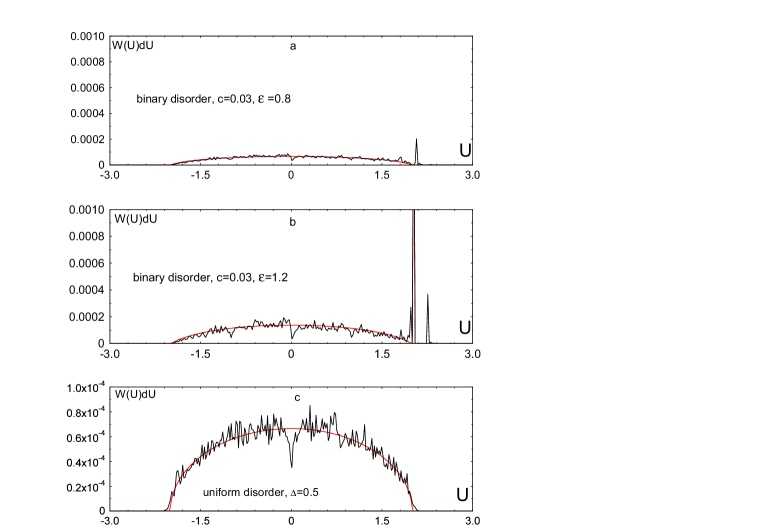
Figure 2: The ”participation” function – the comparison of theory (smooth curves) and computer simulation (noisy curves). For the case of binary disordered chain the occurrence of the peculiarity related to the edge state is seen: (a) – $\varepsilon=0.8<1$, no strong peculiarity, (b) – $\varepsilon=1.2>1$, sharp peak appear. (c) – the ”participation” function for the chain with uniform disorder at $\Delta=0.5$. $dU=1/50$ for all cases.

References

• (1) I. M. Lifshits, S. A. Gredeskul, and L. A. Pastur, Introduction to the Theory of Disordered Systems [in Russian], Nauka, Moscow (1982); English transl., Wiley, New York (1988).
• (2) Anderson P.W., Phys.Rev., v. 109, p. 1492, 1958.
• (3) A.V.Malyshev, V.A.Malyshev and F.Dominguez-Adame, arXiv:cond-mat/0303092.
• (4) Dyson F.J. Phys.Rev., v 92, p. 1331, 1953.
• (5) G.G.Kozlov, arXiv:0803.1920. [math-ph]