INTEGRAL/IBIS and Swift/XRT observations of hard cataclysmic variables

Abstract

The analysis of the third INTEGRAL/IBIS survey has revealed several new cataclysmic variables, most of which turned out to be intermediate polars, thus confirming that these objects are strong emitters in hard X-rays. Here we present high energy spectra of all 22 cataclysmic variables detected in the 3rd IBIS survey and provide the first average spectrum over the 20–100 keV band for this class. Our analysis indicates that the best-fit model is a thermal bremsstrahlung with an average temperature of $<kT>$ $\sim$22 keV. Recently, eleven (ten intermediate polars and one polar) of these systems have been followed-up by Swift/XRT (operating in the 0.3–10 keV energy band), thus allowing us to investigate their spectral behaviour over the range $\sim$0.3–100 keV. Thanks to this wide energy coverage, it was possible for these sources to simultaneously measure the soft and hard components and estimate their temperatures. The soft emission, thought to originate in the irradiated poles of the white dwarf atmosphere, is well described by a blackbody model with temperatures in the range $\sim$60–120 eV. The hard emission, which is supposed to be originated from optically thin plasma in the post-shock region above the magnetic poles, is indeed well modelled with a bremsstrahlung model with temperatures in the range $\sim$16–33 keV, similar to the values obtained from the INTEGRAL data alone. In several cases we also find the presence of a complex absorber: one totally (with $N_{\rm H}\sim(0.4-28)\times 10^{21}$ cm^-2) and one partially (with $N_{\rm H}\sim(0.7-9)\times 10^{23}$ cm^-2) covering the source. Only in four cases (V709 Cas, GK Per, IGR J06253+7334 and IGR J17303–0601), we find evidence for the presence of an iron line at 6.4 keV. We discuss our findings in the light of the systems parameters and cataclysmic variables/intermediate polars modelling scenario.

1 Introduction

Cataclysmic variables (CVs) are close binary systems, with orbital period typically less than one day, containing a white dwarf (WD) which is accreting material from a late-type main sequency secondary star filling its Roche lobe (for a review see Warner 1995). As the accreting matter falls onto the WD, it forms a disk; the infalling matter releases its gravitational energy, heating the accretion disk and the regions where matter falls onto the WD. As a result, radiation is emitted over many frequencies, from infrared to X-rays. Recently, this class of binaries has re-gained interest because of their detection in large numbers at energies above 20 keV, where very few cases were previously known thanks to RXTE (Suleimanov et al. 2005) and BeppoSAX (De Martino et al. 2004b) observations. CVs can be broadly divided into two subclasses: non magnetic and magnetic objects depending on the strength of the WD magnetic field.

In non-magnetic CVs (e.g. Dwarf Novae or DNe) the hard X-ray emission originates from the boundary layer between the accretion disk and the WD surface and depends on the mass accretion rate ($\dot{M}$) of the disk (Pringle & Savonije 1979). This boundary can release up to $50\%$ of the total accreting energy when the material decelerates on to the WD surface. For low $\dot{M}$ ($\lesssim 10^{16}$ g s^-1) the boundary is optically thin and emits hard X-rays with temperatures up to $10^{8}$ K. For high accretion rate ($\gtrsim 10^{16}$ g s^-1) the boundary layer is thick, thus suppressing hard X-rays and emitting mostly in soft X-rays with temperature $\sim$$10^{5}$ K (Pringle & Savonije 1979).

Magnetic cataclysmic variables (mCVs) are divided in two classes: polars (or AM Her type) and intermediate polars (IPs or DQ Her type). In polars (for a review see Cropper 1990) the magnetic field is so strong ($B>10^{7}$ Gauss, De Martino et al. 2004a) that it forces the WD to spin with the same period of the binary system ($P_{\rm rot,WD}=P_{\rm orb}$) and preventing the formation of an accretion disk around the WD. The infalling material is chanelled by the magnetic field along its lines and falls on the magnetic poles of the WD. In the IPs, instead, the weaker magnetic field ($B\sim 10^{6}-10^{7}$ Gauss, De Martino et al. 2004a) does not synchronize the spin period of the WD with the orbital period of the binary system ($P_{\rm rot,WD}<P_{\rm orb}$). In these objects, the accretion process is through a disk , which is truncated in its inner region because of the interaction with the WD magnetosphere; the overall result is the formation of an accretion curtain rather than a converging stream. In these systems, it is also likely that part of the material from the companion can flow directly on the magnetic poles without passing through the disk (disk-overflow, Hellier 1991).

In magnetic CVs the broad-band X-ray spectrum is mainly due to the superposition of a soft and a hard component. The hard X-ray emission is the consequence of the shock produced in the accreting material as it impacts the WD atmosphere. The hot post-shock region cools via thermal bremsstrahlung process emitting hard X-rays; the temperatures of the post-shock region are typically in the range $\sim$5–60 keV (Warner 1995; Hellier 2001). This emission is highly absorbed ($N_{\rm H}\sim 10^{23}$ cm^-2) within the accretion flow (Ishida et al. 1994) and is expected to be reflected by the WD surface (De Martino et al. 2004b and references therein). In polars, due to the strong magnetic field, cyclotron radiation cooling suppresses the high temperature bremsstrahlung emission of a substantial fraction of the electrons in the shock region (Lamb & Masters 1979; König, Beuermann & Gänsicke 2006). This may explain why most of hard X-ray detected CVs are IPs, in which cyclotron emission is negligible.

The soft X-ray component, originating by the reprocessing of the hard emission on the WD surface, is typically described by a blackbody emission with temperatures ranging from a few eV up to $\sim$100 eV (De Martino et al. 2004, 2006a,b). This component was mostly seen in polars but recently Evans & Hellier (2007), performing a systematic spectral analysis of XMM-Newton data of IPs, found this to be a common feature of IPs X-ray spectra. Furthermore, these authors suggest that the lack of a blackbody component in some of these systems is to be ascribed to geometrical effects: the accretion polar regions are either widely hidden by the accretion curtain or are only visible when foreshortened on the WD limb (depending on the inclination of the system).

Thanks to INTEGRAL observations strategy, a large number of new CVs have now been detected and classified through optical spectroscopy (Masetti et al. 2006,2008; Bikmaev et al. 2006; Gänsicke et al. 2005). In the third INTEGRAL/IBIS survey, 22 CVs are reported, confirming this class of binaries to be strong emitters in hard X-rays. In this paper we present IBIS spectral analysis of the entire sample of CVs detected by INTEGRAL. For eleven systems, which have been observed by Swift/XRT, we also report the broad-band ($\sim$0.3–100 keV) analysis by combining not simultaneous XRT and IBIS data. A detailed investigation of the temporal properties and of the spectral behaviour of the pulsations (i.e. the spectral analysis at the maximum and minimum of the pulse cycle) is beyond the aim of this paper. Therefore, here we only present the spectral analysis of the phase-averaged spectra.

2 Observation and data analysis

2.1 INTEGRAL

The INTEGRAL data reported here consist of several pointings performed by the IBIS/ISGRI instrument (Ubertini et al. 2003) between revolution 12 and 429, i.e. the period from launch to the end of April 2006. ISGRI images for each available pointing were generated in various energy bands using the ISDC offline scientific analysis software OSA v. 5.1 (Goldwurm et al. 2003). Count rates at the position of the source were extracted from individual images in order to provide light curves in various energy bands; from these light curves, average fluxes were then obtained and combined to produce an average source spectrum (see Bird et al. 2007 for details). Spectra were produced in nine energy bins over the 20–100 keV band. An appropriately re-binned rmf file was also produced from the standard IBIS spectral response file to match the pha file energy bins. Here and in the following, spectral analysis was performed with XSPEC v. 11.3.2 package (Arnaud 1996) and errors are quoted at 90% confidence level for one interesting parameter ($\Delta\chi^{2}=2.71$).

In Table 1 we list all 22 CVs detected so far by INTEGRAL together with their position and classification. As can be seen, this sample contains mainly magnetic systems (21 objects), with the majority ($\sim$81%, or 17 versus 4) being IPs (10 systems confirmed and seven possible/probable IP candidate, as reported in Table 1). Only one system (SS Cyg) is classified as DNe.

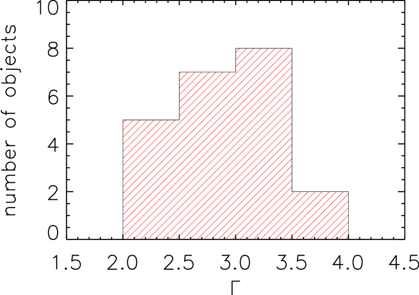
Figure 1: Photon index distribution of the whole IBIS CVs sample.

To characterise the hard X-ray emission (20–100 keV) of these systems, we fit the IBIS spectra with two models, a simple power law and a thermal bremsstrahlung. The results of these fits are reported in Table 1, where $\Gamma$, $kT$, 20–100 keV flux (assuming a bremsstrahlung model) and $\chi^{2}/\nu$ relative to both models are listed for each source. Generally, both models provide an acceptable fit, although in a few cases the bremmsstrahulung gives a better $\chi^{2}/\nu$. Inspection of Table 1 also indicates that there are no significant differences between the spectral parameters of the different classes of CVs. The photon index and temperatures distributions (shown in Figure 1 and Figure 2) peak at $\Gamma=2.9\pm 0.5$ and $kT=26.0\pm 11.0$ keV, respectively, in substantial agreement with what reported previously by Barlow et al. (2006) for a subsample. Thus, in order to improve the statistics, we fitted together all data sets allowing the flux to vary from source to source, but imposing the slope and the bremsstrahlung temperature to be the same for all objects. These fits yield a temperature of $kT=22.0\pm 0.9$ keV and a photon index $\Gamma=2.96\pm 0.05$, much in agreement with the mean values estimated from Figure 1 and Figure 2. Comparison of the $\chi^{2}/\nu$ strongly suggests that the thermal bremsstrahlung is the model that better reproduces the data ($\chi^{2}/\nu=272.6/175$) with respect the power law ($\chi^{2}/\nu=307/175$); this is reflected in the residuals to the models which are shown in Figure 3 and Figure 4. This result supports the hypothesis that the hard X-ray emission is due to a thermal bremsstrahlung component.

2.2 Swift/XRT

For eleven sources in our sample, we also have X-ray observations acquired with the XRT (X-ray Telescope, 0.2–10 keV, Burrows et al. 2005) on board the Swift satellite (Gehrels et al. 2004). XRT data reduction was performed using the XRTDAS standard data pipeline package (xrtpipeline v. 0.10.6), except for the observations performed after August 2007 (in these cases we used the latest version 0.11.6 of the pipeline), in order to produce screened event files. All data were extracted only in the Photon Counting (PC) mode (Hill et al. 2004), adopting the standard grade filtering (0–12 for PC) according to the XRT nomenclature. The log of all X-ray observations, available at June 2 2008, is given in Table 2. For each measurement, we report the XRT observation date, the total on-source exposure time and the total net count rate in the 0.3–10 keV energy band.

For those sources in which the XRT count rate was high enough to produce event pile-up, we extracted the events in an annulus centered on the source, by determining the size of the inner circle according to the procedure described in Romano et al. (2006). In the other cases, events for spectral analysis were extracted within a circular region of radius 20^′′, centered on the source position, which encloses about 90% of the PSF at 1.5 keV (see Moretti et al. 2004).

The background was taken from various source-free regions close to the X-ray source of interest, using circular regions with different radii in order to ensure an evenly sampled background. In all cases, the spectra were extracted from the corresponding event files using the XSELECT software and binned using grppha in an appropriate way, so that the $\chi^{2}$ statistic could be applied. We used version v.009 of the response matrices and create individual ancillary response files arf using xrtmkarf v. 0.5.6.

We summed together all the available observations for each source to provide an average source spectrum as done for the INTEGRAL/IBIS data. A posteriori, this approach proved resonable since only in two cases (V709 Cas and GK Per) we observed significant changes in flux, by a factor of 1.5 and 1.7 respectively, but not in shape.

3 The broad-band spectral analysis

Use of broad-band data is particularly important to determine the properties of the emitting regions, in particular the temperature of the optically thin plasma, the presence of interstellar and/or circumstellar absorption; it is also useful to study the effects of reprocessing of the hard X-ray emission on the WD surface. The basic model we adopted consists of a blackbody ($kT_{\rm BB}$) and a bremsstrahlung ($kT_{\rm Brems}$) component to account for the soft and hard X-ray emissions expected in magnetic CVs, plus two cold media consisting of a simple absorber, totally covering the source (with a column density $N_{\rm H}$) and a partial covering absorber (with a column density $N_{\rm H(pc)}$ and covering factor $C_{\rm F}$). If required by the data, we also included in the model another emission component consisting of an optically thin plasma (MEKAL code in XSPEC) and a K$\alpha$ iron line. We also tested the data for the presence of a multi-temperature structure of the post-shock region and of a reflection component, but the data were of too low statistical quality to allow these more complex fits. We introduced in the fitting procedure a cross-calibration constant ($C_{\rm calib}$) to account for possible mismatch between XRT and IBIS data as well as for source flux variations. The results of the spectral fits including cross-calibration constant and reduced $\chi^{2}$ are all listed in Table 3; spectra and residuals with respect to the best-fit model are plotted in Figure 5. We found that in most cases our basic model provides a good description of the broad-band spectra of our CVs. The cross-calibration constants have been found to be consistent, within the uncertainties, with unity for all sources apart from GK Per, in which the low value of the constant can be ascribed to the flux variability of the source, as confirmed by XRT (this work) and previous observations (Vrielmann, Ness & Schmitt 2005 and references therein). Three systems out of eleven (XSS J12270-4859, IGR J16500–3307 and IGR J17195–4100) do not show evidence for complex absorption, but this could be due to the short exposure of the XRT observations. In eight cases (V709 Cas, IGR J06253+7334, XSS J12270–4859, IGR J14536–5522, IGR J15479–4529, IGR J16167–4957, IGR J17195–4100 and IGR J17303–0601) the column density of the fully covering absorber is lower or compatible with the Galactic absorption in the direction of the sources, suggesting an interstellar origin for this component. For systems showing the partial covering absorption, we found that the absorber is remarkably higher than the galactic one, indicating an intrinsic origin likely associated to the presence of the accretion material along the line of sight. The range of values found for both total and partial absorber are consistent with what found by Evans $\&$ Hellier (2007) by analysing the XMM-Newton data of several IPs. Only in four cases (V709 Cas, GK Per, IGR J06253+7334 and IGR J17303-0601) we find evidence for the presence of an iron line at around 6.4 keV; lack of iron line detection in the other sources may be due to the lower statistical quality of their X-ray data.

An interesting result of our analysis is that most of the IPs of our sample significantly require a blackbody component (see Table 4); the temperatures related to this component are all in the range 60–120 eV as observed in previous studies (Evans & Hellier (2007); De Martino et al. 2001,2004b,2006b,2008). Following Evans $\&$ Hellier (2007), we would not expect to observe a blackbody component if the partial covering absorption is associated to the accretion curtain; however, in our case the blackbody emission does not seem to be affected by the strength of the partial absorber and is observed in all CVs. The fact that in FO Aqr we can determine the blackbody temparature, while Evans & Hellier (2007) do not, may be related to our broad-band analysis which allows a better definition of the source continuum and an estimate of the soft component temperature. A bremmsstrahulung component is required in every object and its temperature ranging from 16–35 keV, is generally consistent with values obtained using IBIS data alone.

4 Notes on a few individual sources

V709 Cas: in this case our results are in agreement with what found by Falanga et al. (2005) from a joint JEM-X/ISGRI spectrum. We confirm a temperature for the hard X-ray emission at around 25 keV, without claiming the presence of a reflection component as instead reported by De Martino et al. (2001), even if we fit the data assuming their model. In this case the data shows an excess at around 6.4 keV, that we modeled by adding an iron line to the basic model (see Table 3). The addition of this component is required by the data at 99.99$\%$ confidence level and provides an energy centroid $E=6.46^{+0.05}_{-0.04}$ keV and an $EW=140^{+46}_{-55}$ eV, which is consistent with the value reported by De Martino et al. (2001).
GK per: a recent analysis of XMM-Newton data of GK Per has revealed the presence of spectral complexity in the soft energy band, which has been resolved in a multitude of emission lines thanks to the high-resolution spectroscopy performed with the RGS (Vrielmann et al. 2005). Furthermore, the image of the source taken with the ACIS-S detector on board Chandra, reported by the same authors, shows the presence of extended emission (a shell with a radius of $\sim$$50$ arcsec) around the source, which disappears above $\sim$1.5 keV. With the XRT data we cannot evaluate the contribution of this component to the total emission, therefore we decided to perform the spectral analysis above $\sim$1 keV. The fit with the basic model is not satisfactory ($\chi^{2}/\nu=693.2/502$): the residuals to the model show a clear excess of counts around $\sim$6 keV. The iron K$\alpha$ region of this source has been recently resolved by Chandra in three distinct components (6.4, 6.7 and 6.97 keV, Hellier & Mukai (2004)), with the fluorescent line showing a red wing up to 6.33 keV. This last component has been confirmed by XMM-Newton observations (Vrielmann et al. 2005). In our analysis, the addition of a Gaussian Fe K$\alpha$ line is strongly required by the data ($>99.99\%$, $\Delta\chi^{2}=183$ for three degrees of freedom) and gives an energy centroid $E=6.35^{+0.05}_{-0.03}$ keV, a line width $\sigma=0.29^{+0.05}_{-0.04}$ keV and an equivalent width $EW=371^{+59}_{-53}$ eV, in agreement with what reported by Vrielmann et al. (2005). The confidence contours of the line energy versus line width are shown in Figure 6. Unfortunately, because of the low sensitivity of XRT in this energy band, we cannot further resolve this spectral region to verify the presence of other lines and/or of a red wing in the neutral iron line.
IGR J06253+7334: in this case, although the basic model provides a good description of the data ($\chi^{2}/\nu=111.8/121$), an excess at around 6.4 keV is clearly evident. The addition of a narrow Gaussian line at 6.4 keV is required by the data at 99.5% confidence level ($\Delta\chi^{2}=7.3$ for one degree of freedom) and provides an $EW=195^{-108}_{+115}$ eV (see Table 3). By leaving the iron line energy free to vary, we found an energy centroid $E=6.41^{+0.06}_{-0.04}$, a similar $EW$, but a lower significance of the line (98.4% confidence level). Concerning the temperature of the bremsstrahlung component, we found a difference between the value found by fitting the IBIS data alone ($\sim$7 keV) and that found in the broad-band spectral analysis ($\sim$35 keV). This discrepancy could be due to a source variation between XRT and IBIS observations, or perhaps it was the use of a more complex model which resulted in the different parameter value.
IGR J17303–0601: also for this source the basic model does not reproduce satisfactorily the spectrum ($\chi^{2}/\nu=358/292$). The addition of a further emission component consisting of an optically thin plasma (MEKAL code in XSPEC) improves the fit ($\Delta\chi^{2}=38$ for two degrees of freedom) and is significant at 99.99%, giving a temperature $kT=0.20^{+0.03}_{-0.02}$ keV. The addition of a narrow Gaussian line at 6.4 keV to account for the excess at around 6 keV is only marginally required by the data ($\sim$$95\%$) and provides an $EW=83^{+60}_{-65}$ eV. Our results are consistent with those recently reported by De Martino et al. (2008) from a combined analysis of XMM-Newton and INTEGRAL data, except for the temperature of the hard X-ray emission (which is lower in our fit than in theirs) and the metal abundances, which we freeze to the solar value because of the lack of statistics.

5 Discussion

We have analysed INTEGRAL data of a sample of 22 hard X-ray selected CVs, the majority of which are IPs. We confirm previous indications that the high energy spectra of these type of objects are well described by either a bremsstrahlung model with $kT$ in the range 7–56 keV or a power law with $\Gamma$ in the range 2.1–3.5; however, the average INTEGRAL spectrum of all 22 CVs is significantly better fitted by the bremsstrahlung model with an average temperature of 22 keV. Confirmation that IPs are the most powerful soft gamma-ray emitters within the CV population is an important result defined from INTEGRAL observations. The lack of emission above a few tens of keV from a large set of non-magnetic white dwarf binaries and synchronised polars is also an interesting information. For non-magnetic CVs the non detection of high energy emission could be related to the lack of radial accretion flow. Instead, the fact that IPs are high energy emitters and polars are not suggests that the onset of emission above 10 keV requires some level of synchronisation of the orbital and spin periods, but then the high energy radiation is less likely to be observed when full synchronisation sets in. One would then expect to observe some level of correlation between the characteristics of the soft gamma-ray emission and the degree of synchronisation. In Table 5 we report for each source in the complete sample of CVs those parameters which characterise the system; data are obtained from the literature (see references in Table 5) and include the orbital and spin periods and their ratio, the WD mass and the source distance. Not all sources are fully characterised and in the cases of newly discovered INTEGRAL sources data are often unavailable. As a first step we cross-correlated the bremsstrahlung temperature and 20–100 keV flux as obtained in Table 1 with the various parameters listed in Table 5, but have not found any convincing correlations. In particular, neither of these two gamma-ray parameters cross correlate with the ratio of spin to orbital period: while a wide range (extending from around 0.02 to up $\sim$1) in the degree of synchronisation is apparent in the sample studied, yet there is a notable similarity in the thermal bremsstrahlung temperatures throughout the sample. It remains to understand how systems which are quite different in various parameters are able to privide such a well confined range of bremsstrahlung temperatures.

Half of the sources in the sample have also X-ray data available so that the low energy emission could be parametrized in terms of a blackbody model with well constrained temperatures in the range 60–120 eV. Extra features to this baseline model have been found in a few sources such as an iron line at 6.4 keV in four sources and an extra thermal component in one object. Both soft and hard components are viewed through two layers of neutral absorbing material: the first seen in all 11 objects totally covers the emitting region, while the second, seen in $\sim$70% of them, only partially covers the source. We also searched for correlation between the system values and soft X-ray emission parameters but again found none. The measured X-ray (2–10 keV) and soft gamma-ray (20–100 keV) luminosities are found to span from 10³² to 10³³ erg s^-1; their ratios span from 0.02 to 7.5 with an average at around 1.3, but only when GK Per, with a ratio of $\sim$38, is discounted. GK Per stands out in the sample because it has a considerably longer orbital period than the rest of the group and, by a considerable margin, the highest X-ray to gamma-ray flux ratio. GK Per was a bright nova occurring in 1901 in Perseus and is now classified as an IP. It is possible that the system is still quite young and has not fully switched into the standard IP state as described here; coverage in time would be extremely interesting to see if any change towards a more standard IP behaviour will take place. The bolometric luminosities of the blackbody emitting components have corresponding emitting areas in the range $10^{12}$ to $\sim$$10^{16}$ cm², with GK Per and FO Aqr located at the top end of the range. From the available values of the WD mass, we estimate that the observed blackbody emitting area covers from $\sim$$3\times 10^{-3}$ to $\sim$$9\times 10^{-7}$ of the WD surface.

Finally, it is important to underline that a unique baseline model has been able to describe the broad-band (0.3–100 keV) data of half the sample of INTEGRAL detected objects. This model is consistent with the standard IP scenario, where thermal emission originating in the irradiated poles of the WD atmosphere provides the soft X-ray component, while emission in the post-shock region above the magnetic poles gives rise to the thermal bremsstrahlung component; this emission is absorbed within the accretion flow and is possibly reflected by the WD surface, hence the production of iron line features. This baseline model can be used as a pointer to IP classification (Ramsay et al. 2008) and considered a signature of such systems within the CVs population.

Table 1: Characteristics of the CVs belonging to the third IBIS Survey and their best-fit IBIS parameters by assuming power law and bremsstrahlung models.

Source	RA	Dec	Classa,b	$\Gamma$	$\chi^{2}/\nu$	kTBrems	$\chi^{2}/\nu$	F(20–100 keV)c
	(J2000)	(J2000)				(keV)		($10^{-11}$ erg cm-2 s-1)
IGR J00234+6141	5.726	+61.706	IP∙	$2.18^{+1.24}_{-1.04}$	14.0/7	$>$14	13.8/7	0.6
V709 Cas	7.204	+59.306	IP∙	$2.77^{+0.13}_{-0.12}$	13.2/7	$25.5^{+3.1}_{-2.7}$	3.9/7	5.0
GK Per	52.778	+43.934	IP∙	$2.21^{+0.84}_{-0.72}$	4.6/7	$43.7^{+128.8}_{-23.4}$	3.6/7	2.1
BY Cam	85.737	+60.850	P	$2.40^{+1.08}_{-0.87}$	5.4/7	$36.7^{+230.3}_{-22.7}$	5.9/7	3.2
IGR J06253+7334	96.340	+73.602	IP∙	$>3.5$	2.2/7	$7.0^{+8.9}_{-3.8}$	2.2/7	0.7
XSS J12270–4859	187.007	–48.893	IP∙∙∙	$2.29^{+0.49}_{-0.44}$	9.1/7	$42.5^{+36.0}_{-15.8}$	6.6/7	2.5
V834 Cen	212.249	–45.273	P	$3.00^{+1.77}_{-1.28}$	6.8/7	$18.7^{+61.0}_{-10.6}$	6.8/7	0.7
IGR J14536–5522	223.435	–55.374	P	$3.58^{+0.61}_{-0.52}$	7.1/7	$14.0^{+5.4}_{-3.7}$	8.1/7	1.4
IGR J15094–6649	227.351	–66.844	IP∙∙∙	$3.16^{+0.67}_{-0.55}$	3.8/7	$18.8^{+11.5}_{-6.5}$	6.5/7	1.7
IGR J15479–4529	237.050	–45.478	IP∙	$2.64^{+0.13}_{-0.12}$	29.3/7	$29.3^{+3.1}_{-2.7}$	6.2/7	6.1
IGR J16167–4957	244.140	–49.974	IP∙∙∙	$3.28^{+0.27}_{-0.25}$	10.5/7	$17.3^{+3.3}_{-2.7}$	10.0/7	2.3
IGR J16500–3307	252.491	–33.064	IP∙∙,d	$3.18^{+0.47}_{-0.40}$	18.8/7	$20.0^{+6.9}_{-4.7}$	14.5/7	1.5
V2400 Oph	258.172	–24.280	IP∙	$3.29^{+0.15}_{-0.14}$	13.7/7	$16.6^{+1.9}_{-1.7}$	8.7/7	3.3
IGR J17195–4100	259.906	–41.014	IP∙∙	$2.86^{+0.19}_{-0.18}$	8.8/7	$25.0^{+4.6}_{-3.6}$	19.4/7	3.5
IGR J17303–0601	262.596	–5.988	IP∙	$2.56^{+0.32}_{-0.29}$	7.5/7	$32.4^{+12.5}_{-8.1}$	8.8/7	4.5
V2487 Oph	262.963	–19.233	IP∙∙∙	$2.12^{+0.51}_{-0.47}$	4.4/7	$55.6^{+76.4}_{-24.5}$	3.6/7	1.2
V1223 Sgr	283.755	–31.154	IP∙	$3.26^{+0.13}_{-0.12}$	10.5/7	$17.7^{+1.6}_{-1.4}$	3.1/7	7.1
V1432 Aql	295.058	–10.428	P	$2.82^{+0.56}_{-0.49}$	4.8/7	$24.4^{+15.3}_{-8.1}$	5.1/7	3.4
V2069 Cyg	320.906	+42.278	IP∙∙	$3.20^{+0.76}_{-0.60}$	4.6/7	$19.2^{+12.3}_{-6.8}$	4.5/7	1.2
IGR J21335+5105	323.438	+51.121	IP∙	$2.91^{+0.25}_{-0.24}$	22.0/7	$23.6^{+5.0}_{-4.0}$	12.4/7	4.1
SS Cyg	325.691	+43.583	DN	$3.19^{+0.27}_{-0.25}$	2.7/7	$18.4^{+3.7}_{-2.9}$	4.8/7	3.7
FO Aqr	334.478	–8.317	IP∙	$2.70^{+1.28}_{-0.89}$	7.5/7	$29.7^{+70.1}_{-16.6}$	7.8/7	4.2

• ^a IP: intermediate polar; P: polar; DN: dwarf nova;
  ^b The classification of the IP systems is addressed following the Koji Mukai’s IP probability classification (available at http://asd.gsfc.nasa.gov/Koji.Mukai/iphome/catalog/alpha.html): ^∙: confirmed; ^∙∙: probable; ^∙∙∙: possible;
  ^c The flux is derived by assuming the bremsstrahlung model;
  ^d For this source we used the classification proposed by Masetti et al. (2008).

Table 2: Log of the Swift XRT observations used in this paper (until June 2, 2008).

Source	Obs date	Exposurea	Count rate (0.3–10 keV)
		(s)	(counts s-1)
V709 Cas	Jul 15, 2007	290	$0.245\pm 0.029$
	Jul 17, 2007	1156	$0.415\pm 0.019$
	Nov 04, 2007	3970	$0.497\pm 0.011$
	Nov 04, 2007	3532	$0.396\pm 0.011$
	Nov 05, 2007	2370	$0.453\pm 0.014$
	Nov 14, 2007	2985	$0.451\pm 0.012$
	Apr 07, 2008	5732	$0.437\pm 0.009$
	Apr 08, 2008	1376	$0.437\pm 0.020$
	May 01, 2008	1651	$0.430\pm 0.016$
	Jun 01, 2008	6365	$0.492\pm 0.009$
total obs	–	29427	$0.456\pm 0.004$
GK Per	Dec 20, 2006	3931	$0.883\pm 0.015$
	Dec 26, 2006	4493	$0.445\pm 0.010$
	Jan 02, 2007	4679	$0.482\pm 0.010$
	Jan 09, 2007	4802	$0.455\pm 0.010$
	Jan 19, 2007	5993	$0.460\pm 0.009$
	Jan 23, 2007	5756	$0.480\pm 0.009$
	Jan 30, 2007	966	$0.403\pm 0.020$
	Feb 04, 2007	3921	$0.429\pm 0.010$
	Feb 08, 2007	5229	$0.464\pm 0.009$
	Feb 12, 2007	2956	$0.410\pm 0.012$
	Feb 16, 2007	6131	$0.424\pm 0.008$
	Feb 19, 2007	2787	$0.465\pm 0.013$
	Feb 23, 2007	3226	$0.484\pm 0.012$
	Feb 26, 2007	6346	$0.481\pm 0.009$
	Mar 02, 2007	3132	$0.428\pm 0.012$
	Mar 06, 2007	7765	$0.448\pm 0.008$
	Mar 09, 2007	4185	$0.469\pm 0.011$
	Mar 13, 2007	5869	$0.443\pm 0.009$
	Sep 27, 2007	2470	$0.294\pm 0.011$
total obs	–	84637	$0.475\pm 0.002$
IGR J06253+7334	Nov 04, 2007	3411	$0.114\pm 0.006$
	Dec 03, 2007	4468	$0.114\pm 0.005$
	Dec 05, 2007	10092	$0.123\pm 0.003$
	Dec 06, 2007	8928	$0.084\pm 0.003$
total obs	–	26899	$0.114\pm 0.006$
XSS J12270–4859	Sep 15, 2005	4965	$0.269\pm 0.007$
	Sep 24, 2005	1870	$0.191\pm 0.010$
total obs	–	6835	$0.251\pm 0.006$
IGR J14536–5522	Oct 10, 2005	7165	$0.395\pm 0.008$
	Mar 06, 2006	2040	$0.321\pm 0.013$
total obs	–	9205	$0.383\pm 0.007$
IGR J15479–4529	Jun 22, 2007	359	$0.405\pm 0.034$
	Jun 24, 2007	3978	$0.369\pm 0.010$
	Jun 26, 2007	1002	$0.289\pm 0.017$
	Jan 25, 2008	4772	$0.485\pm 0.010$
total obs	–	10111	$0.430\pm 0.007$
IGR J16167–4957	Sep 09, 2005	2434	$0.167\pm 0.008$
	Jan 26, 2006	3087	$0.182\pm 0.008$
	Feb 15, 2007	5189	$0.185\pm 0.006$
total obs	–	10710	$0.184\pm 0.004$
IGR J16500–3307	Jan 27, 2007	4594	$0.136\pm 0.005$

Source	Obs date	Exposurea	Count rate (0.3–10 keV)
		(s)	(counts s-1)
IGR J17195–4100	Oct 29, 2005	3474	$0.434\pm 0.011$
	Oct 30, 2005	1588	$0.455\pm 0.017$
	Jun 21, 2007	719	$0.400\pm 0.024$
	Apr 30, 2008	7323	$0.462\pm 0.001$
	May 02, 2008	2727	$0.459\pm 0.012$
total obs	–	15831	$0.456\pm 0.005$
IGR J17303–0601	Feb 22, 2007	6520	$0.369\pm 0.008$
	Feb 23, 2007	11040	$0.398\pm 0.006$
	Feb 25, 2007	4213	$0.461\pm 0.010$
	Feb 28, 2007	817	$0.548\pm 0.026$
	Mar 02, 2007	2043	$0.456\pm 0.015$
total obs	–	24633	$0.411\pm 0.004$
FO Aqr	May 04, 2006	9939	$0.316\pm 0.006$
	May 04, 2006	3894	$0.328\pm 0.009$
	May 04, 2006	1189	$0.256\pm 0.015$
	May 04, 2006	5454	$0.244\pm 0.007$
total obs	–	20476	$0.292\pm 0.004$

• ^a Total on-source exposure time.

Table 3: XRT/IBIS spectral analysis results of sources fitted with the basic model (see text). Frozen parameters are written between squared brackets.

Source	Energy band	$N_{\rm H}$	$N_{\rm H(pc)}$	$C_{\rm F}$	kTBB	kTBrems	F${}_{\rm 2-10~{}keV}$	F${}_{\rm 20-100~{}keV}$	$C_{\rm calib}$a	$\chi^{2}/\nu$
	(keV)	($10^{22}$ cm-2)	($10^{22}$ cm-2)		(eV)	(keV)	($10^{-11}$ erg cm-2 s-1)	($10^{-11}$ erg cm-2 s-1)
V709 Casb	0.3–100	0.23${}^{+0.10}_{-0.04}$	12.0${}^{+11.0}_{-5.6}$	0.28${}^{+0.07}_{-0.06}$	84${}^{+6}_{-8}$	25.6${}^{+2.7}_{-2.4}$	3.1	5.0	$1.54^{+0.22}_{-0.22}$	325.8/329
GK Perc	1–100	2.8${}^{+0.24}_{-0.12}$	16.8${}^{+2.4}_{-1.7}$	0.69${}^{+0.03}_{-0.02}$	82${}^{+6}_{-8}$	23.0${}^{+9.2}_{-6.5}$	16.0	2.0	$0.12^{+0.07}_{-0.04}$	510.5/499
IGR J06253+7334d	0.3–100	0.06${}^{+0.10}_{-0.01}$	6.7${}^{+4.7}_{-3.0}$	0.62${}^{+0.08}_{-0.10}$	65${}^{+8}_{-5}$	$29.4^{+16.0}_{-9.0}$	0.7	1.1	$1.16^{+0.92}_{-0.57}$	104.5/120
XSS J12270–4859	0.4–100	0.037${}^{+0.025}_{-0.023}$	–	–	$<$ 127	33.4${}^{+18.4}_{-10.6}$	1.2	2.3	$1.60^{+0.88}_{-0.56}$	75.3/76
IGR J14536–5522	0.3–100	0.071${}^{+0.07}_{-0.03}$	12.2${}^{+8.3}_{-6.0}$	0.58${}^{+0.08}_{-0.09}$	60${}^{+7}_{-5}$	16.3${}^{+5.0}_{-4.0}$	2.4	1.5	$1.03^{+0.65}_{-0.40}$	130.4/140
IGR J15479–4529	0.3–100	0.065${}^{+0.014}_{-0.008}$	14.6${}^{+8.3}_{-3.7}$	0.52${}^{+0.08}_{-0.07}$	101${}^{+12}_{-10}$	28.4${}^{+3.2}_{-2.8}$	2.4	6.1	$1.82^{+0.36}_{-0.34}$	116.4/108
IGR J16167–4957	0.6–100	0.96${}^{+0.15}_{-0.12}$	94.0${}^{+42.7}_{-37.2}$	0.84${}^{+0.11}_{-0.34}$	95${}^{+15}_{-12}$	16.7${}^{+6.6}_{-4.5}$	1.7	2.3	$0.75^{+1.74}_{-0.36}$	94.0/86
IGR J16500–3307	0.9–50	1.88${}^{+0.73}_{-0.64}$	–	–	119${}^{+28}_{-22}$	32.0${}^{+31}_{-11}$	1.1	1.9	$1.25^{+0.81}_{-0.52}$	46.7/30
IGR J17195–4100	0.3–100	0.23${}^{+0.04}_{-0.06}$	–	–	104${}^{+12}_{-11}$	29.7${}^{+5.4}_{-4.2}$	2.4	3.6	$1.35^{+0.31}_{-0.26}$	263.3/263
IGR J17303–0601e	0.3–100	0.20${}^{+0.04}_{-0.02}$	45.2${}^{+25.1}_{-18.6}$	0.52${}^{+0.14}_{-0.12}$	85${}^{+9}_{-12}$	31.6${}^{+12.7}_{-7.8}$	1.9	4.4	$1.22^{+0.59}_{-0.49}$	320.0/290
FO Aqr	0.4–50	0.78${}^{+0.19}_{-0.18}$	7.2${}^{+1.2}_{-0.9}$	0.82${}^{+0.04}_{-0.03}$	61${}^{+8}_{-6}$	[29.7]f	3.6	2.1	$0.75^{+0.22}_{-0.21}$	155.7/169

^a XRT/IBIS cross-calibration constant;
^b For this source the fit also includes a narrow Gaussian line at $E=6.46^{+0.05}_{-0.04}$ keV with $EW=141^{+43}_{-58}$ eV (see text for details);
^c For this source the fit also includes a Gaussian iron line at $E=6.35^{+0.05}_{-0.03}$ keV with $\sigma=0.29^{+0.05}_{-0.04}$ keV and $EW=371^{+59}_{-53}$ eV (see text for details);
^d For this source the fit also includes a narrow Gaussian line at 6.4 keV with $EW=195^{+115}_{-108}$ eV (see text for details);
^e For this source the fit also includes a further thermal component (MEKAL code) with $kT=0.21^{+0.01}_{-0.02}$ keV (see text for details);
^f Fixed at the value obtained by fitting the IBIS spectrum alone.

Table 4: Fit statistics for each source with and without the blackbody component.

Source	$\chi^{2}/\nu$		$F$–test
	No BB	with BB
V709 Cas	349.2/331	325.8/329	$1.12\times 10^{-5}$
GK Per	615.2/501	510.5/499	$6.10\times 10^{-21}$
IGR J06253+7334	173.4/122	104.5/120	$6.37\times 10^{-14}$
XSS J12270–4859	81.2/78	75.3/76	$5.69\times 10^{-2}$
IGR J14536–5522	434.4/142	130.4/140	$2.66\times 10^{-37}$
IGR J15479–4529	182.1/108	116.1/106	$4.36\times 10^{-11}$
IGR J16167–4957	103.0/88	94.0/86	$1.96\times 10^{-2}$
IGR J16500–3307	64.2/32	46.7/30	$8.45\times 10^{-3}$
IGR J17195–4100	277.0/265	263.3/263	$1.27\times 10^{-3}$
IGR J17303–0601	417.4/292	320.0/290	$1.85\times 10^{-17}$
FO Aqr	190.3/171	155.7/169	$4.32\times 10^{-8}$

Table 5: Table of characteristics of the CVs observed by INTEGRAL.

Source	Porb	Pspin	Pspin/Porb	Mass	Dist	Refs
	(min)	(s)		(M☉)	(pc)
IGR J00234+6141	$242.0\pm 0.3$	$563.53\pm 0.62$	0.04	–	530	1
V709 Cas	320.4	312.7	0.0167	$0.90\pm 0.10$	$230\pm 20$	2, 3
GK Per	2875.2	351.34	0.00204	$0.92^{+0.39}_{-0.13}$	420	2, 4
BY Cam	201.3	11846.4	0.981	$\geq 0.8$	190	2, 5
IGR J06253+7334	283	1186.7	0.07	0.8	500	2, 6, 7
XSS J12270–4859	–	–	–	–	220	8
V834 Cen	101.4	–	–	$0.70^{+0.20}_{-0.15}$	80	2, 9
IGR J14536–5522	–	–	–	–	190	8
IGR J15094-6649	–	–	–	–	140	8
IGR J15479–4529	562	693	0.021	$\geq 0.5$	540–840	2, 9
IGR J16167–4957	–	–	–	–	170	8
IGR J16500–3307	–	–	–	–	$\sim$210	10
V2400 Oph	205.2	927	0.075	$0.69^{+0.06}_{-0.24}$	300	2, 4
IGR J17195–4100	–	–	–	–	110	8
IGR J17303–0601	924	128	0.0023	0.89–1.02	–	11
V2487 Oph	–	–	–	–	–	12
V1223 Sgr	201.9	745.6	0.062	$1.046^{+0.049}_{-0.012}$	527	2, 13
V1432 Aql	201.94	12150.4	1.003	$1.2\pm 0.2$	230	2, 14
V2069 Cyg	448.8	–	–	–	1650	2
IGR J21335+5105	431.6	570.8	0.022	0.6–1.0	1400	2, 15
SS Cyg	396.2	–	–	–	166	2
FO Aqr	291	1254.5	0.0718	$1.19^{+0.11}_{-0.31}$	400	3, 16

• References: [1] Bonnet-Bidaud et al. (2007); [2] Barlow et al. (2006) and references therein; [3] Suleimanov et al. (2005); [4] Evans & Hellier (2007); [5] Schwarz et al. (2005); [6] Staude et al. (2003); [7] Araujo-Betancor et al. (2003); [8] Masetti et al. (2006); [9] De Martino et al. (2006b); [10] Masetti et al. (2008); [11] De Martino et al. (2008); [12] Hernanz & Sala (2002); [13] Beuermann et al. (2004); [14] Rana et al. (2005); [15] Bonnet-Bidaud et al. (2006); [16] Norton et al. (2004).

Figure 2: Temperature distribution of the whole IBIS CVs sample.

Figure 3: IBIS average spectrum fitted with a simple power law (upper panel); residuals to this model are in units of $\sigma$ (lower panel).

Figure 4: IBIS average spectrum fitted with a bremsstrahlung model (upper panel); residuals to this model are in units of $\sigma$ (lower panel).

Figure 5: Best-fit model of the XRT/IBIS phase-averaged spectrum of the eleven systems followed-up by Swift, as described in Table 3 (upper panel); residuals to this model are in units of $\sigma$ (lower panel).

Figure 5: -Continued

Figure 6: Confidence contours (at 68%, 90%, and 99% confidence level) of the iron line energy versus line width for the best-fit model of GK Per.

References

- Araujo-Betancor et al. (2003) Araujo-Betancor, S., Gänsicke, B. T, Hagen, H.–J, Rodriguez-Gil, P., & Engels, D. 2003, A&A, 406, 213
- Arnaud (1996) Arnaud K. A. 1996, XSPEC: the first ten years, in Astronomical Data Analysis Software and Systems V, ed. G. H. Jacoby, & J. Barnes, ASP Conf Ser. 101, 17
- Barlow et al. (2006) Barlow, E. J., Knigge, C., Bird A. J., et al. 2006, MNRAS, 372, 224
- Beuermann et al. (2004) Beuermann, K., Harrison, Th. E., McArthur, B. E., Benedict, G. F., & Gänsicke, B. T. 2004, A&A, 419, 291
- Bird et al. (2007) Bird, A. J., Malizia, A., Bazzano, A., et al. 2007, ApJS, 170, 175
- Bikmaev et al. (2006) Bikmaev, I. F., Revnivtsev, M. G., Burenin, R. A. & Sunyaev, R. A. 2006, Astr. Letters, 32, 588
- Bonnet-Bidaud et al. (2007) Bonnet-Bidaud, J.–M., De Martino, D., Falanga, M., Mouchet, M., & Masetti N. 2007, A&A, 473, 185
- Bonnet-Bidaud et al. (2006) Bonnet-Bidaud, J.–M., Mouchet, M., De Martino, D., Silvotti, R., & Motch, C 2006, A&A, 445, 103
- Burrows et al. (2005) Burrows, D. N., Hill, J. E., Nousek, J. A., et al. 2005, Space Sci. Rev., 120, 165
- Cropper (1990) Cropper, M. 1990, Space Sci. Rev., 54, 195
- De Martino et al. (2008) De Martino, D., Matt, G. Mukai, K., et al. 2008, A&A, 481, 149
- De Martino et al. (2006a) De Martino, D., Matt, G., Mukai, K., Bonnet-Bidaud, J.–M., Burwitz, V., Gänsicke, B. T., Haberl, F., & Mouchet, M. 2006a, A&A, 454, 287
- De Martino et al. (2006b) De Martino, D., Bonnet-Bidaud, J.–M., Mouchet, M., Gänsicke, B. T., Haberl, F., & Motch, C. 2006b, A&A, 449, 115
- De Martino et al. (2004a) De Martino, D., Matt, G., Belloni, T., Chiappetti, L., Haberl, F., & Mukai, K. 2004a, Nuc. Phys. B Proc. Supp., 132, 693
- De Martino et al. (2004b) De Martino, D., Matt, G., Belloni, T., Haberl, F. & Mukai, K. 2004b, A&A, 415, 1009
- De Martino et al. (2001) De Martino, D., Matt, G. Mukai, K., et al. 2001, A&A, 377, 499
- Evans & Hellier (2007) Evans, P. E. & Hellier, C. 2007, ApJ, 663, 1277
- Falanga et al. (2005) Falanga, M., Bonnet-Bidaud, J. M. & Suleimanov, V. 2005, A&A, 444, 561
- Gehrels et al. (2004) Gehrels, N., Chincarini, G., Giommi, P. et al. 2004, ApJ, 611, 1005
- Gänsicke et al. (2005) Gänsicke, B. T., Marsh, T. R., Edge, A., et al. 2005, Atel 463
- Goldwurm et al. (2003) Goldwurm, A., David, P., Foschini, L., et al. 2003, A&A, 411, L223
- Hellier et al. (2004) Hellier, C., & Mukai, K. 2004, MNRAS, 352, 1037
- Hellier (1991) Hellier, C. 2001, Cataclysmic Variables Stars (Springer-Praxis: Chichester)
- Hellier (1991) Hellier, C. 1991, MNRAS, 251, 693
- Hernanz & Sala (2002) Hernanz, M., & Sala, G. 2002, Science, 298, 393
- Hill et al. (2004) Hill, J. E., Burrows, D. N., Nousek, J. A., et al. 2004, Proc. SPIE, 5165, 217
- Ishida et al. (1994) Ishida, M., Mukai, K, & Osborne J.P. 1994, PASJ, 46, L81
- Konig et al. (2006) König, M., Beuermann, K., & Gänsicke, B. T. 2006, A&A, 449, 1129
- Masetti et al. (2008) Masetti, N., Mason, E., Morelli, L., et al. 2008, A&A, 482, 113
- Masetti et al. (2006) Masetti, N., Morelli, L., Palazzi, E., et al. 2006, A&A 459, 21
- Moretti et al. (2004) Moretti, A., Campana, S., Tagliaferri, G., et al. 2004, Proc. SPIE, 5165, 232
- Norton et al. (2004) Norton, A. J., Wynn, G. A., & Somerscales, R. V. 2004, ApJ, 614, 349
- Pringle & Savonije (1979) Pringle, J. E. & Savonije, G. J. 1979, MNRAS, 187, 777
- Ramsay et al. (2008) Ramsay, G., Wheatley, P. J., Norton, A. J., Hakala, P, & Baskill, D. 2008, MNRAS, 387, 1162
- Rana et al. (2005) Rana, V. R., Singh, K. P., Barrett, P. E., & Buckley, D. A. H. 2005, ApJ, 625, 351
- Ritter & Kolb (2003) Ritter H. & Kolb U. 2003, A&A, 404, 301 (update RKcat7.10)
- Romano et al. (2006) Romano, P., Campana, S., Chincarini, G., et al., 2006, A&A, 456, 917
- Staude et al. (2003) Staude, A., Schwope, A. D., Krumpe, M., Hambaryan, V., & Schwarz, R. 2003, A&A, 406, 253
- Suleimanov et al. (2005) Suleimanov, V., Revnivtsev, M., & Ritter, H. 2005, A&A, 435, 191
- Schwarz et al. (2005) Schwarz, R., Schwope, A. D., Staude, A., & Remillard, R. A. 2005, A&A, 444, 213
- Schwarz et al. (2005) Ubertini, P., Lebrun, F., Di Cocco, G., et al. 2003, A&A, 441, L131
- Vrielmann (2005) Vrielmann, S., Ness, J.–U, & Schmitt, H. H. M. 2005, A&A, 439, 287
- Warner (1995) Warner, B. 1995, Cataclysmic Variables, (Cambridge: Cambridge Univ. Press)