Thermal transport in isotopically disordered carbon nanotubes

Abstract

We present a study of the phononic thermal conductivity of isotopically disordered carbon nanotubes. In particular, the behavior of the thermal conductivity as a function of the system length is investigated, using Green’s function techniques to compute the transmission across the system. The method is implemented using linear scaling algorithms, which allows us to reach systems of lengths up to $L=2.5~{}\mu$m (with up to 400,000 atoms). As for 1D systems, it is observed that the conductivity diverges with the system size $L$. We also observe a dramatic decrease of the thermal conductance for systems of experimental sizes (roughly 80% at room temperature for $L=2.5$ $\mu$m), when a large fraction of isotopic disorder is introduced. The results obtained with Green’s function techniques are compared to results obtained with a Boltzmann description of thermal transport. There is a good agreement between both approaches for systems of experimental sizes, even in presence of Anderson localization. This is particularly interesting since the computation of the transmission using Boltzmann’s equation is much less computationally expensive, so that larger systems may be studied with this method.

I Introduction

Carbon nanotubes (CNTs) are very interesting materials for nanoscale electronic devices due to their outstanding mechanical and electrical (depending on their chirality, CNTs can be semiconducting or metallic) properties. Recently, it was also discovered that CNTs have very good thermal properties, as measured experimentally for individual single walled carbon nanotubesYu et al. (2005) or as estimated by computer simulations (see the references in Section II.2). At room temperature, the thermal conductance of carbon nanotubes seems to be dominated by the phononic contribution, even for metallic carbon nanotubes.Hone et al. (1999); Yamamoto et al. (2007)

Thermal properties are usually investigated using Fourier’s law. For nonequilibrium steady states where the system is put in contact with two reservoirs at different temperatures, there is a net energy flow from the hotter to the colder reservoir. The heat current density $J$ is proportional to the temperature gradient

$${\bf J}=\kappa\nabla T,$$ (1)

$\kappa$ being the thermal conductivity (a tensor, in general). Denoting by $\Delta T$ the temperature difference between the reservoirs, and by $L$ the system size in the direction of the temperature gradient,

$$\kappa=\frac{|{\bf J}|L}{\Delta T},$$

provided the temperature profile is linear. For usual three dimensional materials, the thermal conductivity does not depend on the system size, and so, it is a well-defined thermodynamical quantity. The situation is different for one-dimensional (1D) systems, for which the thermal flux is related to the transmission function of phonons from one reservoir to the other. For defect free periodic one-dimensional harmonic systems, there is no phonon scattering mechanism. Those systems can sustain a current which does not depend on the system’s length,Rieder et al. (1967) so that $|{\bf J}|/\Delta T$ is constant. The thermal conductivity therefore diverges as $L$, and is not well-defined. In general, one dimensional (1D) systems in which scattering processes can take place should exhibit an intermediate scaling $|{\bf J}|/|\nabla T|\sim L^{\alpha}$ with $0<\alpha<1$, in which case the thermal conductivity is again not well-defined.

It is believed that CNTs should have a behavior reminiscent of 1D systems, although such claims should be backed up by more systematic studies. The dependence of the CNT conductivities on the system length should therefore be a major and primary concern in any study of the thermal conductance. Only very few experimental studies on the length dependence of the thermal conductance of carbon nanotubes are available to our knowledge (see for instance Ref. Wang et al., 2007 and Ref. Chang et al., 2008), and numerical results are still rare (see the references in Section II.2). More importantly, Fourier’s law, which is not valid in general for 1D systems, is sometimes assumed to hold to interpret experimental measurements in order to extract conductivities.Pop et al. (2006)

In order to have a well-defined conductivity, a necessary condition (which may not be sufficient) is that some scattering mechanisms can take place, so that the transmission, hence the thermal flux, is reduced. Several scattering mechanisms exist in actual materials, which may be intrinsic, as for inelastic anharmonic phonon-phonon scattering; or extrinsic, as for elastic phonon scattering with defects. Experimental results showed that CNTs of lengths $2.76~{}\mu$m may exhibit nearly ballistic transport.Yu et al. (2005) This justifies that anharmonic scattering may be neglected if the elastic scattering processes with defects are important. The most simple defect that can be experimentally controlled is isotope disorder, which amounts here to replacing the usual ¹²C atom by one its ¹³C isotope. CNTs with isotope disorder have already been synthetizedSimon et al. (2005) and experimental results on boron nitride tubesChang et al. (2006) showed that isotope disorder could lead to dramatic changes in the thermal conductivity. Moreover, isotopically disordered harmonic systems are also the simplest systems that can be treated exactly with quantum statistics.

There are several methods to compute the thermal conductance of isotopically disordered harmonic systems using quantum statistics (we therefore disregard molecular dynamics techniques which give only results within the classical framework). These systems exhibit Anderson localization,Matsuda and Ishii (1970) which arises from an interference effect of different scattering paths, and is thus a manifestation of the ondulatory nature of the phonon vibrations. The Green’s function technique is then a very appealing method to compute the thermal conductance in those systems, since it gives the exact transmission, has a computational cost scaling linearly with the system length, and is straightforward to parallelize since transport is coherent. This allows to reach systems of lengths up to $L=2.5~{}\mu$m (with up to 400,000 atoms). A Boltzmann approach, which describes the evolution of the phonon distribution and therefore treats phonons as particles and not as waves, gives only an average description of the phonon flows in the system. It cannot account for the Anderson localization of states, and it is therefore unclear whether it can provide a good approximation to the exact transmission. A Boltzmann treatment of the transmission is however very interesting since the method is computationally less expensive (no averages over the disorder realizations have to be taken, the computational scaling with respect to the CNT index is more favorable, and the inclusion of anharmonic scattering processes is easier than for Green’s functions).

In this paper, we will address three problems, systematically studying the length dependence of the thermal conductivity with Green’s function techniques:

1. does a well-defined conductivity (independent of the length) exist for harmonic disordered CNTs, or is the thermal transport anomalous? The theoretical results on heat transport in 1D chains suggest that the transport is anomalous, but can the asymptotic divergence exponent be estimated, or should incredibly long tubes be considered before such a regime is found?

2. how much is the thermal conductance reduced by isotopic disorder? How does this decrease depend on the temperature?

3. in order to reach even larger systems (larger diameters and/or lengths), a third questions is whether the Boltzmann approach to thermal transport a good approximation for CNTs of experimental lengths?

The paper is organized as follows. We present briefly the notations and the numerical method in Section III (see Appendices A and B for more precisions). We then turn to isotopically disordered one dimensional chains in Section IV, in order to test the validity of the Boltzmann approach in this simple case. Section V presents our new results on the systematic study of the length dependence of the thermal conductivity for CNTs. A conclusion is presented in Section VI.

II Heat transport in (quasi) one-dimensional systems: A brief review

II.1 General features of heat transport in one-dimensional systems

The theoretical and numerical results of heat transport in 1D chains are not always acknowledged in computational studies of thermal conductivities of CNTs. There have been many studies on the (non) validity of Fourier’s law in one dimensional chains. There are two important review papers on this topic, written either from a mathematicalBonetto et al. (2000) or a physicalLepri et al. (2003a) viewpoint. The main findings to this date may be summarized as follows:

1. there are chains in which Fourier’s law can be shown to hold, in the sense that the conductivity does not depend on the system size. These situations arise when translational symmetry is broken (through the addition of some on-site potential in an anharmonic system for instance, or when momentum is not conserved by the dynamics, see the discussion in Ref. Basile et al., 2006 for more precisions), or for specific models such as systems with self-consistent stochastic reservoirs at each lattice sitesBolsterli et al. (1970) (a model recently studied mathematically in Ref. Bonetto et al., 2004);

2. there are chains with anomalous conductivities, i.e depending on the system size $L$. If the interaction between the particles on the chain depends only on their relative distances (and no on-site potential is considered, in particular), then anomalous heat conduction is generally observed ($J/\nabla T\sim L^{\alpha}$ diverges as some power-law), even with anharmonic interactions and/or mass disorder (see the references in Ref. Lepri et al., 2003a). The precise exponent for systems with anharmonic interactions is still a matter of debate, with theoretical resultsNarayan and Ramaswamy (2002); Lepri et al. (2003b) ranging from $\alpha=1/3$ to $\alpha=2/5$, the most recent numerical results for Fermi-Pasta-Ulam chains giving values closer to $1/3$ (see Ref. Mai et al., 2007);

3. in some models, the scaling of the conductivity depends on the details of the thermal reservoirs, the way they are coupled to the system, or the boundary conditions used.Lepri et al. (2003a); Dhar (2001)

Most of these results are found from numerical (molecular dynamics) simulations, though sometimes it is possible to prove mathematically the (non) existence of an $L$-independent conductivity for the model at hand.

More precise results on heat transport in isotopically disordered harmonic lattices (which is the focus here) are recalled in Section IV.1 when presenting numerical results for 1D chains.

II.2 Heat transport in CNTs

The most popular method to compute conductivities is nowadays molecular dynamics (MD). A noticeable exception is the Green’s function approach to defect scattering of Refs. Yamamoto and Watanabe, 2006 and Yamamoto et al., 2007. Sometimes, the Boltzmann equation may be used as well. We now give a brief review of MD studies.

Within the MD framework, the most popular approaches for thermal transport are (i) equilibrium methods, which rely on the Green-Kubo formula; and (ii) nonequilibrium steady state (NESS) methods, where a non-zero heat flux is created in the system, either through boundary forcing (temperature difference) or using some mechanical forcing.Evans (1982) Although the numerical procedures are by now standard computational methods in molecular dynamics, they are not free from the general limitations and issues concerning the convergence of the simulation results. For instance, it is known that the numerical computation of the conductivity relying on the Green-Kubo formula requires very long time integrals of the heat current autocorrelation function, and averages over many trajectories starting from different initial conditions. Besides, as the system size increases, the typical correlation time increases as well.Yao et al. (2005) In general, we expect a computational cost scaling as $\text{O}(L^{2})$ since one force iteration of the MD solver requires at least $\textrm{O}(L)$ operations, and the typical time (be it a correlation time in the Green-Kubo case, or the relaxation time to reach a steady state for NESS computations) is expected to scale as $\textrm{O}(L)$ as well. Moreover, to obtain the temperature dependence of the thermal conductivity, many simulations should be performed, each one at a different temperature.

Critical reviews of MD results have been written.Mingo and Broido (2005a); Lukes and Zhong (2007) In particular, the upper limit to the conductance given by the thermal ballistic conductance can be computed, and results of MD simulations compared to this upper limit.Mingo and Broido (2005a) It is important to notice that MD results cannot be above the ballistic upper limit to the conductance. When this is the case, it is likely that MD results are not converged. Besides, Ref. Lukes and Zhong, 2007 showed that in some cases, the simulation results depend on the boundary conditions and on the simulation technique used.

In view of the MD computational scalings, only short nanotubes are computed (currently, the computations are usually restricted to system sizes $L\sim 0.2$ $\mu$m, whereas experimental lengths are of the order $L\sim 2$ $\mu$m – however, some MD results for $3.2~{}\mu$m CNTs are reportedMaruyama et al. (2006)) and only few works studied the size dependence of the thermal conductivity for defect free CNTs in the framework of classical MD.Maruyama (2002); Zhang and Li (2005); Lukes and Zhong (2007); Pan et al. (2007); Yao et al. (2005); Maruyama et al. (2006) This amounts to considering only the effect of anharmonicity on the thermal conductance. The results, in agreement with the predictions of the one-dimensional heat transport theory, confirm the divergence of the conductivity with increasing system sizes. More recently, the effect of defects and impurities on the thermal conductivity have been investigated. This includes isotopic disorderZhang and Li (2005); Shiomi and Maruyama (2006); Bi et al. (2006); Maruyama et al. (2006) and functionalization.Shenogin et al. (2004) In those cases, no systematic study of length dependence was performed.

III Models for thermal transport

We present in this section two important models of transport: (i) the Green’s function approach, which solves the model in its full atomistic details, and is exact for harmonic systems; (ii) the computationally less expensive but more approximate Boltzmann treatment. Both approaches will be used here to compute the decrease of the thermal conductance arising from a disordered region embedded in an otherwise perfect medium. We remark that the Green’s function treatment gives the exact transmission for a given realization of the mass disorder. Therefore, averages over the disorder realizations have to be performed, unless the transmission function does not vary much from one disorder realization to the other. On the contrary, the Boltzmann approach already gives some average transmission.

III.1 The Green’s function treatment of thermal transport

III.1.1 Description of layered one-dimensional systems

Coherent thermal transport, presented in a pedagogical fashion in Ref. Zhang et al., 2007, involves expressions very similar to the usual expressions for electronic transport.Datta (2005, 2000) The reason why Green’s functions are introduced can be understood by explicitly integrating the equations of motions of the Heisenberg operators, projecting out the reservoir degrees of freedom, and turning to Fourier variables since only the steady state of the system is of interest. Such a derivation follows the lines of the quantum Langevin equation,Ford et al. (1965) and the relationship with the nonequilibrium Green’s function (NEGF) formalism has been precised in Ref. Dhar and Roy, 2006. Rigorous proofs of the existence of the NESS can be performed within the $C^{\star}$ scattering formalism.Aschbacher et al. (2007)

The lattice thermal conductance arises from phonons, Ashcroft and Mermin (1976); Baroni et al. (2001) which are quantized displacements of harmonic lattices. We consider an infinitely extended system as depicted in Fig. 1. The Hamiltonian is

$$H({\bf q},{\bf p})=\frac{1}{2}{\bf q}^{t}K{\bf q}+\frac{1}{2}{\bf p}^{t}M^{-1}{\bf p},$$

where the infinite dimensional vectors

$${\bf q}=(\dots,{\bf q}_{i,1},\dots,{\bf q}_{i,N},{\bf q}_{i+1,1},\dots)^{t},$$

$${\bf p}=(\dots,{\bf p}_{i,1},\dots,{\bf p}_{i,N},{\bf p}_{i+1,1},\dots)^{t}$$

stand respectively for displacements and momenta. The first index refers to the cell to which the atom belongs, and the second indexes the atom within a cell. The cell in question can be the periodic unit cell used to generate the system, but it may also be some convenient supercell (see below). The infinite dimensional matrix $M$ is the (diagonal) mass matrix of the system:

$$M=\left(\begin{array}[]{ccc}\ddots&&0\\ &m_{i}&\\ 0&&\ddots\\ \end{array}\right).$$

The matrix $K$ is the interatomic force constant matrix. It is assumed to be short ranged in the sequel, so that an atom interacts only with atoms located in a few neighboring unit cells. Changing coordinates to mass weighted coordinates, the transport properties of the system can in fact be completely characterized by the harmonic matrix

$$A=M^{-1/2}KM^{-1/2}.$$ (2)

Figure 1: View of a layered 1D system. The infinite system is decomposed into three regions: a semi-infinite left lead, a semi-infinite right lead (which are both assumed to be perfect), and a finite central disordered region. Assuming here that the atoms in the periodic unit cell interact with atoms located in the three neighboring cells on each side, a fundamental “supercell”, called a layer, can be considered. Atoms in such a layer interact only with atoms in the two adjacent layers.

We restrict ourselves in this study to a disordered region embedded in a perfect medium (see Fig. 1). The case of mass disorder is then dealt with by considering the mass of the particles to be randomly distributed. In the most physical case, namely isotopic disorder, the probability to have the mass $m$ at a given site is $1-c$, and the probability to have a mass $m+\Delta m$ is $c$, where $0\leq c\leq 1$ denotes the disorder concentration. The assumptions on the system imply that the mass matrix is of the general form

$$M=\left(\begin{array}[]{ccc}M_{L}&0&0\\ 0&M_{\text{sys}}&0\\ 0&0&M_{R}\\ \end{array}\right),$$ (3)

where in $M_{L}$ and $M_{R}$ all the masses are equal to $m$, while in $M_{\text{sys}}$ they are randomly distributed.

Carbon nanotubes are quasi one dimensional systems, that is, systems of finite size in the transverse directions and (infinitely) extended in the remaining direction. We consider a fundamental supercell (a layer) composed of possibly several unit cells. The number of cells in this fundamental structure is determined by the condition that an atom in a layer interacts only with atoms in the two adjacent layers. The harmonic matrix therefore has the generic block tridiagonal shape

$$A=\left(\begin{array}[]{ccc}A_{L}&\mathfrak{T}_{L}&0\\ \mathfrak{T}_{L}^{t}&A_{\text{sys}}&\mathfrak{T}_{R}\\ 0&\mathfrak{T}_{R}^{t}&A_{R}\\ \end{array}\right).$$ (4)

The (infinite) subsystems associated with the semi-infinite matrices $A_{L}$, $A_{R}$ represent some reservoirs to which the (finite) system $A_{\text{sys}}$ is coupled through the interaction terms $\mathfrak{T}_{L},\mathfrak{T}_{R}$. The block tridiagonal structure can be read off the expressions of the matrices (for simplicity, we assume that there is no mass disorder in the first and the last layer of the central region):

$$A_{L}=\left(\begin{array}[]{ccccc}\ddots&\ddots&\ddots&0&\vdots\\ \ddots&\tau^{t}&a&\tau&0\\ &0&\tau^{t}&a&\tau\\ &\cdots&0&\tau^{t}&a\\ \end{array}\right),$$

$$A_{R}=\left(\begin{array}[]{ccccc}a&\tau&0&\cdots&\\ \tau^{t}&a&\tau&0&\\ 0&\tau^{t}&a&\tau&\ddots\\ \vdots&0&\ddots&\ddots&\ddots\\ \end{array}\right),$$

$$\mathfrak{T}_{L}=\left(\begin{array}[]{ccc}\vdots&\vdots&\\ 0&0&\cdots\\ \tau&0&\cdots\\ \end{array}\right),\qquad\mathfrak{T}_{R}=\left(\begin{array}[]{ccc}\vdots&\vdots&\\ 0&0&\cdots\\ \tau&0&\cdots\\ \end{array}\right),$$

while

$$A_{\text{sys}}=\left(\begin{array}[]{cccccc}a&\tau_{1}&0&\cdots&&\\ \tau_{1}^{t}&a_{1}&\tau_{2}&0&&\\ 0&\tau_{2}^{t}&a_{2}&\tau_{3}&\ddots&\\ \vdots&0&\ddots&\ddots&\ddots&0\\ &\dots&0&\tau_{N_{\text{layers}}-2}^{t}&a_{N_{\text{layers}}-2}&\tau_{N_{\text{layers}}-1}\\ &&\dots&0&\tau_{N_{\text{layers}}-1}^{t}&a\\ \end{array}\right).$$

In the above expressions, $a$ and $\tau$ are $3N_{\text{at}}\times 3N_{\text{at}}$ real matrices, $N_{\text{at}}$ denoting the number of atoms in a layer. The matrix $a$ represents the interactions within a layer, and the matrices $\tau^{t},\tau$ model the interactions with respectively the left and right neighboring layers (For a matrix $\mathcal{M}$, $\mathcal{M}^{t}$ denotes the transpose matrix, while $\mathcal{M}^{\dagger}$ denotes the hermitian conjugate of $\mathcal{M}$ in the sequel). If $N_{\text{layers}}$ is the number of layers composing the disordered region, there are $N_{\text{at}}N_{\text{layers}}$ atoms in the central part, and the matrix $A_{\text{sys}}$ is of size $3N_{\text{at}}N_{\text{layers}}\times 3N_{\text{at}}N_{\text{layers}}$. The matrices with underscripts $a_{i},\tau_{i},\tau_{i}^{t}$ differ from the matrices $a,\tau,\tau^{t}$ because of the mass disorder (see Eqs. (2)-(3)).

III.1.2 Heat current in terms of Green’s functions

The Green’s function of the whole system is defined as the limit

$$G^{+}(\omega)=\lim_{\eta\to 0}\ (\omega^{2}+\text{i}\eta-A)^{-1}$$

when this limit exists.Jaksic (2006) In numerical computations, the parameter $\eta$ is a small positive number. Knowledge of the Green’s function implies the knowledge of the eigenvalues and density of states of the system. An interesting feature of the Green’s function formalism in the harmonic case is that the reservoir degrees of freedom can actually be projected out thanks to the linearity of the interactions, so that some effective dynamics only in the region of interest is recovered. The effective Green’s function for the central region is

$$G_{\text{sys}}^{+}(\omega)=\lim_{\eta\to 0}\ \left(\omega^{2}+\text{i}\eta-A_{\text{sys}}-\Sigma^{+}_{L}(\omega)-\Sigma^{+}_{R}(\omega)\right)^{-1},$$ (5)

where

$$\Sigma^{+}_{L}(\omega) = \lim_{\eta\to 0}\ \mathfrak{T}_{L}^{t}(\omega^{2}+\text{i}\eta-A_{L})^{-1}\mathfrak{T}_{L},$$

$$\Sigma^{+}_{R}(\omega) = \lim_{\eta\to 0}\ \mathfrak{T}_{R}(\omega^{2}+\text{i}\eta-A_{R})^{-1}\mathfrak{T}^{t}_{R}.$$ (6)

The operators $\Sigma_{L}^{+},\Sigma_{R}^{+}$ are self-energies, which model the coupling of the system with the contacts. In particular, the imaginary part of the self energy is usually associated with some lifetime (due to phonons flowing out of the central region). This is maybe more easily understood in the quantum Langevin framework, where the self energy is the Fourier transform of the friction kernel.Dhar and Roy (2006)

When there are no incoherent scattering processes, the current is given as the superposition of phonons going from the left reservoir to the right one, minus the flow of phonons going from the right reservoir to the left one. Therefore, phonons entering the system can be traced back to the reservoir where they come from and so, the summation is restricted to phonons with positive group velocity for phonons coming out of the left reservoir, and phonons with negative velocities for the ones coming out of the right reservoir. When the reservoirs are at different temperatures (respectively, $T_{L}$ and $T_{R}$), the heat current flowing through the system isDatta (2005); Zhang et al. (2007); Dhar and Roy (2006)

$$J(T_{L},T_{R})=\int_{0}^{+\infty}\frac{\hbar\omega}{2\pi}{\cal T}(\omega)(f_{T_{L}}(\omega)-f_{T_{R}}(\omega))\,d\omega,$$ (7)

where the transmission factor ${\cal T}(\omega)$ is

$${\cal T}(\omega)=\textrm{Tr}\left[\Gamma^{+}_{L}(\omega)G_{\textrm{sys}}^{+}(\omega)\Gamma^{+}_{R}(\omega)\left(G_{\textrm{sys}}^{+}(\omega)\right)^{\dagger}\right].$$ (8)

In the above expressions,

$$\Gamma^{+}_{\alpha}(\omega)=-2\,\text{Im}\left(\Sigma^{+}_{\alpha}(\omega)\right)\ (\alpha=L,R)$$

is related to the imaginary part of the self-energies and the functions $f_{T}$ are the Bose-Einstein distributions

$$f_{T}(\omega)=\left(\exp\left(\frac{\hbar\omega}{k_{\text{B}}T}\right)-1\right)^{-1}.$$

The expression of the thermal conductance is exact since the system is harmonic. The practical computation of the transmission is presented in Appendix A.

Introducing $t(\omega)=\Gamma_{L}(\omega)^{1/2}G_{\textrm{sys}}^{+}(\omega)\Gamma_{R}(\omega)^{1/2}$, the transmission can be rewritten as $\mathcal{T}(\omega)=\textrm{Tr}(t(\omega)t(\omega)^{\dagger})$. It is therefore nonnegative. In fact, when there is no disorder, the transmission is ballistic and equal to the number of conducting channels at this pulsation. In the presence of mass disorder, the transmission is lower than the ballistic transmission.

III.1.3 Thermal conductance and thermal conductivity

The thermal conductance associated with the heat current (7) is obtained in the limit $\Delta T=T_{R}-T_{L}\to 0$ as

$$g(T) = \lim_{\Delta T\to 0}\frac{\displaystyle J\left(T+\frac{\Delta T}{2},T-\frac{\Delta T}{2}\right)}{\Delta T}$$ (9)

$$= \int_{0}^{+\infty}\frac{\hbar\omega}{2\pi}{\cal T}(\omega)\frac{\partial f_{T}(\omega)}{\partial T}\,d\omega.$$

A remarkable fact about the heat current is that the associated thermal conductance is quantized,Rego and Kirczenow (1998) the quanta of thermal conductance being

$$g_{0}(T)=\frac{\pi^{2}k_{\text{B}}^{2}T}{3h}.$$ (10)

This expression is obtained in the limit $T\to 0$ for a single acoustic branch in the ballistic regime. The quantum of thermal conductance has been experimentally measured.Schwab et al. (2000) In the sequel, conductances will most often be normalized with respect to the quantum of thermal conductance:

$$\overline{g}(T)=\frac{g(T)}{g_{0}(T)}.$$ (11)

The dimensionless quantity $\overline{g}(T)$ is called “normalized conductance” in the results presented below.

For 1D systems, the thermal conductivity $\kappa$ is the thermal conductance divided by the system cross section $\mathcal{A}$, and multiplied by the system length $L$:

$$\kappa=\frac{gL}{\mathcal{A}}.$$ (12)

The notion of cross section depends on the system considered and on the conventions used (see Section V.1 for our conventions in the case of CNTs). From this definition, it is however clear that the existence of a well-defined (length independent) non-vanishing thermal conductivity requires a decrease of the thermal current (or thermal conductance) as $1/L$. Since the thermal conductivity is not well-defined a priori, the thermal conductance is a much better notion to handle.

The practical computation of the thermal conductance using (9) therefore boils down to computing the transmission factor ${\cal T}(\omega)$ given by (8) for the whole phonon spectrum (see Appendix A).

III.2 The Boltzmann approximation of coherent transport

Boltzmann method is a less expensive but more approximate method than the Green’s function treatment for the computation of the thermal conductance. It allows to compute conductivities for very long systems, and therefore to study the length dependence of the conductivity. For instance, the effect of anharmonicity (in terms of 3 and 4 phonon scattering processes) has been considered for tubes of lengths up to $L=1$ m.Mingo and Broido (2005b) Recent derivations of the Boltzmann equation from microscopic dynamics have been presented in Refs. Spohn, 2006 and Lukkarinen and Spohn, 2007 in the so-called kinetic limit (vanishingly small mass disorder or anharmonicities, long time limit, interatomic spacing going to zero). The proofs are sometimes only formal, the central object in the overall procedure being the Wigner distribution of phonons. The Boltzmann equation therefore describes some average behavior of the phonons.

The central object describing this average behavior is the phonon distribution $n_{j}(\omega,x,t)$. The index $j$ labels the phonon branch, $\omega$ is the phonon pulsation, while $x$ is the position along the system. The quantity $n_{j}(\omega,x,t)$ therefore counts the number of phonons of pulsation $\omega$ in the $j$-th branch at a point $x$ at time $t$. The evolution of the phonon distribution is governed by the Boltzmann equation, which consists of two terms:

• a transport term, which models the free flow of phonons through the harmonic system of reference;

• a collision term, which models the rate at which phonons from one branch are scattered into another branch due to the defects and/or impurities in the actual system.

Since we do not consider anharmonic effects in this study but only mass defects, the energy is conserved in the collision processes and the only scattering mechanism is the scattering from a phonon in a given branch to a phonon in another branch at the same energy.

III.2.1 The Boltzmann equation

For the system introduced in Section III.1.1, a phonon at a wavevector $k$ is an eigenvector of the dynamical matrix of the perfect system:

$$D(k)=a+\tau\text{e}^{-\text{i}kl_{0}}+\tau^{t}\text{e}^{\text{i}kl_{0}},$$

where $l_{0}$ is the lattice parameter (determined by the length of the periodic unit cell) and $k$ belongs to the first Brillouin zone $[-\pi/l_{0},\pi/l_{0}]$. More precisely, the $j$-th phonon is $U_{j}=(\text{e}^{-\text{i}knl_{0}}u_{j})_{n\in\mathbb{Z}}$ where $u_{j}$ is such that

$$D(k)\,u_{j}=\omega_{j}(k)^{2}\,u_{j}.$$

Notice that since $a$ and $\tau$ are real matrices and $\omega_{j}$ is a real number, $U_{j}^{\star}$ is also a phonon since it is an eigenvector of the dynamical matrix $D(-k)$ for the pulsation $\omega_{j}(-k)=\omega_{j}(k)$. For a given pulsation $\overline{\omega}\geq 0$, the associated phononic branches $j$ at this pulsation are all the solutions of the equation

$$\omega_{j}^{2}(k)=\omega_{j}^{2}(-k)=\overline{\omega}^{2},\quad 0\leq j\leq 3N_{\text{at}},$$ (13)

for some $k$ in the Brillouin zone. We denote by $N\equiv N(\overline{\omega})$ the number of branches at this pulsation, and by $n_{j,\sigma}(\omega,x,t)$ the density of phonons of the $j$-th branch ($j=1,\dots,N(\overline{\omega})$ upon reordering). The index $\sigma=\pm 1$ labels the solutions $\omega_{j}^{2}(k)=\overline{\omega}^{2}$ depending on the sign of the phononic velocity: $\sigma=+1$ corresponds to $k$ points such that

$$\omega_{j}(k_{j,+1})=\overline{\omega},\qquad v_{j}=\frac{\partial\omega_{j}}{\partial k}(k_{j,+1})>0,$$

whereas the velocity is negative at points $k_{j,-1}=-k_{j,+1}$, and is actually equal to $-v_{j}$.

The Boltzmann equation reads

$$\left(\partial_{t}+\sigma\,v_{j}\partial_{x}\right)n_{j,\sigma}(\omega,x,t)=\sum_{(j^{\prime},\sigma^{\prime})\not=(j,\sigma)}\frac{W_{(j,\sigma),(j^{\prime},\sigma^{\prime})}}{v_{j}}\,n_{j^{\prime},\sigma^{\prime}}(\omega,x,t)-\frac{W_{(j^{\prime},\sigma^{\prime}),(j,\sigma)}}{v_{j^{\prime}}}\,n_{j,\sigma}(\omega,x,t).$$ (14)

The left-hand side of the above equation is the transport part of the Boltzmann equation. Notice also that $\omega$ does not enter explicitly the above equation. It can therefore be considered as a continuous parameter indexing a set of independent equations.

The matrix $W=[W_{(j,\sigma),(j^{\prime},\sigma^{\prime})}]_{1\leq j,j^{\prime}\leq N,\ \sigma,\sigma^{\prime}=\pm 1}$ describes the interactions between the branches, i.e. the collision term. It is such that for all $(j,\sigma)\not=(j^{\prime},\sigma^{\prime})$,

$$W_{(j,\sigma),(j^{\prime},\sigma^{\prime})}\geq 0,$$

$$W_{(j,\sigma),(j^{\prime},\sigma^{\prime})}=W_{(j^{\prime},\sigma^{\prime}),(j,\sigma)},$$

$$W_{(j,-\sigma),(j^{\prime},-\sigma^{\prime})}=W_{(j^{\prime},\sigma^{\prime}),(j,\sigma)}.$$

The above conditions have physical interpretations: (i) the first condition (non-negativity of the matrix elements) means that the scattering term models the decay of phonons of one branch into phonons of another branch; (ii) the second condition ensures the conservation of the total phonon number; (iii) the last condition is some symmetry condition with respect to the propagation direction of phonons. The precise form of the scattering matrix depends on the problem at hand; see below the expression (15) in the case of isotopically disordered lattices.

III.2.2 The collision term

The expression of the scattering matrix are derived from a perturbative approach (based on the Fermi Golden Rule):Tamura (1983); Widulle et al. (2002); Vandecasteel et al. (2008)

$$W_{(j,\sigma),(j^{\prime},\sigma^{\prime})}=l_{0}\,\frac{\text{Var}(m)}{\langle m\rangle^{2}}\,\overline{\omega}^{2}\,\sum_{l=1}^{N_{\text{at}}}\left|{\bf u}^{\star}_{j,\sigma}(l)\cdot{\bf u}_{j^{\prime},\sigma^{\prime}}(l)\right|^{2},$$ (15)

where $\langle m\rangle$ and $\text{Var}(m)=\langle m^{2}\rangle-\langle m\rangle^{2}$ are the average mass and the variance of the mass disorder respectively. The three dimensional vector ${\bf u}_{j,\sigma}(l)$ is the part of $u_{j}$ corresponding to the three degrees of freedom of the $l$-th atom in the unit cell for phonon displacements $u_{j}$ computed for a perfect lattice.

The scattering term (15) agrees with the mathematical results obtained by the kinetic limit of the microscopic dynamics in the case of a simple one-dimensional chain.Lukkarinen and Spohn (2007) From a numerical viewpoint, the expression (15) is very interesting since it allows an analytic computation of the scattering rates once the phonon spectrum has been computed. Appendix B presents the details of the numerical solution of (14) using the scattering term (15).

III.2.3 Transmission properties using the Boltzmann equation

Thermal properties are computed for nonequilibrium steady states where a heat current flows through the system. This is done by setting appropriate boundary conditions, and waiting for the system to equilibrate. The boundary conditions for (14) are suited to the transmission of a single phonon from the left (hot) reservoir to the right (cold) one:

$$n_{j,+}(\omega,0,t)=1,\qquad n_{j,-}(\omega,L,t)=0.$$

The numbers $n_{j,+}(\omega,L,t)$ and $n_{j,-}(\omega,0,t)$ are respectively the proportion of transmitted and reflected phonons. These proportions are computed using the Boltzmann equation, and this defines the transmission factor.

When a stationary regime is reached ($\partial_{t}n_{j,\sigma}=0$ for all $j,\sigma$), the phonon distributions do not depend on time anymore, and we drop the variable $t$ in our notations. It is also easily seen that the transmission coefficient is independent of the position $x$, so that

$$T(\omega,x) = N(\omega)\frac{\displaystyle\sum_{j=1}^{N(\omega)}\left[n_{j,+}(\omega,x)-n_{j,-}(\omega,x)\right]v_{j}(\omega)}{\displaystyle\sum_{j=1}^{N(\omega)}v_{j}(\omega)}$$ (16)

$$= N(\omega)\frac{\displaystyle\sum_{j=1}^{N(\omega)}n_{j,+}(\omega,L)\,v_{j}(\omega)}{\displaystyle\sum_{j=1}^{N(\omega)}v_{j}(\omega)}.$$

This coefficient is the Boltzmann equivalent of the transmission function ${\cal T}(\omega)$ computed using Green’s function techniques.

IV One dimensional chains

Perfect one-dimensional harmonic lattices with nearest neighbor interactions are described by the Hamiltonian

$$H=\sum_{j}\frac{p_{j}^{2}}{2m}+\frac{1}{2}k(q_{j+1}-q_{j})^{2}.$$

This model fits in the general framework presented in Section III when taking $N_{\text{at}}=1$ atoms per unit cell and layers of $N_{\text{layers}}=1$ unit cell. The intralayer interactions are then described by the $1\times 1$ matrix $a=[2k/m]$, while the interlayer interactions $\tau=\tau^{t}=[-k/m]$.

In this section, we will work in reduced units of masses and lengths, and consider a one dimensional chain with unit lattice spacing and particles of masses 1. Isotopic disorder is modelled by replacing with probability $0<c<1$ the mass of a particle by $1+\delta$ with $\delta=\Delta m/m$.

IV.1 Heat transport in isotopically disordered harmonic lattices

Heat transport in isotopically disordered harmonic lattices has been thoroughly studied.Matsuda and Ishii (1970); Rubin and Greer (1971); Casher and Lebowitz (1971); Ishii (1973); O’Connor and Lebowitz (1974) In particular, the case a finite disordered chain connected to two semi infinite perfect chains has been considered,Rubin and Greer (1971) and the corresponding theoretical results were rederived from a different perspective and extended in Refs. O’Connor and Lebowitz, 1974 and Dhar, 2001. It is suggested in Ref. Rubin and Greer, 1971 that the thermal conductivity diverges as $\sqrt{L}$ ($L$ being the chain length). This has been shown rigorouslyKeller et al. (1978) for an analogous continuum wave model (open boundary conditions and disorder).

Heuristic arguments can be employed to back up the $\sqrt{L}$ divergence of the thermal conductivity. Denoting explicitly the length dependence of the transmission function by ${\cal T}_{L}(\omega)$, the exact transmission is rewritten as

$${\cal T}_{L}(\omega)\simeq\exp(-L/l_{\text{loc}}(\omega)),$$ (17)

since it can be shown that the limit

$$\lim_{L\to+\infty}-\frac{1}{L}\ln{\cal T}_{L}(\omega)=\frac{1}{l_{\text{loc}}(\omega)}$$

exists for all $\omega>0$. This result was proved in Ref. Matsuda and Ishii, 1970 (but earlier obtained in the limit of low concentration of defectsRubin (1968)). The proof is based on a theorem by Furstenberg on the product of random matrices.Furstenberg (1963) The behavior of $l_{\text{loc}}$ around $\omega^{2}=0$ can also be precised.Matsuda and Ishii (1970); O’Connor and Lebowitz (1974) For isotopic disorder, it can be shown that

$$\lim_{\omega^{2}\to 0}\frac{1}{\omega^{2}\,l_{\text{loc}}(\omega)}=\frac{\text{Var}(m)}{\langle m\rangle^{2}}=\frac{c(1-c)}{4}\frac{\delta^{2}}{(1+c\delta/2)^{2}}.$$ (18)

This shows that high a frequency implies a small $l_{\text{loc}}$ and therefore the associated eigenmodes are strongly localized, so that only the low frequency modes contribute to transport; in fact, only a fraction $\text{O}(L^{-1/2})$ of them since

$${\cal T}_{L}(\omega)\simeq\exp\left(-\frac{\text{Var}(m)}{\langle m\rangle^{2}}L\omega^{2}\right)$$

when $\omega\to 0$. This explains therefore the $L^{-1/2}$ decay of the thermal conductance.

IV.2 Comparison of the Green’s function and Boltzmann treatments

The transmission is computed using the Green’s function approach at $N_{\omega}=5000$ points uniformly spaced in the range $[0,\omega_{\text{max}}]$, with $\eta/\omega_{\text{max}}^{2}=10^{-12}$ (the self energies having an analytical expression, see for instanceEconomou (2006)). The averages are taken over $N_{\text{disorder}}=100$ realizations of the isotopic disorder for chains of length $L=10^{6}$, while $N_{\text{disorder}}=1000$ for $L=10^{5}$, and $N_{\text{disorder}}=10^{4}$ for $L=10^{2}-10^{4}$. The average transmission functions computed from (8) are presented in Fig. 2 in the case $\delta=1/12$ and $c=0.5$. The mass variation $\delta$ is the mass variation corresponding to substituting ¹²C with ¹³C.

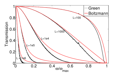
Figure 2: (color online) Averaged transmission function ${\cal T}_{L}(\omega)$ as a function of $\omega$, for different system sizes. From top to down: increasing system sizes from $L=100$ to $L=10^{6}$. The black curves are the transmissions computed with a Green’s function approach, and the red curves are obtained from the Boltzmann formula (19).

The transmission predicted by the Boltzmann approach can be computed analytically in this simple case since there is only a single branch and there are therefore only two conducting states for a given pulsation (due to the symmetry $\omega(k)=\omega(-k)$). It can be shown (see Appendix C) that

$$T_{L}(\omega)=\left(1+\frac{L}{l_{\text{Boltz}}(\omega)}\right)^{-1},$$ (19)

with

$$\frac{1}{\omega^{2}\,l_{\text{Boltz}}(\omega)}=\frac{\text{Var}(m)}{\langle m\rangle^{2}}\left(1-\frac{\omega^{2}}{4}\right)^{-1}.$$

Notice that this expression of the transmission agrees at second order in $\omega$ with (17) in the limit $\omega\to 0$.

The comparison between the transmissions computed with the Green’s function and the Boltzmann approaches shows that the Boltzmann treatment is a reasonable approximation for low frequency modes, but predicts a transmission which is too large for higher frequencies. The critical frequency at which the Boltzmann transmission starts to depart significantly from the Green’s function transmission decreases with the system size. Therefore, we expect the conductances to agree in the low temperature regime for all system lengths, and the relative error to increase with the system length at larger temperatures where the higher frequency part of the transmission are taken into account.

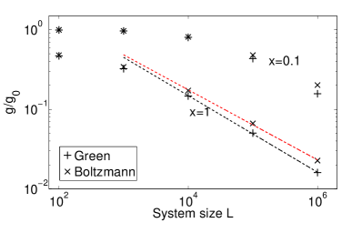
Figure 3: (color online) Conductances computed using the Green’s function approach and a Boltzmann treatment for two values of $x=\hbar\omega/k_{\text{B}}T$. The asymptotic regime where $\overline{g}\sim L^{-\alpha}$ is attained only for $x=1$, with $\alpha\simeq 0.48$ for the Green’s function approach, and $\alpha\simeq 0.44$ in the Boltzmann case.

This is indeed confirmed by the scalings of the normalized thermal conductance in Fig. 3, for different values of $x=\hbar\omega/k_{\text{B}}T$. As expected, the asymptotic scaling $L^{-1/2}$ for the thermal conductance is reached for systems long enough when the transmission is computed using the Green’s function approach. This could be anticipated since the Green’s function results are exact for harmonic systems. On the other hand, the conductances predicted by the Boltzmann approach for systems long enough, are larger than the conductances obtained with the Green’s function approach. The Boltzmann treatment does not predict the right asymptotic scaling either, though the discrepancy is not too large. This is due to the fact that the Boltzmann transmission does not decay fast enough with the system size for larger values of $\omega$.

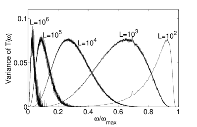
Figure 4: (color online) Top: Transmission computed using the Green’s function technique for a one dimensional chain of length $L=10^{4}$: average transmission (black) and transmission for a single realization of the mass disorder (red). Bottom: Variance of the transmission functions computed using the Green’s function techniques as a function of the pulsation, for different system lengths.

An interesting feature of the transmission function in the one dimensional case is that the maximal variance of ${\cal T}(\omega)$ over the realizations of the transmission computed with different mass disorders does not decrease with the increasing size of the system (though the range of pulsations where the variance is not small decreases). However, the thermal conductance, which is the integral of the transmission function, does not vary much from one realization of the mass disorder to the other. Fig. 4 (Top) presents a plot of a the transmission function for a given realization of the mass disorder, which is compared to the average transmission, while Fig. 4 (Bottom) plots the variance of the transmission as a function of the pulsation. Therefore, it is not true that, when the size of the disordered region increases, all the transmission functions look similar (no thermodynamic limit seems to be reached). There remains some intrinsic variability, which can be used to determine exponential localization lengths.Avriller et al. (2007) This is also reminiscent of the fact that, in molecular dynamics studies of harmonic disordered chains, non smooth steady temperature profiles are obtained when only a single realization of the disorder is considered.Likhachev et al. (2006)

V Numerical results for carbon nanotubes

V.1 Description of the model

We use two distinct models to simulate CNTs. With the first one, labelled as ’ab-initio’ in the sequel, the tube is simulated using the interatomic force constants (IFCs) computed from density functional theory calculations,Baroni et al. (2001) using the PWCSF package of the QUANTUM-ESPRESSO distributionet al. on a (5,5) CNT of experimental (curved) geometry. With the second one, labelled as ’empirical’ in the sequel, the tube is simulated with a flat geometry using the empirical force constants of graphene given in Ref. Saito et al., 1998. The empirical model is used to simulate (5,5) and (10,10) CNTs. In any cases, the models are used consistently within both the Green’s function and Boltzmann approaches. We restrict ourselves to armchair nanotubes for simplicity. Armchair nanotubes are very important for applications since they are metallic (here we compute only the phononic thermal conductance). We expect the results presented below to be robust with respect to the system chirality, because the ballistic conductance does not change much with the chirality.Mingo and Broido (2005a)

In order to have a block tridiagonal form for the interaction matrix within the ab-initio model, only interactions within a cut-off radius $R_{\rm cut}=12$ Bohrs are taken into account. In this case, it is necessary to consider a supercell composed of two elementary cells depicted in Fig. 5 as a unit building block. The projection procedure of Ref. Mounet, 2005 was used to ensure that acoustic sum rules are satisfied for the truncated IFC matrix.

When the empirical model of Ref. Saito et al., 1998 is used, carbon nanotubes are modeled as graphene nanoribbons with periodic boundary conditions in the transverse direction, and interactions up the third neighbors are taken into account. Due to these simplifying assumptions, the in-plane and out-of-plane motions can be computed separately since their contributions are independent. In this case, the elementary cell depicted in Fig. 5 can be chosen as a unit cell. Although less precise (though, as will be shown below, many results are in very good agreeement with the results obtained with the ab-initio based computations), this model is less expensive and was therefore used to study CNTs of larger diameters.

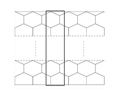
Figure 5: Armchair nanotube, with interactions up the third neighbor. The unit cell of the periodic structure is represented by the box.

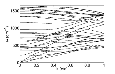
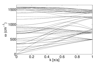
Figure 6: Phonon spectrum of a (5,5) CNT. Top: Ab-initio computed interatomic forces. Bottom: Empirical model described in Section V.1.

We compare in Fig. 6 phonon dispersions for (5,5) armchair tubes obtained with the empirical model and with ab-initio computed IFC. The agreement is fair enough, though the number of acoustic modes is not correct, and the lowest modes do not have a quadratic dispersion relation as is the case for real nanotubes. Despite that, the thermal transport results for both models should agree quantitatively as shown by a comparison of ballistic conductances computed with the empirical model used here and ab-initio reference results.

Actually, a more intrinsic property is the ballistic thermal conductance divided by the cross sectional surface of the material $g/\mathcal{A}$ (this is the so-called ballistic conductivity per unit length, compare with Eq. (12)). The cross sectional area $\mathcal{A}$ is obtained from a “fattened” carbon ring:

$$\mathcal{A}=2\pi Rd=3nd,$$ (20)

where $n$ is the index of the nanotube, $R$ is the radius of the carbon ring and $d=3.35$ Å  (the graphite interlayer separation) is some characteristic length defining the width of the annular domain enclosing the carbon ring. Fig. 7 presents a plot of $g/\mathcal{A}$ as a function of the temperature, for two CNTs of different indices, as well as a reference curve computed from ab-initio results, and experimental results.Yu et al. (2005)

Several conclusions can be drawn from this picture:

1. there is a good agreement between the empirical model used and the reference results computed with ab-initio interatomic force constants on the whole range of temperatures;

2. the agreement with the experimental results from Ref. Yu et al., 2005 for temperatures around room temperature and below, suggests that the present models contain the essentials ingredients for describing thermal transport. In particular, other effects (presently not taken into account) such as anharmonic interactions may be neglected in this temperature regime (and for lower temperatures). The measurements from Ref. Yu et al., 2005 have been transformed into conductivities per unit length by assuming that the CNTs used for the experiments have a diameter of 1 nm. The authors of Ref. Yu et al., 2005 indeed precise that the CNTs used have a diameter in the range 1-2 nm, occasionally 2-3 nm. If the diameter is indeed 1 nm, then the experimental results are close to the ballistic conductance curve, which means that the thermal transport is nearly ballistic.Yu et al. (2005) If the diameters are larger, there is a reduction of about 50% of the conductance for the CNTs of experimental lengths (about $L=2.76~{}\mu$m) with respect to the ballistic conductance. This reduction may be attributed to anharmonic effects. We remark that, even in this case, the effect of isotopic disorder should still be noticeable since the results on the conductivities in Section V.5 show that isotope disorder can lead to a reduction of about 80% of the conductance at room temperature for CNTs of experimental lengths.

In the sequel, results for temperatures much larger than room temperature are also presented. We warn however the reader that these results are given for completeness (having computed the transmission, the thermal conductance can straightforwardly be evaluated at any temperature). It is likely that anharmonic effects become more important as the temperature increases, invalidating the use of a harmonic description in this temperature range.

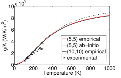
Figure 7: (color online) Ballistic conductivity per unit length (expressed in Å), with the cross sectional area (20) for a (5,5) (red) and a (10,10) (black) nanotube. Experimental points taken from Ref. Yu et al., 2005 are also reported.

Parameters used

The parameters used in this study are given in Table 1 when the empirical model is used. In the case of ab-initio computed IFC, no averaging was performed (since, as shown below in Section V.4, the conductance does not change much from one realization of the mass disorder to another), but the CNTs considered have the same lengths. Since the interatomic distance at equilibrium is $L_{0}\simeq 1.44$ Å, the nanotubes considered have lengths up to $L=2.49$ $\mu$m, which is a length typical of the currently available experimental single walled CNTs. The larger system (i.e. (10,10) CNT of length $L=2.49$ $\mu$m) consists of $400,000$ atoms.

In all this study, $c=0.5$, and the mass disorder corresponds to replacing ¹²C by ¹³C ($\Delta m/m=1/12$). The qualitative features presented are robust with respect to a smaller disorder concentration, but longer tubes should then be studied. Also, the regularizing parameter $\eta/\omega_{\text{max}}^{2}=10^{-8}$.

For ab-initio computed IFC, the transmission is computed for $N_{\omega}=200$ points uniformly spaced in the range $0\leq\omega\leq\omega_{\text{max}}=1650$ cm^-1. For (5,5) CNTs described by the empirical model, $N_{\omega}=1000$ points uniformly spaced in the range $0\leq\omega\leq\omega_{\text{max}}=1650$ cm^-1. For (10,10) CNTs described by the empirical model, the spectral region $0\leq\omega\leq 330$ cm^-1 is discretized using $N_{\omega}=200$ points, while $N_{\omega}=200$ other points are used for the remaining part of the spectrum. Such a decomposition ensures that the low frequency part of the spectrum, which is very important to have reliable estimates of the thermal conductivity, is treated accurately, while keeping the overall computational cost reasonable. The Boltzmann transmissions are computed in all case with $N_{\omega}=1000$.

We studied the dependence on the results on the disorder realization, in the case of CNTs described by the empirical model. For each tube length $L$, $N_{\text{disorder}}$ realizations of the isotopic disorder are considered, and the transmission are averaged over the different realizations. We considered a fixed computational cost for each tube length, so that $LN_{\text{disorder}}$ is constant.

Table 1: Number of averages over the mass disorder realizations as a function of nanotube length for CNTs described by the empirical model.

Length (nm)	2490	823	249	82.3	24.9	8.23
$N_{\text{layers}}$	$10^{4}$	3300	1000	330	100	33
$N_{\text{disorder}}$	1	3	10	30	100	300

V.2 Average transmissions

The average transmission functions are presented in Fig. 8. The different transmission pictures obtained show that the higher frequency modes are damped out first, while the acoustic modes are less perturbed. In general, the transmission decreases with the pulsation. Longer system sizes are necessary to modify substantially the transmission of acoustic modes. As the carbon nanotube index (equivalently, its diameter) increases, the spikes in the transmission become less marked, and the behavior of the transmission as a function of the pulsation is almost monotonic.

Although not shown here, the maximal variance over the transmission functions computed for different realizations of the mass disorder is constant for different tube lengths, as is the case for one-dimensional chains. However, the relative variation of the transmission (defined as the square root of the variance divided by the average transmission) decreases with the CNT index. This is due to the fact that transmission fluctuations remains of order 1, while the ballistic transmission (the number of conducting channels) increases proportionally to the system index.

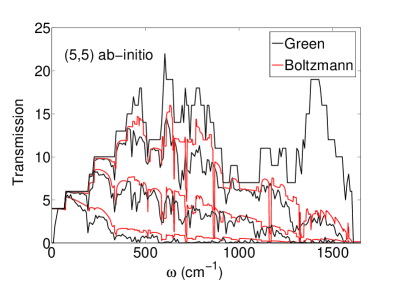
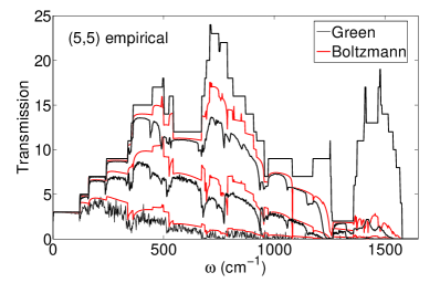
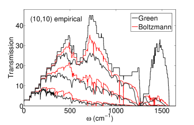
Figure 8: (color online) Transmissions obtained with the Green’s function formalism (black curves) and the Boltzmann approach (red curves). In each of the three figures, the line corresponding to the largest transmission is the reference ballistic transmission. The other lines correspond to tubes of different lengths, namely $L=25$ nm, $L=249$ nm and $L=2.49$ $\mu$m, the highest transmissions corresponding to the shortest tubes.

The Boltzmann transmission is in fair agreement with the Green’s function transmission, especially at low frequencies. At higher frequencies, the Boltzmann transmission is usually higher than the Green’s function one. This is in analogy with the results for the dimensional chains. The largest discrepancies arise however for pulsations in the range $\omega=400-500$ cm^-1, corresponding to the out-of-plane phonon modes. The agreement seems however better when ab-initio IFCs are used. This may be due to the fact that in-plane and out-of-plane modes interact in this case (indeed, the Boltzmann treatment is expected to be more accurate when the number of interacting modes is larger).

V.3 Determination of the transmission regime at some chosen frequencies

Anderson localizationAnderson (1958) is often observed in one-dimensional disordered systems. In this case, the transmission function decreases exponentially with the system size (in average). This is the case for isotopically disordered harmonic one-dimensional chain (see Section IV.1), for which however the localization length goes to infinity when the pulsation goes to 0. When many conducting channels are present in a disordered harmonic system, it is unclear whether the transmission is still localized, or if it becomes closer to a diffusive behavior.

We discuss here whether the transmission regime is diffusive or localized for a given pulsation $\omega$. There are several ways to determine the nature of the transmission regime, see for instance the recent workAvriller et al. (2007) where diffusive and localized lengths for different system sizes are computed. We compute here the diffusive and localized lengths by resorting to some functional ansatz of the transmission function which allows to interpolate between the two regimes. The transmission considered is the average transmission since this is the quantity of interest. The (average) transmission function computed by the Green’s function and the Boltzmann approaches may be approximated by the following ansatz:

$$T^{\text{ansatz}}_{L}(\omega)=T_{\textrm{ballistic}}(\omega)\,\left(1+\frac{L}{l_{\textrm{diff}}(\omega)}\right)^{-1}\text{e}^{-L/l_{\textrm{loc}}(\omega)},$$ (21)

where $l_{\textrm{diff}}(\omega)$ is some characteristic length associated with diffusive transport at the pulsation $\omega$ (inducing a $1/L$ decay) while $l_{\textrm{loc}}(\omega)$ measures the propensity of the system to localize its states (inducing an exponential decay of the transmission as in the Anderson model).

To determine the lengths $l_{\textrm{diff}}(\omega),l_{\textrm{loc}}(\omega)$, we compute $N_{\text{realizations}}$ values of the transmission at a fixed value of $\omega$ for several lengths $L=L_{1},\dots,L_{N_{\text{lengths}}}$, and perform a least-square fit of the average transmission based on the ansatz (21). Many realizations should be considered in order to have reliable results, and so, we restricted ourselves to the simple empirical model; here $N_{\text{realizations}}=300$. Besides, it is actually not always sufficient to perform a least-square fit directly on the transmissions. Indeed, when the transmission regime is (close to) localized, the direct estimates give poor results since the transmission is asymptotically very small, and the corresponding points have very small weights in the direct least-square fitting procedure. Therefore, we resort to a nonlinear least-square fit, where $f(T_{L}(\omega))$ and $f(T_{L}^{\text{ansatz}}(\omega))$ are compared. The function $f$ puts more emphasis on the asymptotic regime, i.e. on the smaller values of the transmission. The choice $f=-\log$ is convenient, but other choices such as $f(x)=1/x$ yielded similar results.

Fig. 9 presents a typical fit in the diffusive regime at the frequency $\omega=716$ cm^-1 for a (10,10) CNT, and compares the normalized transmissions $T_{L}(\omega)/T_{\text{ballistic}}(\omega)$ computed using both Boltzmann and Green’s function methods. As can be seen, the functional form of the ansatz (21) is indeed appropriate.

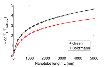
Figure 9: (color online) Fit of $-\ln(T_{L}/T_{\text{ballistic}})$ as a function of $L$ at $\omega=716$ cm^-1 for a (10,10) CNT described by the empirical model. The transmission computed with the Green’s function and Boltzmann methods can be fitted with a good precision using the ansatz (21) (solid black and red lines).

The characteristic lengths as for different pulsations are presented in Table 2 for (5,5) CNTs, and in Table 3 for (10,10) CNTs (for some pulsations, the transmission decreases too fast with increasing system size, and no fitting could be performed). Using these results, it is possible to determine whether the transmission regime is diffusive or localized. Notice however that the diffusive and localized lengths as defined by (21) should not be compared directly when they are of the same order of magnitude. Rather, given some attenuation factor $0\leq\gamma\leq 1$ (typically, $\gamma=0.1$), one should compare the lengths of the sample required to reduce the ballistic transmission by a factor $\gamma$. For the diffusive term, this is $L\sim(1/\gamma-1)l_{\textrm{diff}}(\omega)$, while for the localized regime $L\sim-l_{\textrm{loc}}(\omega)\ln\gamma$.

The results of Tables 2 and 3 show that, for the exact (Green’s function) transmission, the localization length decreases with increasing frequencies, so that localization effects become more and more important as the pulsation increases. This explains the fast decrease of the high frequency modes. The behavior of the diffusive lengths is not as clear cut as the behavior of the localization lengths: the diffusive lengths decrease at smaller pulsations, and then settle down to values around $100-300$ nm, which are therefore completely relevant for CNTs of experimental sizes. It seems that some minimal diffusive length is obtained when the number of channel is maximal, which is consistent with the picture that diffusive transport arises from random scattering between many channels.

For the Boltzmann transmission, only the diffusive part is relevant since the localization lengths computed are always much larger than the diffusive lengths. There is also a trend towards shorter diffusive lengths as the pulsation increases. This may be explained by the fact that the scattering for higher frequencies is much more efficient than for acoustic modes, which, in turn, comes from the $\omega^{2}$ dependence in the expression of the scattering matrix (15).

Finally, it is observed that both diffusive and localization lengths increase with increasing diameter of the system, especially the localization length. This can related again to an increase of the number of available modes with increasing diameters, and thus, a reduced scattering.

Table 2: Localization and diffusive lengths (expressed in nm) for a (5,5) CNT described by the empirical model.

		Green		Boltzmann
$\omega$ (cm-1)	$T_{\text{ballistic}}$	$l_{\textrm{diff}}$	$l_{\textrm{loc}}$	$l_{\textrm{diff}}$	$l_{\textrm{loc}}$
90	3	77100	$7\times 10^{7}$	$1\times 10^{5}$	$1\times 10^{7}$
179	7	3399	$2\times 10^{7}$	5273	456000
269	9	1422	$1\times 10^{11}$	2990	$9\times 10^{10}$
358	13	304	52800	897	$2\times 10^{10}$
448	15	387	$2\times 10^{11}$	779	212000
537	16	239	13700	433	33800
627	12	320	10900	455	28100
716	23	72.9	4897	139	24600
806	18	119	6552	215	27100
896	14	101	4007	180	23900
985	9	149	2502	156	23800
1075	9	117	1716	85	19600
1164	7	341	289	78.2	18300
1254	7	$2\times 10^{6}$	207	2.62	1993
1343	2	$9\times 10^{9}$	39.8	288	25200
1433	13	$2\times 10^{10}$	136	6.35	4392

Table 3: Localization and diffusive lengths (expressed in nm) for a (10,10) CNT described by the empirical model.

		Green		Boltzmann
$\omega$ (cm-1)	$T_{\text{ballistic}}$	$l_{\textrm{diff}}$	$l_{\textrm{loc}}$	$l_{\textrm{diff}}$	$l_{\textrm{loc}}$
179	11	1927	$4\times 10^{10}$	6727	$1\times 10^{6}$
358	25	494	$1\times 10^{12}$	1165	241000
537	30	235	212000	395	31900
716	45	76.5	12500	166	26000
896	26	125	9269	194	24200
1075	15	101	2851	118	21300
1254	13	–	–	3.12	1824
1433	29	114	88.0	5.43	3189

V.4 Asymptotic scaling of the thermal conductance

Before discussing the properties of the thermal conductance, we first check whether the realizations of the mass disorder have a noticeable influence on the value of the normalized thermal conductance $\overline{g}$ given by (11). This is important from an experimental viewpoint since only few (if not only one) realizations of the mass disorder can be considered. Fig. 10 presents the normalized standard deviation of the conductance, for different system sizes, as a function of the temperature. The variations of the conductance are lower than 1% from one realization to the other. This is due to the fact that the conductance is the integral of the transmission function (with the proper weighting function), and therefore the variations of the transmission function for only one realization of the mass disorder are averaged out.

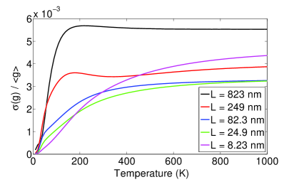
Figure 10: (color online) Standard deviation of the conductance $\sigma(g)$ of a (5,5) CNT (described by the empirical model) divided by average conductance $\langle g\rangle$, as a function of temperature, for different system sizes.

Fig. 11 presents the averaged normalized thermal conductance as a function of the system length (in log-log scale) for (5,5) and (10,10) CNTs. Three temperatures are considered in both cases: $T=50$ K, $T=300$ K, $T=1000$ K. The scalings obtained for $T=50$ K show that the transmission regime is quasi-ballistic since the conductance does not change much with the system size. Indeed, at low temperatures, only the low frequencies modes, which are almost unaffected by the disorder, matter. For higher temperatures, more and more higher frequency modes are introduced, so that disorder has a noticeable effect, and the conductance decreases as a function of the system size. When this makes sense, the slope $\alpha$ of the different curves have been estimated using some least-square fitting, in order to characterize a power law decay $\overline{g}\sim L^{-\alpha}$. The exponents found are in the range $\alpha=0.4-0.5$ at $T=300$ K. The associated thermal conductivities therefore have a power-law divergence $gL/\mathcal{A}\sim L^{\beta}$ with $\beta=1-\alpha=0.5-0.6$ for the range of lengths considered in this study. The general trends in the curves are quite comparable for (5,5) and (10,10) CNTs, independently of the model used.

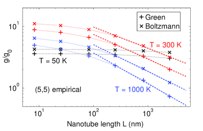
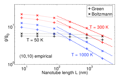
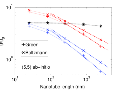
Figure 11: (color online) Variation of the normalized conductance for temperatures $T=50$ K (black curves), $T=300$ K (red curves), $T=1000$ K (blue curves), for the conductivities computed with the Green’s function approach and the conductivities computed with the Boltzmann approach. For a given temperature, the Boltzmann curve is always above the Green’s function curve. Top: (5,5) CNT, estimated $\alpha=0.40$ at $T=300$ K and $\alpha=0.50$ at $T=1000$ K. Middle: (10,10) CNT, estimated $\alpha=0.41$ at $T=300$ K and $\alpha=0.50$ at $T=1000$ K. Bottom: (5,5) CNT with ab-initio IFCs, estimated $\alpha=0.43$ at $T=300$ K and $\alpha=0.55$ at $T=1000$ K.

Notice that the asymptotic regime is not yet attained for nanotubes of lengths up to $2.5~{}\mu$m (which are typical experimental lengths). In this regime the exponent $\alpha$ is not universal since it depends on the tube length and on the amount of mass disorder. As in the case of one dimensional chains, the truly asymptotic regime corresponds to $\overline{g}\sim L^{-1/2}$ (or $\kappa\sim L^{1/2}$), with associated transmission profiles where only acoustic modes have a non-zero transmission. To this end, much larger system sizes (or a larger mass disorder) should be considered. In any cases, it is observed that there is no well-defined conductivity.

V.5 Thermal conductance as a function of the temperature

The temperature dependence of the normalized conductance is presented in Fig. 12. Those curves are obtained for the transmission computed with the Green’s function approach, and the curves for the transmission computed using a Boltzmann treatment have a very similar behavior with respect to temperature. As expected, the ratio of the thermal conductance to the ballistic one is always smaller than 1, and converges to 1 in the low temperature limit.

Several conclusions can be drawn from this picture: (i) the relative reduction of the conductance due to the isotope disorder does not depend on the CNT diameter; (ii) the decrease predicted by Boltzmann equation is in excellent agreement with the decrease found with the Green’s function method; (iii) isotopic disorder can be very efficient in reducing the thermal conductivity, especially for tubes of experimental lengths, even at moderately high temperatures. For instance, for (5,5) and (10,10) tubes of experimental lengths ($L=2.49$ $\mu$m), the thermal conductance is decreased by 80% at room temperature. Notice that the decrease in the thermal conductivity increases with the temperature. This is consistent with the results of the previous sections since, as the temperature is increased, more and more higher frequency modes are introduced, and the transmission function is almost a decreasing function of the pulsation.

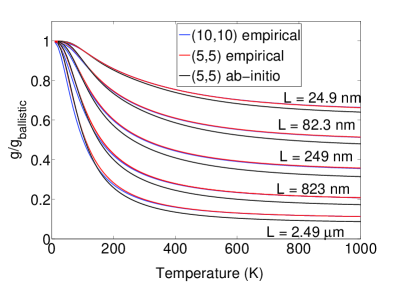
Figure 12: (color online) Ratio of the thermal conductance to the ballistic conductance, for (10,10) empirical CNT (blue curves), (5,5) empirical CNT (red curves) and (5,5) ab-initio CNT (black curves). From top to down: increasing tube lengths.

The thermal conductivity (or conductance) predicted by the Boltzmann approach is compared to the conductivity (or conductance) obtained by the Green’s function approach. The results are presented in Fig. 13, where the error

$$e(T)=\frac{\kappa_{\text{Boltzmann}}-\kappa_{\text{Green}}}{\kappa_{\text{Green}}},$$

is plotted as a function of the temperature $T$. As can be seen, the Boltzmann approach gives correct orders of magnitude in the temperature range and for the CNT index considered here. It however overestimates the conductivity, and the error increases with the length of the system and the temperature. This can be explained by the fact that the Boltzmann approach is not precise enough to capture the real decay of the transmission function. In particular, the decrease of the transmission is not fast enough, which is consistent with the results of Fig. 8.

However, as already pointed out in Section V.2, it is expected that the Boltzmann treatment becomes more accurate as the number of interacting modes increases. It is therefore likely that the agreement between the conductance computed using Green’s function techniques and conductances computed from the Boltzmann transmissions will be better for tubes with larger indices or multi-walled tubes (or for models treating the out-of-plane modes more precisely). This is indeed true, as can be seen from the results presented in Fig. 13, where the error on the conductivity is smaller for CNTs of larger diameters (To give some orders of magnitude, the diameters of (5,5) and (10,10) CNTs are respectively 0.69 nm and 1.38 nm).

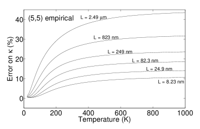
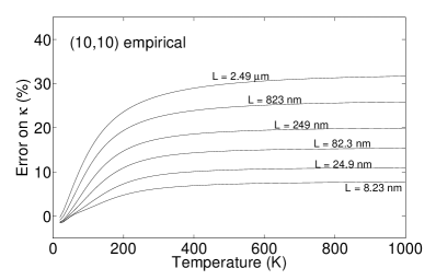
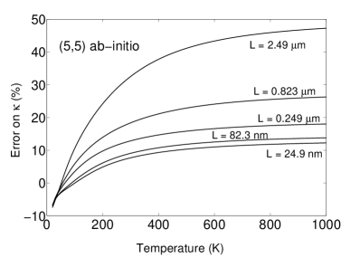
Figure 13: Error on the the conductivity computed with the profile obtained from the Boltzmann approach. The reference value is computed from the profiles obtained with the Green’s function approach (decreasing lengths from top to down).

VI Conclusion

We studied the thermal transport of isotopically disordered harmonic CNTs using Green’s function and Boltzmann treatments. The Green’s function method is implemented using an algorithm, whose computational cost scales linearly with the system size. It is not restricted to isotopic disorder, and can be applied to other kind of defects which scatter phonons elastically.Mingo et al. (2008) In view of the theoretical results for 1D systems, we also expect a divergence of the thermal conductivity with the system size in those cases.

Our numerical results show that

1. these systems share some common features with the thermal transport in isotopically disordered harmonic one dimensional atom chains, in particular a power law divergence of the thermal conductivity $\kappa\sim L^{\alpha}$. Therefore, Fourier’s law is not valid. For tubes of experimental length, the exponent of the power law divergence $\alpha\simeq 0.6$ at room temperature. For longer tubes, the exponent may well be different since $\alpha=1/2$ in the asymptotic regime where only the acoustic branches have a non-zero transmission. Experimental results on the length dependence of disordered CNT conductivities, measuring divergences $\alpha\simeq 0.4-0.6$ for boron nitride tubes (with a large fraction of mass disorder), have been published in Ref. Chang et al., 2008

2. the thermal conductivity decreases monotonically with the temperature, and is independent of the CNT diameter. We showed that there is a dramatic reduction of the thermal conductance for systems of experimental sizes (roughly 80% at room temperature), when a large fraction of isotopic disorder is introduced. This is in accordance with experimental measurements of the effect of isotope disordered in boron nitride nanotubes, which demonstrated dramatic changes in the conductances (a conductance enhancement by 50% for purified materials);Chang et al. (2006)

3. a Boltzmann description of the thermal transport gives correct results for the thermal conductance even in the presence of Anderson localization. This is particularly interesting since the computation of the transmission using Boltzmann’s equation is much less computationally expensive, so that larger systems (such as multi-walled CNTs or boron nitride nanotubes, or single-walled CNTs with a large diameter) may be studied with this method. This shows also that Anderson localization, that is not accounted for in the Boltzmann approach, does not have a clear signature in thermal transport for CNTs of experimental sizes;

4. the results discussed in the previous points are robust with respect to the model used to describe the phonon dispersion in the nanotube. In particular, the behaviors predicted by a simple empirical model which neglects the tube curvature are very similar to those obtained with ab-initio force constants, computed with density functional theory, and considering the tube curvature.

Appendix A Computation of the transmission within the Green’s function formalism

In order to simplify the notations, the number of layers in the disordered region $N_{\text{layers}}$ will be denoted by $N$ in this section. Besides, the parameter $\eta$ is always kept positive in numerical computations. We indicate explicitly the dependence on this parameter in this section.

The $(i,j)$ block component of some matrix $\mathcal{M}$ is denoted by $[\mathcal{M}]_{i,j}$. It is easily seen that the only non zero block components of the self-energies are respectively $[\Sigma_{L}^{\eta}(\omega)]_{1,1}$ and $[\Sigma_{R}^{\eta}(\omega)]_{N,N}$. These coefficients are computed using standard decimation techniques.da Silva and Koiller (1981); Guinea et al. (1983); Lopez-Sancho et al. (1984, 1985)

The transmission ${\cal T}(\omega)$ can be evaluated using only the block $[G^{\eta}_{\text{sys}}(\omega)]_{1,N}$ of the full matrix $G^{\eta}_{\text{sys}}(\omega)$ since

$${\cal T}(\omega)=4\,\textrm{Tr}\left[\textrm{Im}([\Sigma_{L}^{\eta}(\omega)]_{1,1})\,[G_{\textrm{sys}}^{\eta}(\omega)]_{1,N}\,\textrm{Im}([\Sigma_{R}^{\eta}(\omega)]_{N,N})\left([G_{\textrm{sys}}^{\eta}(\omega)]_{1,N}\right)^{\dagger}\right],$$

where the trace is taken over a space of dimension $3N_{\text{at}}\times 3N_{\text{at}}$.

The submatrix $[G^{\eta}_{\text{sys}}(\omega)]_{1,N}$ can be computed by solving

$$G^{\eta}_{\text{sys}}(\omega)^{-1}\left(\begin{array}[]{l}\left[G_{\textrm{sys}}^{\eta}(\omega)\right]_{1,N}\\ \qquad\vdots\\ \left[G_{\textrm{sys}}^{\eta}(\omega)\right]_{N-1,N}\\ \left[G_{\textrm{sys}}^{\eta}(\omega)\right]_{N,N}\\ \end{array}\right)=\left(\begin{array}[]{c}0\\ \vdots\\ 0\\ \textrm{I}\\ \end{array}\right),$$

with

$$G^{\eta}_{\text{sys}}(\omega)^{-1}=\omega^{2}+\text{i}\eta-A_{\rm sys}-\Sigma^{\eta}_{L}(\omega)-\Sigma^{\eta}_{R}(\omega).$$

We use a method to compute linear scalingly the last column of the inverse of a block tridiagonal matrix, based on gaussian elimination. Each $[G_{\textrm{sys}}^{\eta}(\omega)]_{i,N}$ is expressed in terms of $[G_{\textrm{sys}}^{\eta}(\omega)]_{i+1,N}$ as $[G_{\textrm{sys}}^{\eta}(\omega)]_{i,N}=F_{i}[G_{\textrm{sys}}^{\eta}(\omega)]_{i+1,N}$. Denoting by $B=\omega^{2}+\text{i}\eta-A_{\text{sys}}-\Sigma^{\eta}_{L}(\omega)-\Sigma^{\eta}_{R}(\omega)$ and $f_{i}=[G_{\textrm{sys}}^{\eta}(\omega)]_{i,N}$, it holds, for $2\leq i\leq N-1$,

$$B_{i,i-1}f_{i-1}+B_{i,i}f_{i}+B_{i,i+1}f_{i+1}=0,\qquad f_{i}=F_{i}f_{i+1}.$$

It is then easily shown that

$$F_{1}=-B_{1,1}^{-1}B_{1,2},$$

$$F_{i}=-(B_{i,i}+B_{i,i-1}F_{i-1})^{-1}B_{i,i+1}\ \ (2\leq i\leq N-1)$$

while $f_{N}=(B_{N,N}+B_{N,N-1}F_{N-1})^{-1}$, so that $[G^{\eta}_{\text{sys}}(\omega)]_{1,N}=f_{1}=F_{1}F_{2}\dots F_{N-1}f_{N}$ is recovered in $\text{O}(Nd^{3})$ operations. The corresponding algorithm therefore has a cost $\text{O}(N_{\text{layers}}N_{\text{at}}^{3})$ (see Algorithm 1).

Iterative computation of the $(1,N)$ block of the effective resolvent

Algorithm 1.

Fix $\omega^{2}\geq 0$ and $\eta>0$, and denote $B=\omega^{2}+\text{i}\eta-A_{\text{sys}}-\Sigma^{\eta}_{L}(\omega)-\Sigma^{\eta}_{R}(\omega)$. Set $$F_{1}=-B_{1,1}^{-1}B_{1,2},\qquad g=F_{1}.$$ Then,  (1) For $i=2,\dots,N-1$, compute $$F_{i}=-(B_{i,i}+B_{i,i-1}F_{i-1})^{-1}B_{i,i+1},$$ and replace $g$ by $gF_{i}$;  (2) Set $[G^{\eta}_{\text{sys}}(\omega)]_{1,N}=g\,(B_{N,N}+B_{N,N-1}F_{N-1})^{-1}$.

An alternative linear scaling algorithm to compute the transmission is proposed in Ref. Lake et al., 1997. This algorithm also allows to compute the density of states in $\text{O}(N_{\text{layers}}N_{\text{at}}^{3})$ operations, but gives wrong transmissions for non small values of $\eta$ (in the results presented in this work, this occurs for even for values $\eta/\omega_{\text{max}}^{2}=10^{-4}$ for one dimensional chains long enough or when the variance of the mass disorder is large enough).

Appendix B Numerical implementation of the Boltzmann equation

To simplify the notations, we drop the variable $\omega$ in the phonon distributions (since it merely indexes independent Boltzmann equations). To solve (14), it is convenient first to symmetrize the problem by introducing $f_{j,\sigma}=v_{j}n_{j,\sigma}$, so that (14) can be recast as

$$\left(\sigma\partial_{t}+\partial_{x}\right)f_{j,\sigma}(x,t)=\sum_{(j^{\prime},\sigma^{\prime})}A_{(j,\sigma),(j^{\prime},\sigma^{\prime})}\,f_{j^{\prime},\sigma^{\prime}}(x,t),$$ (22)

where the matrix $A$ is symmetric. More precisely,

$$A_{(j,\sigma),(j^{\prime},\sigma^{\prime})}=\sigma\frac{W_{(j,\sigma),(j^{\prime},\sigma^{\prime})}}{v_{j}v_{j^{\prime}}}$$

when $(j^{\prime},\sigma^{\prime})\not=(j,\sigma)$ and

$$A_{(j,\sigma),(j,\sigma)}=-\sigma\sum_{(j^{\prime},\sigma^{\prime})\not=(j,\sigma)}\frac{W_{(j,\sigma),(j^{\prime},\sigma^{\prime})}}{v_{j}\,v_{j^{\prime}}}.$$

The boundary conditions for (22) are obtained from the boundary conditions for (14):

$$f_{j,+}(0,t)=v_{j},\qquad f_{j,-}(L,t)=0.$$

We denote $f=(f_{1,+},\dots,f_{N,+},f_{1,-},\dots,f_{N,-})$. Recall that $2N$ is the number of conducting channels at this pulsation. The stationary solution of (22) is such that $f(x)=\exp(xA)\,f(0)$, and thus $f(0)=\exp(-LA)\,f(L)$, where we dropped the argument $t$. This expression has a meaning since $A$ is real symmetric hence defines a self-adjoint operator. Expressing $\exp(-LA)$ as a $2\times 2$ matrix where the entries are $N\times N$ matrices:

$$\exp(-LA)=\left(\begin{array}[]{cc}B_{11}(L)&B_{12}(L)\\ B_{21}(L)&B_{22}(L)\\ \end{array}\right),$$

it holds $B_{11}(L)\cdot(f_{1,+}(L),\dots,f_{N,+}(L))^{t}=(v_{1},\dots,v_{N})^{t}$. Defining the $N\times N$ matrix ${\cal B}(L)=B_{11}^{-1}(L)$ when this inverse exists, the transmission is finally

$$T=N\frac{\displaystyle\sum_{i=1}^{N}f_{i,+}(L)}{\displaystyle\sum_{i=1}^{N}v_{i}}=N\frac{\displaystyle\sum_{i=1}^{N}\sum_{j=1}^{N}{\cal B}_{ij}(L)v_{j}}{\displaystyle\sum_{i=1}^{N}v_{i}}.$$

In practice, it is not possible to use this formula, since the matrix $B_{11}(L)$ becomes singular when $L$ is large. In those cases, we compute a stationary solution of the Boltzmann equation (22) by integrating in time the corresponding partial differential equation (PDE). The discretization is done on a reference geometry (thanks to the hyperbolic scaling of the transport part, it is possible to map a system of size $L$ to a system of size unity, upon rescaling time and the scattering terms by a factor $L$). The numerical scheme uses a splitting of the dynamics into a transport part (which is implemented with a simple upwind schemeGodlewski and Raviart (1996) since the sign of the velocities are known and are constant), and a collisional part (which is integrated exactly using a matrix exponential). The stability conditions on the time step (the so-called CFL conditions in the literature on systems of conservation lawsGodlewski and Raviart (1996)) arise therefore only from the transport part of the equation, and are easy to state since the geometry is kept fixed. We have checked that the algebraic method using the inversion of matrix exponentials and the computation of the steady state through the time integration of the PDE give the same results when the condition number of the matrix $B_{11}$ is not too large. Another consistency check is the fact that the computed transmission is almost constant in space (up to the convergence error).

In the simulation results presented in this work, we have used $N_{x}=200$ discretization points on the reference interval $[0,1]$, and a time step $\Delta t=1.25\times 10^{-3}$ for the time integration of (22). We have checked the convergence of the results with respect to $N_{x}$ and $\Delta t$.

The scattering matrices (15) have been obtained by considering a discrete phonon spectrum computed with $10^{4}$ $k$-points in the first Brillouin zone, and by using windows of width $3.2$ cm^-1 centered around the pulsations $\omega$ of interest to list all the branches at this pulsation. An approximation of the phonon velocity is obtained through finite differences. Some scattering matrices are discarded in the end when they contain too large values (which happens when the velocity of a branch vanishes). This represents less than 1% of the cases for the profiles computed. Such a procedure cannot however be used when the CNT index increases since more and more branches start with a slope zero, and refined strategies should then be employed for larger systems.

Appendix C Derivation of the Boltzmann formula (19)

For one dimensional chains, there is a single conducting branch parametrized by $k$ in the first Brillouin zone:

$$\omega(k)^{2}=2(1-\cos(ka)),\qquad-\frac{\pi}{a}\leq k<\frac{\pi}{a},$$ (23)

where $a$ denotes the lattice spacing in this appendix (In section IV, $a=1$). The steady-state Boltzmann equation at some frequency $\omega$ reduces to

$$\partial_{x}n_{+}(x)=\frac{n_{-}(x)-n_{+}(x)}{l},$$

$$-\partial_{x}n_{-}(x)=\frac{n_{+}(x)-n_{-}(x)}{l},$$

where the dependence on $\omega$ is not written out explicitly, and

$$l^{-1}\equiv l(\omega)^{-1}=\frac{W_{+,-}(\omega)}{v^{2}(\omega)}=a\frac{\text{Var}(m)}{\langle m\rangle^{2}}\frac{\omega^{2}(k)}{\omega^{\prime}(k)^{2}}.$$

From (23), $\partial_{x}(n_{+}-n_{-})=0$. Using the boundary conditions $n_{+}(0)=1$, $n_{-}(L)=0$, and denoting by $n_{+}(L)=T$ and $n_{-}(0)=R$ the proportions of transmitted and reflected waves respectively, it follows $(n_{+}-n_{-})(x)=(n_{+}-n_{-})(0)=(n_{+}-n_{-})(L)=T$. Plugging this result in (23),

$$\partial_{x}n_{+}(x)=-\frac{T}{l},$$

so that

$$n_{+}(x)=1-\frac{x}{l}T.$$

The transmission is then computed at $x=L$ using the above expression for $n_{+}$:

$$T_{L}(\omega)=\frac{l(\omega)}{l(\omega)+L}.$$

To obtain (19), it remains to precise the value of $l^{-1}\equiv l(\omega)^{-1}$. From (23), the phonon velocity is

$$\omega^{\prime}(k)=\frac{a\sin(ka)}{\omega},$$

so that the result follows using $\sin(ka)^{2}=1-\cos(ka)^{2}=1-(1-\omega^{2}/2)^{2}=\omega^{2}(1-\omega^{2}/4)$.

References

- Yu et al. (2005) C. Yu, L. Shi, Z. Yao, D. Li, and A. Majumdar, Nano Lett. 5, 1842 (2005).
- Hone et al. (1999) J. Hone, M. Whitney, C. Piskoti, and A. Zettl, Phys. Rev. B 59, R2514 (1999).
- Yamamoto et al. (2007) T. Yamamoto, Y. Nakazawa, and K. Watanabe, New J. Phys. 9, 245 (2007).
- Rieder et al. (1967) Z. Rieder, J. Lebowitz, and E. Lieb, J. Math. Phys. 8, 1073 (1967).
- Wang et al. (2007) Z. Wang, D. Tang, X. Zheng, W. Zhang, and Y. Zhu, Nanotechnology 18, 475714 (2007).
- Chang et al. (2008) C. W. Chang, D. Okawa, H. Garcia, A. Majumdar, and A. Zettl, Phys. Rev. Lett. 101, 075903 (2008).
- Pop et al. (2006) E. Pop, D. Mann, Q. Wang, K. Goodson, and H. Dai, Nano Lett. 6, 96 (2006).
- Simon et al. (2005) F. Simon, C. Kramberger, R. Pfeiffer, H. Kuzmany, V. Zolyomi, J. Kurti, P. Singer, and H. Alloul, Phys. Rev. Lett. 95, 017401 (2005).
- Chang et al. (2006) C. Chang, A. Fennimore, A. Afanasiev, D. Okawa, I. Ikuno, H. Garcia, D. Li, A. Majumdar, and A. Zettl, Phys. Rev. Lett. 97, 085901 (2006).
- Matsuda and Ishii (1970) H. Matsuda and K. Ishii, Suppl. Prog. Theor. Phys. 45, 56 (1970).
- Bonetto et al. (2000) F. Bonetto, J. Lebowitz, and L. Rey-Bellet, in Mathematical Physics 2000, edited by A. Fokas, A. Grigoryan, T. Kibble, and B. Zegarlinsky (Imperial College Press, 2000), pp. 128–151.
- Lepri et al. (2003a) S. Lepri, R. Livi, and A. Politi, Phys. Rep. 377, 1 (2003a).
- Basile et al. (2006) G. Basile, C. Bernardin, and S. Olla, Phys. Rev. Lett. 96, 204303 (2006).
- Bolsterli et al. (1970) M. Bolsterli, M. Rich, and W. Visscher, Phys. Rev. A 1, 1086 (1970).
- Bonetto et al. (2004) F. Bonetto, J. Lebowitz, and J. Lukkarinen, J. Stat. Phys. 116, 783 (2004).
- Narayan and Ramaswamy (2002) O. Narayan and S. Ramaswamy, Phys. Rev. Lett. 89, 200601 (2002).
- Lepri et al. (2003b) S. Lepri, R. Livi, and A. Politi, Phys. Rev. E 68, 067102 (2003b).
- Mai et al. (2007) T. Mai, A. Dhar, and O. Narayan, Phys. Rev. Lett. 98, 184301 (2007).
- Dhar (2001) A. Dhar, Phys. Rev. Lett. 86, 5882 (2001).
- Yamamoto and Watanabe (2006) T. Yamamoto and K. Watanabe, Phys. Rev. Lett. 96, 255503 (2006).
- Evans (1982) D. Evans, Phys. Lett. A 91, 457 (1982).
- Yao et al. (2005) Z. Yao, J. Wang, B. Li, and G. Liu, Phys. Rev. B 71, 085417 (2005).
- Mingo and Broido (2005a) N. Mingo and D. Broido, Phys. Rev. Lett. 95, 096105 (2005a).
- Lukes and Zhong (2007) J. Lukes and H. Zhong, J. Heat Transfer 129, 705 (2007).
- Maruyama et al. (2006) S. Maruyama, Y. Igarashi, Y. Taniguchi, and J. Shiomi, Journal of thermal science and technology 1, 138 (2006).
- Maruyama (2002) S. Maruyama, Physica B 323, 193 (2002).
- Zhang and Li (2005) G. Zhang and B. W. Li, J. Chem. Phys. 123, 114714 (2005).
- Pan et al. (2007) R. Pan, Z. Xu, and Z. Zhu, Chinese Phys. Lett. 24, 1321 (2007).
- Shiomi and Maruyama (2006) J. Shiomi and S. Maruyama, Phys. Rev. B 74, 155401 (2006).
- Bi et al. (2006) K. Bi, Y. Chen, J. Yang, Y. Wang, and M. Chen, Phys. Lett. A 350, 150 (2006).
- Shenogin et al. (2004) S. Shenogin, A. Bodapati, L. Xue, R. Ozisik, and P. Keblinski, Appl. Phys. Lett. 85, 2229 (2004).
- Zhang et al. (2007) W. Zhang, T. Fisher, and N. Mingo, Numer. Heat Tr. B - Fund. 51, 333 (2007).
- Datta (2005) S. Datta, Quantum Transport: From Atom to Transistor (Cambridge University Press, 2005).
- Datta (2000) S. Datta, Superlattices and microsctructures 28, 253 (2000).
- Ford et al. (1965) G. Ford, M. Kac, and P. Mazur, J. Math. Phys. 6, 504 (1965).
- Dhar and Roy (2006) A. Dhar and D. Roy, J. Stat. Phys. 125, 805 (2006).
- Aschbacher et al. (2007) W. Aschbacher, V. Jaksic, Y. Pautrat, and C.-A. Pillet, J. Math. Phys. 48, 032101 (2007).
- Ashcroft and Mermin (1976) N. Ashcroft and N. Mermin, Solid State Physics (Saunders College Publishing, 1976).
- Baroni et al. (2001) S. Baroni, S. de Gironcoli, and A. D. Corso, Rev. Mod. Phys. 73, 515 (2001).
- Jaksic (2006) V. Jaksic, Lecture Notes in Mathematics 1880, 235 (2006).
- Rego and Kirczenow (1998) L. Rego and G. Kirczenow, Phys. Rev. Lett. 81, 232 (1998).
- Schwab et al. (2000) K. Schwab, E. Henriksen, J. Worlock, and M. Roukes, Nature 404, 974 (2000).
- Mingo and Broido (2005b) N. Mingo and D. Broido, Nano Lett. 5, 1221 (2005b).
- Spohn (2006) H. Spohn, J. Stat. Phys. 124, 1041 (2006).
- Lukkarinen and Spohn (2007) J. Lukkarinen and H. Spohn, Arch. Rational Mech. Anal. 183, 93 (2007).
- Tamura (1983) S. Tamura, Phys. Rev. B 27, 858 (1983).
- Widulle et al. (2002) F. Widulle, J. Serrano, and M. Cardona, Phys. Rev. B 65, 075206 (2002).
- Vandecasteel et al. (2008) N. Vandecasteel, M. Lazzeri, and F. Mauri, unpublished (2008).
- Rubin and Greer (1971) R. Rubin and W. Greer, J. Math. Phys. 12, 1686 (1971).
- Casher and Lebowitz (1971) A. Casher and J. Lebowitz, J. Math. Phys. 12, 1701 (1971).
- Ishii (1973) K. Ishii, Suppl. Prog. Theor. Phys. 45, 77 (1973).
- O’Connor and Lebowitz (1974) A. O’Connor and J. Lebowitz, J. Math. Phys. 15, 692 (1974).
- Keller et al. (1978) J. Keller, G. Papanicolaou, and J. Weilenmann, Commmun. Pure Appl. Math. 32, 583 (1978).
- Rubin (1968) R. Rubin, J. Math. Phys. 9, 2252 (1968).
- Furstenberg (1963) H. Furstenberg, Trans. Am. Math. Soc. 108, 377 (1963).
- Economou (2006) E. Economou, Green’s Function Methods in Quantum Physics (3rd Ed.) (Springer, 2006).
- Avriller et al. (2007) R. Avriller, S. Roche, F. Triozon, X. Blase, and S. Latil, Modern Physics Letters B 21, 1955 (2007).
- Likhachev et al. (2006) V. Likhachev, G. Vinogradov, T. Astakhova, and A. Yakovenko, Phys. Rev. B 73, 016701 (2006).
- (59) S. B. et al., http://www.quantum-espresso.org (????).
- Saito et al. (1998) R. Saito, M. Dresselhaus, and G. Dresselhaus, Physical properties of carbon nanotubes (Imperial College Press, 1998).
- Mounet (2005) N. Mounet, Structural, vibrational and thermodynamic properties of carbon allotropes from first-principles: diamond, graphite, and nanotubes (Master Thesis, MIT, 2005).
- Anderson (1958) P. Anderson, Phys. Rev. 109, 1492 (1958).
- Mingo et al. (2008) N. Mingo, D. A. Stewart, D. A. Broido, and D. Srivastava, Phys. Rev. B 77, 033418 (2008).
- da Silva and Koiller (1981) C. G. da Silva and B. Koiller, Solid State Commun. 40, 215 (1981).
- Guinea et al. (1983) F. Guinea, C. Tejedor, F. Flores, and E. Louis, Phys. Rev. B 28, 4397 (1983).
- Lopez-Sancho et al. (1984) M. Lopez-Sancho, J. Lopez-Sancho, and J. Rubio, J. Phys. F: Met. Phys. 14, 1205 (1984).
- Lopez-Sancho et al. (1985) M. Lopez-Sancho, J. Lopez-Sancho, and J. Rubio, J. Phys. F: Met. Phys. 15, 851 (1985).
- Lake et al. (1997) R. Lake, G. Klimeck, R. Bowen, and D. Jovanovic, J. Appl. Phys. 81, 7845 (1997).
- Godlewski and Raviart (1996) E. Godlewski and P.-A. Raviart, Numerical approximation of hyperbolic systems of conservation laws, vol. 118 of Applied mathematical sciences (Springer-Verlag, 1996).
- Ceperley and Alder (1980) D. M. Ceperley and B. J. Alder, Phys. Rev. Lett. 45, 566 (1980).
- Troullier and Martins (1991) N. Troullier and J. L. Martins, Phys. Rev. B 43, 1993 (1991).
- Fuchs and Scheffler (1999) M. Fuchs and M. Scheffler, Comput. Phys. Commun. 119, 67 (1999).