The problem of analytical calculation of barrier crossing characteristics for Lévy flights

Abstract

By using the backward fractional Fokker-Planck equation we investigate the barrier crossing event in the presence of Lévy noise. After shortly review recent results obtained with different approaches on the time characteristics of the barrier crossing, we derive a general differential equation useful to calculate the nonlinear relaxation time. We obtain analytically the nonlinear relaxation time for free Lévy flights and a closed expression in quadrature of the same characteristics for cubic potential.

1 Introduction

Lévy flights are stochastic processes characterized by the occurrence of extremely long jumps, so that their trajectories are not continuous anymore. The length of these jumps is distributed according to a Lévy stable statistics with a power law tail and divergence of the second moment. This peculiar property strongly contradicts the ordinary Brownian motion, for which all the moments of the particle coordinate are finite. The presence of anomalous diffusion can be explained as a deviation of the real statistics of fluctuations from the Gaussian law, giving rise to the generalization of the Central Limit Theorem by Lévy and Gnedenko [1, 2]. The divergence of the Lévy flights variance poses some problems as regards to the physical meaning of these processes. However, recently the relevance of the Lévy motion appeared in many physical, natural and social complex systems. The Lévy type statistics, in fact, is observed in various scientific areas, where scale invariance phenomena take place or can be suspected (see [3]-[6] and references therein). Lévy flights are a special class of Markovian processes, therefore the Markovian analysis can be used to derive the generalized Kolmogorov equation directly from Langevin equation with Lévy noise [7].

The problem of escape from a metastable state, first investigated by Kramers [8], is ubiquitous in almost all scientific areas (see, for example the reviews [9, 10] and Ref. [11]). Since many stochastic processes do not obey the Central Limit Theorem, the corresponding Kramers escape behavior will differ. An interesting example is given by the $\alpha$-stable noise-induced barrier crossing in long paleoclimatic time series [12]. Another new application is the escape from traps in optical or plasma systems [13]. The main tool to investigate the barrier crossing problem remains the first passage times technique. But for anomalous diffusion in the form of Lévy flights this procedure meets with some difficulties. First of all, the fractional Fokker-Planck equation describing the Lévy flights is integro-differential, and the conditions at absorbing and reflecting boundaries differ from those using for ordinary diffusion. Lévy flights are characterized by the presence of long jumps, and, as a result, a particle can reach instantaneously a boundary from arbitrary position. One can mention some erroneous results obtained in [14] (see also the related correspondence [15]), because author used the traditional conditions at two absorbing boundaries. There are a lot of numerical results regarding the different time characteristics of Lévy flights, but obtaining the exact analytical results remains an open problem (see Ref. [3]).

In this work, starting from the backward fractional Fokker-Planck equation we investigate the barrier crossing event in the presence of Lévy noise, by focusing on the nonlinear relaxation time. The paper is organized as follows. In the following section we shortly review some recent results on barrier crossing problems with different approaches. In section $3.1$, the generalized equations useful to calculate the nonlinear relaxation time (NRLT) are derived. In section $3.2$ we give the exact expressions of NRLT for free Lévy flights and for a cubic potential profile. Finally we draw the conclusions.

2 Barrier crossing

The particle escape from a metastable state, and the first passage time probability density have been recently analyzed for Lévy flights in Refs. [3, 12], [16]- [26]. The main focus in these papers is to understand how the barrier crossing behavior, according to the Kramers law [8], is modified by the presence of the Lévy noise. Here we discuss briefly some results on the barrier crossing events with Lévy flights, recently obtained with different approaches.

The main tools to investigate the barrier crossing problem for Lévy flights are the first passage times, crossing times, arrival times and residence times. We should emphasize that the problem of mean first passage time (MFPT) meets with some difficulties because free Lévy flights represent a special class of discontinuous Markovian processes with infinite mean squared displacement. As already mentioned, the anomalous diffusion in the form of Lévy flights, for a particle moving in a potential profile $U(x)$, is described by the fractional Fokker-Planck equation [6] for the probability density function $W(x,t)$

$$\frac{\partial W}{\partial t}=\frac{\partial}{\partial x}\left[U^{\prime}\left(x\right)W\right]+D\frac{\partial^{\alpha}W}{\partial\left|x\right|^{\alpha}}$$ (1)

where the Riesz fractional derivative is defined as

$$\frac{\partial^{\alpha}f(x)}{\partial|x|^{\alpha}} = \frac{1}{K(\alpha)}\int_{-\infty}^{+\infty}\frac{f(\xi)-f(x)}{|x-\xi|^{1+\alpha}}d\xi$$ (2)

$$= \frac{1}{K(\alpha)}\int_{0}^{+\infty}\frac{f(x+\xi)+f(x-\xi)-2f(x)}{\xi^{1+\alpha}}d\xi.$$

and

$$K\left(\alpha\right)=\frac{\pi}{\Gamma(\alpha+1)\sin{(\pi\alpha/2)}}\,,$$ (3)

with $\Gamma(z)$ the gamma function and $0<\alpha<2$. Due to the integro-differential nature of the equation (1), we cannot apply the usual boundary conditions at the reflecting and absorbing barriers of the system investigated. The particle, in fact, can reach instantaneously the boundaries from any position.

The numerical results for the first passage time of free Lévy flights confined in a finite interval were presented in Ref. [3]. There, the complexity of the first passage time statistics (mean first passage time and cumulative first passage time distribution) was elucidated together with a discussion of the proper setup of corresponding boundary conditions, that correctly yield the statistics of first passages for these non-Gaussian noises. In particular, it has been demonstrated by numerical studies that the use of the local boundary condition of vanishing probability flux in the case of reflection, and vanishing probability in the case of absorbtion, valid for normal Brownian motion, no longer apply for Lévy flights. This in turn requires the use of nonlocal boundary conditions. Dybiec with co-authors found a nonmonotonic behavior of the MFPT as a function of the Lévy index $\alpha$ for two absorbing boundaries, with the maximum being assumed for $\alpha=1$, in contrast with a monotonic increase for reflecting and absorbing boundaries.

According to the Kramers law, the probability distribution of the escape times from a potential well with the barrier of height $U_{0}$, has the exponential form

$$p\left(t\right)=\frac{1}{T_{c}}\exp\left\{-\frac{t}{T_{c}}\right\}$$ (4)

with mean crossing time

$$T_{c}=C\exp\left\{\frac{U_{0}}{D}\right\},$$ (5)

where $C$ is some positive prefactor and $D$ is the noise intensity. The barrier crossing behavior of the classical Kramers problem was investigated, both numerically and analytically, in Refs. [3], [19]- [21], where the role of the stable nature of Lévy flight processes on the barrier crossing event was analyzed. Authors considered Lévy flights in a bistable potential $U\left(x\right)$ by numerical solution of the Langevin equation associated to the fractional Fokker-Planck equation (1)

$$\dot{x}=-U^{\prime}\left(x\right)+\xi^{(\alpha)}\left(t\right)\,,$$ (6)

where $\xi^{(\alpha)}\left(t\right)$ is the symmetric Lévy $\alpha$-stable noise. It was shown that although the survival probability decays again exponentially as in Eq. (4), the mean escape time $T_{c}$ has a power-law dependence on the noise intensity $D$

$$T_{c}\simeq\frac{C(\alpha)}{D^{\mu(\alpha)}}\,,$$ (7)

where the prefactor $C$ and the exponent $\mu$ depend on the Lévy index $\alpha$. Using the Fourier transform of the Eq. (1)

$$\frac{\partial\tilde{W}}{\partial t}=-ikU^{\prime}\left(-i\frac{\partial}{\partial k}\right)\tilde{W}-D\left|k\right|^{\alpha}\tilde{W}\,,$$ (8)

the authors derived the mean escape rate for large values of $1/D$ in the case of Cauchy stable noise $\left(\alpha=1\right)$ in the framework of the constant flux approximation across the barrier. The probability law and the mean value of the escape time from a potential well for all values of the Lévy index $\alpha\in(0,2)$, in the limit of small Lévy driving noise, were also determined in the paper [24] by purely probabilistic methods. The escape times have the same exponential distribution (4). The mean value depends on the noise intensity $D$, in accordance with Eq. (7) with $\mu(\alpha)=1$, and the pre-factor $C$ depends on $\alpha$ and the distance between the local extrema of the potential.

The barrier crossing of a particle driven by symmetric Lévy noise of index $\alpha$ and intensity $D$ for three different generic types of potentials was numerically investigated in Ref. [21]. Specifically: (i) a bistable potential, (ii) a metastable potential, and (iii) a truncated harmonic potential, were considered. For the low noise intensity regime, the result of Eq. (7) was recovered. As it was shown, the exponent $\mu(\alpha)$ remains approximately constant, $\mu\approx 1$ for $0<\alpha<2$; at $\alpha=2$ the power-law form of $T_{c}$ changes into the exponential dependence (5). It exhibits a divergence-like behavior as $\alpha$ approaches $2$. In this regime a monotonous increase of the escape time $T_{c}$ with increasing $\alpha$ (keeping the noise intensity $D$ constant) was observed. For low noise intensities the escape time process corresponds to the barrier crossing by multiple Lévy steps. For high noise intensities, the average escape time curves collapse into a single curve, for all values of $\alpha$. At intermediate noise intensities, the escape time exhibits non-monotonic dependence on the index $\alpha$, while still retains the exponential form of the escape time density.

The first arrival time is an appropriate parameter to analyze the barrier crossing problem for Lévy flights. If we insert in fractional Fokker-Planck equation (1) a $\delta$-sink of strength $q\left(t\right)$ in the origin we obtain the following equation for the non-normalized probability density function $W\left(x,t\right)$

$$\frac{\partial W}{\partial t}=\frac{\partial}{\partial x}\left[U^{\prime}\left(x\right)W\right]+D\frac{\partial^{\alpha}W}{\partial\left|x\right|^{\alpha}}-q\left(t\right)\delta\left(x\right),$$ (9)

from which by integration over all space we may define the quantity

$$q\left(t\right)=-\frac{d}{dt}\int_{-\infty}^{+\infty}W\left(x,t\right)dx,$$ (10)

which is the negative time derivative of the survival probability. According to definition (10), $q\left(t\right)$ represents the probability density function of the first arrival time: once a random walker arrives at the sink it is annihilated. As it was shown in the paper [19] for free Lévy flights $\left(U\left(x\right)=0\right)$, the first arrival time distribution has a heavy tail

$$q\left(t\right)\sim t^{1/\alpha-2}$$ (11)

with exponent depending on Lévy index $\alpha$ $\left(1<\alpha<2\right)$ and differing from universal Sparre Andersen result [27, 28] for the probability density function of first passage time for arbitrary Markovian process

$$p\left(t\right)\sim t^{-3/2}.$$ (12)

In the Gaussian case $\left(\alpha=2\right)$, the quantity (11) is equivalent to the first passage time probability density (12). From a random walk perspective, this is due to the fact that individual steps are of the same increment, and the jump length statistics therefore ensures that the walker cannot hop across the sink in a long jump without actually hitting the sink and being absorbed. This behavior becomes drastically different for Lévy jump length statistics: there, the particle can easily cross the sink in a long jump. Thus, before eventually being absorbed, it can pass by the sink location numerous times, and therefore the statistics of the first arrival will be different from that of the first passage. The result (12) for Lévy flights was also confirmed numerically in the paper [26].

3 Nonlinear relaxation time with Lévy flights

3.1 General equations

The nonlinear relaxation time technique is more suitable for analytical investigations of Lévy flights temporal characteristics, because does not request a constraint on the boundary conditions. According to definition, the nonlinear relaxation time (NLRT) reads

$$T\left(x_{0}\right)=\frac{\int_{0}^{\infty}\left[P\left(t,x_{0}\right)-P\left(\infty,x_{0}\right)\right]dt}{P\left(0,x_{0}\right)-P\left(\infty,x_{0}\right)},$$ (13)

where $P\left(\infty,x_{0}\right)=\lim\limits_{t\rightarrow\infty}P\left(t,x_{0}\right)$ and

$$P\left(t,x_{0}\right)=\int_{L_{1}}^{L_{2}}W\left(\left.x,t\right|x_{0},0\right)dx$$ (14)

represents the probability to find a particle in the interval $\left(L_{1},L_{2}\right)$ at the time $t$, if it starts from point $x=x_{0}$. Let us use the same procedure as for calculating the first passage time probability density (see [29]). If the random process $x\left(t\right)$ is Markovian, the probability density of transitions obeys the following backward Kolmogorov’s equation [30]

$$\frac{\partial W\left(\left.x,t\right|x_{0},0\right)}{\partial t}=\hat{L}^{+}\left(x_{0}\right)W\left(\left.x,t\right|x_{0},0\right)$$ (15)

with the initial condition

$$W\left(\left.x,0\right|x_{0},0\right)=\delta\left(x-x_{0}\right).$$ (16)

Here $\hat{L}^{+}\left(x_{0}\right)$ is the adjoint kinetic operator. After integration with respect to $x$ from $L_{1}$ to $L_{2}$ directly in Eq. (15) and taking into account Eq. (14) we arrive at

$$\frac{\partial P\left(t,x_{0}\right)}{\partial t}=\hat{L}^{+}\left(x_{0}\right)P\left(t,x_{0}\right).$$ (17)

The Eq. (17) should be solved with the initial condition following from Eq. (16)

$$P\left(0,x_{0}\right)=1_{\left(L_{1},L_{2}\right)}\left(x_{0}\right),$$ (18)

where $1_{\left(L_{1},L_{2}\right)}\left(x\right)$ is indicator of the set $\left(L_{1},L_{2}\right)$.

According to Eq. (17) $\hat{L}^{+}\left(x_{0}\right)P\left(\infty,x_{0}\right)=0$, and after integration of this equation with respect to $t$ from $0$ to $\infty$ we obtain (see Eq. (18))

$$\hat{L}^{+}\left(x_{0}\right)Q\left(x_{0}\right)=P\left(\infty,x_{0}\right)-1_{\left(L_{1},L_{2}\right)}\left(x_{0}\right),$$ (19)

where $Q\left(x_{0}\right)$ is the numerator of the expression (13), i.e.

$$Q\left(x_{0}\right)=\int_{0}^{\infty}\left[P\left(t,x_{0}\right)-P\left(\infty,x_{0}\right)\right]dt.$$ (20)

Finally, in accordance with Eqs. (13) and (20) the nonlinear relaxation time can be calculated as

$$T\left(x_{0}\right)=\frac{Q\left(x_{0}\right)}{1-P\left(\infty,x_{0}\right)}\,.$$ (21)

with $x_{0}\in(L_{1},L_{2})$. Although Eqs. (19) and (21) are a useful tool to analyze the temporal characteristics of Lévy flights in different potential profiles $U\left(x\right)$, obtaining the exact analytical results for the generic $\alpha$ parameter, characterizing the anomalous diffusion, is one of the unsolved problems in this research area. Even for some particular potential profile, like the cubic one, to derive a general expression of the NLRT as a function of the Lévy index $\alpha$ is a non trivial problem. In the next section we derive a general differential equation useful to calculate the NLRT for arbitrary Lévy index and we find a closed expression for the case of Cauchy stable noise excitation $(\alpha=1)$.

3.2 Lévy flights in a cubic potential

The forward fractional Fokker-Planck equation for Lévy flights in the potential profile $U\left(x\right)$ reads

$$\frac{\partial W\left(\left.x,t\right|x_{0},0\right)}{\partial t}=\frac{\partial}{\partial x}\left[U^{\prime}\left(x\right)W\left(\left.x,t\right|x_{0},0\right)\right]+D\frac{\partial^{\alpha}W\left(\left.x,t\right|x_{0},0\right)}{\partial\left|x\right|^{\alpha}},$$ (22)

where $0<\alpha<2$. It is easily to find from Eq. (22) the expression for the adjoint kinetic operator

$$\hat{L}^{+}\left(x_{0}\right)=-U^{\prime}\left(x_{0}\right)\frac{\partial}{\partial x_{0}}+D\frac{\partial^{\alpha}}{\partial\left|x_{0}\right|^{\alpha}}.$$ (23)

Substituting Eq. (23) in Eq. (19) we arrive at

$$D\frac{d^{\alpha}Q\left(x_{0}\right)}{d\left|x_{0}\right|^{\alpha}}-U^{\prime}\left(x_{0}\right)\frac{dQ\left(x_{0}\right)}{dx_{0}}=P\left(\infty\right)-1_{\left(L_{1},L_{2}\right)}\left(x_{0}\right),$$ (24)

because the probability $P\left(\infty,x_{0}\right)$ does not depend on the initial position of the particles.

The Fourier transform of Eq. (24) gives

$$\left[U^{\prime\prime}\left(i\frac{d}{dk}\right)-ikU^{\prime}\left(i\frac{d}{dk}\right)\right]\widetilde{Q}\left(k\right)-D\left|k\right|^{\alpha}\widetilde{Q}\left(k\right)=$$

$$=P\left(\infty\right)\delta\left(k\right)+\frac{e^{-ikL_{2}}-e^{-ikL_{1}}}{2\pi ik},$$ (25)

where

$$\widetilde{Q}\left(k\right)=\frac{1}{2\pi}\int_{-\infty}^{+\infty}Q\left(x_{0}\right)e^{-ikx_{0}}dx_{0}$$ (26)

and we took into account that in accordance with Eqs. (14) and (20) $Q\left(\pm\infty\right)=0$.

Solving Eq. (25) and using the backward Fourier transform, we can calculate the nonlinear relaxation time as (see Eq. (21))

$$T\left(x_{0}\right)=\frac{1}{1-P\left(\infty\right)}\int_{-\infty}^{+\infty}\widetilde{Q}\left(k\right)e^{ikx_{0}}dk,$$ (27)

where $x_{0}\in\left(L_{1},L_{2}\right)$. It is easily to check from Eq. (26) that $\widetilde{Q}\left(-k\right)=\widetilde{Q}^{\ast}\left(k\right)$. Dividing the integral in Eq. (27) on two parts for negative and positive variables $k$ and using this relation we easily arrive at

$$T\left(x_{0}\right)=\frac{2}{1-P\left(\infty\right)}\,\,\mathrm{Re}\left\{\int_{0}^{\infty}\widetilde{Q}\left(k\right)e^{ikx_{0}}dk\right\}.$$ (28)

As a result, it is sufficient to solve Eq. (25) only for positive values of $k$

$$\left[U^{\prime\prime}\left(i\frac{d}{dk}\right)-ikU^{\prime}\left(i\frac{d}{dk}\right)\right]\widetilde{Q}\left(k\right)-Dk^{\alpha}\widetilde{Q}\left(k\right)=$$

$$=P\left(\infty\right)\delta\left(k\right)+\frac{e^{-ikL_{2}}-e^{-ikL_{1}}}{2\pi ik},\qquad(k>0).$$ (29)

This is one of the main results of this paper. By solving Eq. (29) for a particular potential profile $U(x)$, we are able to calculate the NLRT by using Eq. (28), for a particle moving in that potential. However the general solution of this equation strictly depends on the functional form of the potential profile $U(x)$, and not for all the potential profiles there is a solution of this equation.

We now consider two cases: (a) a free anomalous diffusion, and (b) a cubic potential.

(a) For free Lévy flights $(U\left(x\right)=0)$: $P\left(\infty\right)=0$, and from Eq. (29) we have

$$\widetilde{Q}\left(k\right)=\frac{e^{-ikL_{1}}-e^{-ikL_{2}}}{2\pi iDk^{\alpha+1}}\qquad(k>0).$$ (30)

After substitution of Eq. (30) in Eq. (28) and evaluation of the integral we find finally for the case $0<\alpha<1$

$$T\left(x_{0}\right)=\frac{\left(x_{0}-L_{1}\right)^{\alpha}+\left(L_{2}-x_{0}\right)^{\alpha}}{2D\Gamma\left(\alpha+1\right)\cos\left(\pi\alpha/2\right)}.$$ (31)

As it is seen from Eq. (31), the nonlinear relaxation time decreases monotonically with increasing the noise intensity $D$ and has a maximum as a function of initial position $x_{0}$ in the middle point of the interval $\left(L_{1},L_{2}\right)$. For Lévy index $1\leq\alpha<2$ the nonlinear relaxation time is infinite as for free Brownian motion $(\alpha=2)$.

(b) Lévy flights in a metastable cubic potential with a sink at $x=+\infty$

$$U\left(x\right)=-\frac{x^{3}}{3}+a^{2}x.$$ (32)

Substituting this potential in Eq. (29) and taking into account that $P\left(\infty\right)=0$ we obtain

$$\frac{d}{dk}\left[k^{2}\,\,\frac{d\widetilde{Q}\left(k\right)}{dk}\right]+\left(k^{2}a^{2}-iDk^{\alpha+1}\right)\widetilde{Q}\left(k\right)=$$

$$=\frac{e^{-ikL_{2}}-e^{-ikL_{1}}}{2\pi}\qquad(k>0).$$ (33)

To solve Eq. (33) we introduce a new function $R\left(k\right)=k\widetilde{Q}\left(k\right)$. After substitution of this new function, Eq. (33) can be rearranged as

$$\frac{d^{2}R\left(k\right)}{dk^{2}}+\left(a^{2}-iDk^{\alpha-1}\right)R\left(k\right)=\frac{e^{-ikL_{2}}-e^{-ikL_{1}}}{2\pi k}\qquad(k>0).$$ (34)

It is quite difficult to find an analytical solution of this equation for arbitrary Lévy index $\alpha$. Thus, we limit our further considerations to the case $\alpha=1$. Substituting $\alpha=1$ in Eq. (34) and representing its right part in the form of integral, we arrive at

$$\frac{d^{2}R\left(k\right)}{dk^{2}}+\left(a^{2}-iD\right)R\left(k\right)=-\frac{i}{2\pi}\int_{L_{1}}^{L_{2}}e^{-iky}dy\qquad(k>0).$$ (35)

This linear differential equation can be exactly solved, and, as a result, we find (for any $k>0$) the finite solution in the form

$$\widetilde{Q}\left(k\right)=\frac{1}{k}\left\{c_{0}\,e^{-\beta k-i\gamma k}+\frac{i}{2\pi}\int_{L_{1}}^{L_{2}}\frac{e^{-iky}dy}{y^{2}+iD-a^{2}}\right\}\qquad(k>0),$$ (36)

where

$$\beta = a\left[1+\left(\frac{D}{a^{2}}\right)^{2}\right]^{1/4}\sin\left[\frac{1}{2}\arctan\left(\frac{D}{a^{2}}\right)\right],$$

$$\gamma = a\left[1+\left(\frac{D}{a^{2}}\right)^{2}\right]^{1/4}\cos\left[\frac{1}{2}\arctan\left(\frac{D}{a^{2}}\right)\right].$$ (37)

Because of $\widetilde{Q}\left(0\right)<\infty$, the expression in curly brackets of Eq. (36) should be equal to zero, and we easily find the unknown constant $c_{0}$

$$c_{0}=-\frac{i}{2\pi}\int_{L_{1}}^{L_{2}}\frac{dy}{y^{2}+iD-a^{2}}.$$ (38)

Substitution of Eqs. (36) and  (38) in Eq. (28) gives

$$T\left(x_{0}\right)=\frac{1}{\pi}\,\,\mathrm{Re}\left\{\int_{0}^{\infty}\frac{ie^{ikx_{0}}}{k}\,\,dk\int_{L_{1}}^{L_{2}}\frac{e^{-iky}-e^{-\beta k-i\gamma k}}{y^{2}+iD-a^{2}}\,\,dy\right\}.$$ (39)

After changing the order of integration and evaluation of the integral on $k$ we arrive at

$$T\left(x_{0}\right)=\frac{1}{\pi}\int_{L_{1}}^{L_{2}}\left\{\frac{D}{2}\ln\left[A(x_{0},y)\right]+y_{2}B(x_{0},y)\right\}\frac{dy}{y_{2}^{2}+D^{2}}\,,$$ (40)

where

$$A(x_{0},y)=\frac{\beta^{2}+\left(x_{0}-\gamma\right)^{2}}{\left(x_{0}-y\right)^{2}}\,;\,\,\,y_{2}=y^{2}-a^{2}\,;$$ (41)

and

$$B(x_{0},y)=\arctan\left(\frac{x_{0}-\gamma}{\beta}\right)-\frac{\pi}{2}\,\,\mathrm{sgn}(x_{0}-y)\,.$$ (42)

In the following Fig. 1 we report the behavior of the nonlinear relaxation time $T(x_{0})$, calculated by Eq. (40), as a function the initial position of the particle for different values of the noise intensity $D$, namely $D=0.07,0.35,1.0,3.0,5.0$.

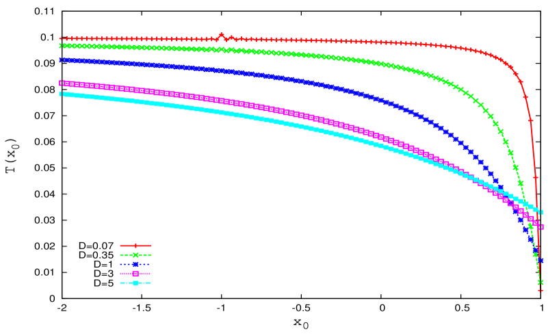
Figure 1: Nonlinear relaxation time, in arbitrary units (a. u.), as a function of the initial position $x_{0}$, for five values of the noise intensity $D$, namely: $D=0.07,0.35,1.0,3.0,5.0$. The values of the parameters are: $a=1$, $L_{1}=-10$ and $L_{2}=+10$.

The potential parameter $a$ (see Eq. (32)) is $a=1$, and the interval boundaries are $L_{1}=-10$ and $L_{2}=+10$. The integration step used to calculate $T(x_{0})$ from Eq. (40) is $\Delta y=10^{-4}$. For the initial position of the particle we focus on the range of values around the potential well, that is we consider $x_{0}\in[-2,+1]$. A monotonic decreasing behavior of the nonlinear relaxation time is shown. The NLRT decreases with initial positions moving from the left of the minimum ($x_{0}=-1$) towards the maximum ($x_{0}=+1$) of the potential and with increasing noise intensity. An overlap of the different curves appears near the maximum of the potential. This behavior could be ascribed to the role of initial positions near the maximum. For initial positions that are close to the maximum of the potential ($x_{0}=1$) the height of the barrier to cross decreases considerably and the probability of the particle to fall back into the potential well increases. For the role of the initial conditions in barrier crossing, with Gaussian noise, see Refs. [10, 11].

In Fig. 2 we report the log-log plot of the behavior of the NLRT as a function of the noise intensity $D$, for three initial positions of the particle, namely: $x_{0}=-2.0,-1.0,0$. As we can see the decreasing behavior of the NLRT with increasing noise intensity is recovered (see Ref. [21]).

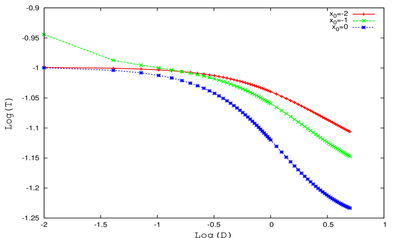
Figure 2: NLRT (a. u.) as a function of the noise intensity $D$, for three values of the initial position of the particle, namely: $x_{0}=-2.0,-1.0,0$. The parameter values are the same of Fig. 1.

4 Conclusions

In this paper we obtain the general differential equation useful to calculate the nonlinear relaxation time for a particle moving in a cubic potential and with an arbitrary Lévy index $\alpha$. For Cauchy noise ($\alpha=1$) we obtain the closed expression in quadrature of the NLRT as a function of the noise intensity, the initial position and the parameters of the potential. A monotonic behavior of the NLRT as a function of the initial position of the particle is obtained in this case. For free anomalous diffusion the NLRT decreases monotonically with the noise intensity as in the presence of the cubic potential.

References

References

- [1] Lévy P, 1937 Theory de l’addition des variables Aléatoires (Gauthier–Villars, Paris)
- [2] Gnedenko B V and Kolmogorov A N, 1954 Limit Distributions for Sums of Independent Random Variables (Addison–Wesley, Cambridge) [English translation from the Russian edition, GITTL, Moscow (1949)]
- [3] Chechkin A V, Gonchar V Yu, Klafter J and Metzler R, 2006 Adv. Chem. Phys. 133 439
- [4] Metzler R and Klafter J, 2000 Phys. Rep. 339, 1
- [5] Uchaikin V. V., 2003 Physics-Uspekhi 46, 821
- [6] Dubkov, A., Spagnolo B. and Uchaikin V. V., 2008 ”Lévy Flight Supediffusion: An Introduction”, Int. J. Bifur. Chaos 18 (9), in press
- [7] Dubkov A and Spagnolo B, 2005 Fluct. Noise Lett. 5, L267
- [8] Kramers H A, 1940 Physica 7, 284
- [9] Hänggi P, Talkner P, and Borkovec M, 1990 Rev. Mod. Phys. 62 251
- [10] Spagnolo B, Dubkov A A, Pankratov A L, Pankratova E V, Fiasconaro A and Ochab-Marcinek A, 2007 Acta Physica Polonica B 38 (5), 1925
- [11] Fiasconaro A, Spagnolo B, and Boccaletti S, 2005 Phys. Rev. E 72, 061110
- [12] Ditlevsen P D, 1999 Phys. Rev. E 60, 172
- [13] Fajans J and Schmidt A, 2004 Nucl. Instrum. & Methods A 521, 318
- [14] Gitterman M, 2000 Phys. Rev. E 62 6065
- [15] Yuste S B and Lindenberg K, 2004 Phys. Rev. E 69, 033101
- [16] Rangarajan G and Ding M, 2000 Phys. Rev. E 62, 120
- [17] Buldyrev S V, Havlin S, Kazakov A Ya, da Luz M G E, Raposo E P, Stanley H E and Viswanathan G M, 2001 Phys. Rev. E 64, 041108
- [18] Bao J-D, Wang H-Y, Jia Y and Zhuo Y-Zh, 2005 Phys. Rev. E 72, 051105
- [19] Chechkin A V, Metzler R, Gonchar V Yu, Klafter J and Tanatarov L V, 2003 J. Phys. A: Math. Gen. 36, L537
- [20] Chechkin A V, Gonchar V Yu, Klafter J and Metzler R, 2005 Europhys. Lett. 72, 348
- [21] Chechkin A V, Sliusarenko O Yu, Metzler R and Klafter J, 2007 Phys. Rev. E 75, 041101
- [22] Dybiec B, Gudowska-Nowak E and Hänggi P, 2006 Phys. Rev. E 73, 046104
- [23] Dybiec B, Gudowska-Nowak E and Hänggi P, 2007 Phys. Rev. E 75, 021109
- [24] Imkeller P and Pavlyukevich I, 2006 J. Phys. A: Math. Gen. 39, L237
- [25] Imkeller P, Pavlyukevich I, and Wetzel T, 2007, arXiv:0711.0982v1 [math.PR], 6 Nov 2007, pp 1–30.
- [26] Koren T, Chechkin A V and Klafter J, 2007 Physica A 379, 10
- [27] Sparre Andersen E, 1953 Math. Scand. 1, 263
- [28] Sparre Andersen E, 1954 Math. Scand. 2, 195
- [29] Siegert A J F, 1951 Phys. Rev. 81 617
- [30] Gardiner C W 1993 Handbook of stochastic methods for physics, chemistry and the natural sciences (Berlin) Springer.