Coherent control of localization, entanglement, and state superpositions in a double quantum dot with two electrons

Abstract

We have recently proposed a quantum control method based on the knowledge of the energy spectrum as a function of an external control parameter [Phys. Rev. Lett. 99, 036806 (2007)]. So far, our method has been applied to connect the ground state to target states that were in all cases energy eigenstates. In this paper we extend that method in order to obtain more general target states, working, for concreteness, with a system of two interacting electrons confined in semiconductor double quantum wells. Namely, we have shown that the same basic method can be employed to obtain localization, entanglement, and general superpositions of eigenstates of the system.

I Introduction

Quantum control is an area of research of great current interest with a vast potential for applications in quantum information technologies. dal ; JMO The basic problem of quantum control consists of driving externally a quantum system in order to take it from an initial state to a target final state. Quantum control ideas and methods are traditionally widely applied in magnetic resonance sli ; van-chu and quantum chemistry, sha-bru and they are advancing rapidly in the area of solid state nanostructures. bon-etal ; pet-etal ; ber ; rud

In a series of recent publications mur-wis-tam ; wis-mur-tam ; mur-wis-tam-08 we have presented a method of quantum control based on the knowledge of the energy spectrum as a function of a suitable single control parameter. This method is useful provided that the transitions between neighboring levels are well described by the Landau-Zener model.zener The latter condition has allowed us to successfully navigate the spectrum with a combination of diabatic and adiabatic changes of the control parameter. Other authors have also employed the navigation of the energy spectrum as a coherent quantum control tool, especially in the field of atomic and molecular systems controlled by lasers. vit-etal ; gue-etal ; yat-etal ; yat-etal2 ; san-etal We have applied our control method to two different physical systems with remarkable success. The first one, which we will study in this paper, is a nanostructured semiconductor system consisting of two interacting electrons confined in quasi-one-dimensional quantum dots,mur-wis-tam ; wis-mur-tam ; mur-wis-tam-08 and the second one was the LiCN molecule.licn In both systems we have been able to connect distant eigenstates through long and complex paths in the energy spectrum with very high probability.

In this paper we take the control method farther: by allowing not only diabatic and adiabatic transitions but also intermediate velocities, we can arrive at more complex final (target) states. With this generalized navigation method we are able to achieve the creation of linear superpositions of adiabatic states starting from the ground state. This opens a rich menu of possibilities, like the creation of Bell states and other types of entangled states.

The paper is organized as follows: in Section II we describe the main ingredients of our control method. In Section III we present again the two-electron nanostructure. Section IV is devoted to the results of the generalized control method. Among the results presented, we show how to apply our method to generate Bell states and coherent superpositions of energy eigenstates.

Figure 1: Schematic plot of the building block of our control method. An avoided crossing and a schematic drawing of the diabatic (fast), adiabatic (slow), and intermediate ways to cross it. (a) Long (short) arrows represent fast (slow) variations of the control parameter; (b) Medium arrows represent the intermediate velocity.

II The control method: Navigating the Hilbert space

Let us first review the basic ideas of our method in the simplest possible system, i.e. a parameter-dependent two level system. Let us assume that these two levels have an avoided crossing as shown in Fig. 1. At the avoided crossing, the two energy levels approach each other and the associated eigenstates exchange their characteristics as the external parameter sweeps through the crossing. If the avoided crossing is traversed very slowly (adiabatic path in Fig. 1(a)), the adiabatic theorem guarantees that one will stay in the initial adiabatic level, but with the paradoxical consequence that the final state will have been exchanged with the other diabatic state. On the other hand, if the avoided crossing is traversed very quickly (diabatic path in Fig. 1), the characteristics of the state are preserved. Clearly, these two limiting possibilities suggest a very simple control method. The quantitative meaning of slow and fast transitions is given by the theory of Landau-Zener transitions.zener ; mur-wis-tam-08

This basic idea has allowed us to perform complicated control tasks. Namely, we can travel through the energy spectrum using the avoided crossings as sources of efficient controllable choices between two adiabatic states. In this way we can connect distant adiabatic states provided that there exists a path going from one to the other via jumps at avoided crossing and adiabatic evolutions in the absence of crossings. Examples of the application of this method have been presented in Refs. [mur-wis-tam, ; wis-mur-tam, ].

In this paper we go one step further by using not only diabatic and adiabatic transitions but also transitions with intermediate speeds. This type of transition gives final states (on exit of the avoided crossing) which are linear combinations of the two adiabatic states (Fig. 1(b)). The combination of several crossings using intermediate velocities allows us to access a great variety of final states. Thus, in this work we generalize the control method proposed earlier and present several applications which show the power of the improved control technique.

III The double quantum dot system

Figure 2: Confining double well potential in the longitudinal direction of the coupled quantum dot structure. The external electric field is $E=0$ (solid lines) and $E=12\,\mbox{kV/cm}$ (dashed lines).

In order to explore on a concrete system the idea of using intermediate speeds to traverse avoided crossings we will study here a system of two interacting electrons inside a quasi-one-dimensional double quantum dot which was used in our previous works. The system is subject to an external, uniform electric field, whose amplitude is used as the control parameter. The confinement of the two electrons is very narrow on two dimensions, which we denote as $x$ and $y$, and the double well profile is defined along the remaining, longitudinal coordinate, $z$. The effective Hamiltonian of the two electrons reads

$$H \equiv -\frac{\hbar^{2}}{2m}\left(\frac{\partial^{2}}{\partial z_{1}^{2}}+\frac{\partial^{2}}{\partial z_{2}^{2}}\right)+V(z_{1})+V(z_{2})$$ (1)

$$+V_{C}(|z_{1}-z_{2}|)-e(z_{1}+z_{2})E(t),$$

where $m$ is the effective electron mass in the semiconductor material, $V_{C}$ is the effective Coulomb interaction between the electrons, tam-met-99 $V(z)$ is the confining potential (see Fig. 2), and $E(t)$ is the external time-dependent electric field. We choose as confining potential a double quantum well with well width of 28 nm, interwell barrier of 4 nm, and 220 meV deep (a typical depth for a GaAs-AlGaAs quantum well). We normally assume that the initial state is the ground state, which is a singlet. Since the Hamiltonian is spin independent, the total spin is conserved and the spatial wave function remains symmetric under particle exchange at all times.

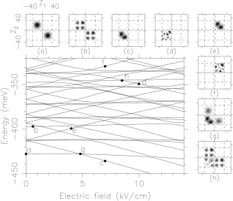
Figure 3: Main panel: The energy spectrum of the two interacting electrons confined in a quasi-one-dimensional double-well semiconductor nanostructure as a function of an external uniform electric field. The first 31 energy levels are shown. Side panels: Spatial wave functions $\phi_{i}(E,z_{1},z_{2})$ corresponding to labels (a) to (h) of the main panel. States (a) and (b) have one electron in each well, wave functions (c) and (d) are localized in the left well, and wave functions (e) and (f) have both electrons in the right well. States (a) to (f) are far from avoided crossings and therefore have well-defined localization properties. This is not the case for eigenstates (g) and (h), which are at avoided crossings.

Let us review some characteristics of the energy spectrum of the two electrons and of the eigenstates which will guide our control strategies. First we consider the spectrum as a function of the control parameter (the external electric field). This spectrum is plotted in Fig. 3 with selected eigenstates. The energies $\epsilon_{i}(E)$ and the eigenstates $\phi_{i}(E,z_{1},z_{2})$ are obtained by numerical diagonalization. For this calculation, we have used as basis set the symmetric combinations of the twelve lowest single-particle eigenfunctions. Thus, our basis set of the two-particle Hilbert space has 12*(12+1)/2=78 states. An important characteristic of this system in the lower part of its spectrum is that the states have fairly well-defined localization properties. The three possible types of localization (both electrons in the left dot, in the right dot, or electrons in different dots) are associated with the three types of slopes seen in the spectrum (positive, negative, or almost zero, respectively). In Fig. 3 we show some states to illustrate the mentioned localization characteristics. In states a and b the electrons are in different dots, in states c and d both electrons are in the left dot, and in states e and f both electrons are in the right dot. Of course, at the avoided crossing the states get mixed and these well-defined properties are lost (states (g) and (h)).

IV Results

This section is devoted to illustrate the power of the generalized control method in which the velocities to cross the avoided crossings are not restricted to produce diabatic and adiabatic transitions. In other words, we will show the possibilities opened by the ability to allow intermediate velocities. Due to the potential for applications of our method, we consider it best to illustrate its power through two important examples of coherent control.

IV.1 Localization

An application of quantum control that has been extensively explored in the recent literature is the localization of one or two electrons in a double well potential. The general idea is to start the coherent evolution in the ground state, which in the case of two electrons is delocalized due to the Pauli and Coulomb repulsions, and end up in a state in which both electrons are in the same well. In order to describe the degree of localization of the two electrons we define the probability for both electrons to be in the left well, $P_{\text{LL}}$.

$$P_{\rm{LL}}(t)=\int_{-\infty}^{0}\int_{-\infty}^{0}dz_{1}dz_{2}\,|\psi(z_{1},z_{2},t)|^{2},$$ (2)

where $\psi(z_{1},z_{2},t)$ is the evolving wave functions of the two electrons.

An easy way to localize both electrons in the left dot using our control method starting from the ground state, consists of varying the electric field adiabatically in order to pass the first avoided crossing between the first two levels located at $E=4.81\,\mbox{kV/cm}$. This process is shown in the inset of Fig. 4. (The numerical solution of the time-dependent Schrödinger equation was obtained using the usual fourth-order Runge-Kutta method with a time step of $0.05\,\mbox{fs}$.) The electric field varies linearly with time and we display the evolution of $P_{\text{LL}}$ for several velocities. We start at the ground state, and accordingly $P_{\text{LL}}\simeq 0$ at $t=0$. For a high velocity, we expect to cross diabatically the avoided crossing and the localization properties will not change considerably. This case is seen in curve (i) ($\dot{E}=4\,\mbox{(kV/cm)/ps}$.) in Fig. 4. As the velocity is decreased (curves (ii) to (v)) we approach a final state that is highly localized in the left dot. There is a maximum value of the probability $P_{\text{LL}}$ that can be obtained with this method, given by the probability $P_{\text{LL}}$ of the adiabatic ground state after the avoided crossing. The probability of the adiabatic ground state is plotted with open circles in Fig. 4. After the crossing it is a slowly rising function in the plotted range and reaches the value of 0.998 at electric field $E=9\,\mbox{kV/cm}$. We see that for the velocity of curve (v) ($\dot{E}=0.04\,\mbox{(kV/cm)/ps}$) the evolving probability $P_{\text{LL}}(t)$ follows tighlty the open circles and near $E=9\,\mbox{kV/cm}$ presents a small oscillation bound between 0.995 and 0.9975. That is, the maximum value of $0.998$ is approached within a $0.3$ percent.

Figure 4: Probability $P_{\text{LL}}$ as a function of the time-dependent electric field $E(t)$. The velocities of the electric field are: (i) 4, (ii) 1, (iii) 0.4, (iv) 0.2, and (v) 0.04 (kV/cm)/ps. With circles we represent $P_{\text{LL}}$ of the adiabatic ground state as a function of the electric field (see text for details.) Inset: closer view of the first avoided crossing involved in these processes. The arrows indicate the adiabatic path.

Figure 5: Localization with the sudden-switch method. While the electric field stays at the avoided-crossing value ($E=4.81\,\mbox{kV/cm}$) the probability $P_{L}L$ oscillates with the frequency corresponding to the energy gap (dashed lines). The method consists of increasing suddenly the electric field when $P_{L}L$ is maximal, freezing the localization on its highest value (full lines). Upper panel: Probability that both electrons are in the left dot. Lower panel: Step-wise constant electric field."

Another simple way to obtain localization in this system is what we may call the sudden-switch method, which uses step-wise constant fields.tam-met-01 We wish to compare the effectiveness of both methods to obtain localization. First, let us summarize the basic procedure of the sudden-switch method (See Fig. 5). Starting from the ground state one applies two successive steps of constant electric field. In the first step one goes from zero field to the field corresponding to the first avoided crossing, i.e. $E=4.81\,\mbox{kV/cm}$ in our case. While the new field is on, the probability $P_{\rm{LL}}$ oscillates with the frequency corresponding to the energy splitting at the avoided crossing. This oscillation occurs because the initial state is no longer eigenstate of the Hamiltonian at the avoided crossing. In fact, it is a 50%–50% linear superposition of the two adiabatic states (eigenstates) at the avoided crossing. When the probability $P_{\rm{LL}}$ reaches a maximum, that means that the current state is the other diabatic state. At this time one switches again the field to leave the avoided crossing. Far from the avoided crossing the diabatic states are very close to the eigenstates of the Hamiltonian, and therefore, are approximately stationary. Thus, the $P_{\rm{LL}}$ remains at the highest value attained during the oscillations at the avoided crossing. With this method, a localization $P_{\rm{LL}}$ of up to 93% can be achieved, as can be seen in Fig. 5. While the time scales involved in both methods are the same, in comparison, our method has three advantages: (i) a higher degree of localization can be obtained; (ii) the sudden-switch method requires a fine adjustment of the timing not needed in our case; (iii) our method is more powerful in the sense that can be used to navigate in the spectrum and connect distant states.mur-wis-tam

Let us now consider states with a different and in a sense more complex kind of localization. As mentioned earlier, we can find in the spectrum three types of localized states, which we can denote in the following way: $|RR\rangle$, $|LL\rangle$, and $|RL\rangle$, which have, respectively, both electrons in the right and left dots, and one electron in each dot. (Of course, these states cannot be considered to be product states of single-particle orbitals, because quantum correlations are generally present in all of them.cir-etal ) We usually refer to the first two types as localized states, and to the third one as delocalized. However, a linear superposition of the first two types can also be considered as localized, in the sense that one knows that both electrons would be found in the same dot if a measurement were performed. In Fig. 6 we show some control paths that may be followed in the spectrum to reach a superposition of $|RR\rangle$ and $|LL\rangle$. Linear superpositions of the form $(|RR\rangle\pm|LL\rangle)/\sqrt{2}$ are always available at the center of avoided crossings of states with RR and LL localization. In Fig. 6 (a) and (b) we show how to go from the ground state to the Bell-type states $(|RR\rangle+|LL\rangle)/\sqrt{2}$ and $(|RR\rangle-|LL\rangle)/\sqrt{2}$, respectively, using only diabatic and adiabatic transitions. We remark that these states are energy eigenstates, and thus do not evolve further if the electric field is fixed. If the restriction of using only diabatic and adiabatic transitions is relaxed we can traverse the avoided crossing of the two types of states with an intermediate speed thus obtaining a combination of the diabatic states after the crossing

$$a\,e^{-iE_{RR}t/\hbar}|RR\rangle+b\,e^{-iE_{LL}t/\hbar}|LL\rangle.$$ (3)

The values of $|a|$ and $|b|$ can be tuned by choosing the appropriate velocity. We note that the effects of using intermediate velocities was illustrated previously (Fig. 4) in the context of searching for a LL localized state.

We now show in Fig. 7 how the path (a) of Fig. 6 is obtained by varying the electric field appropriately. In Fig. 7 (a) we show the electric field and in (b) we show the probabilities as a function of time (semi-log plot). To arrive at the desired state, we must cross two avoided-crossing adiabatically, one at $E=-4.81\,\mbox{kV/cm}$ and energy $=-437\,\mbox{meV}$, and the other one at $E=3.02\,\mbox{kV/cm}$ and energy $=-402\,\mbox{meV}$. The first avoided crossing involves a RL and a RR state, and the second one, RR and LL states. The energy gap of these avoided crossings are very different, and therefore the time required to cross them adiabatically is also very different. This is way the log scale for the time axis is used in Fig. 7. We see that once the electric field is left constant the probabilities $P_{RR}$ and $P_{LL}$ oscillate between 0.465 and 0.495 while the overlap of the final state with the target one es equal to 0.98, showing that we have arrived at the desired state. The other two paths shown in Fig. 6 can be realized in a similar way, and with the same degree of success.

Figure 6: Control paths for two electrons leading to target states which are superpositions of states with RR and LL localization. The lengths of the arrows indicates the velocity of the transitions. The target states are: (a) $(|RR\rangle+|LL\rangle)/\sqrt{2}$; (b) $(|RR\rangle-|LL\rangle)/\sqrt{2}$; (c) state given in Eq. (3).

Figure 7: Numerical simulation of the path of Fig. 6(a) in order to reach the Bell-type state $(|RR\rangle+|LL\rangle)/\sqrt{2}$. The electric field used (a) and the probabilities obtained (b) are shown as functions of time in semi-log plots.

IV.2 Coherent superpositions

In the previous section we used our method to control the localization properties of the target state. Now we illustrate the flexibility of our method by obtaining coherent superpositions of several adiabatic eigenstates. For example, we may wish to obtain a linear superposition of the three types of localization having each of them the same weight. That is, we seek a state of the form

$$|\psi\rangle=\frac{1}{\sqrt{3}}\left(a|RR\rangle+b|LL\rangle+c|RL\rangle\right),$$ (4)

with $|a|=|b|=|c|=1$.

In Fig. 8 the control path to such a state is shown. In Fig. 9 we show the overlap of the evolving state with the first six adiabatic states and the electric field (the control parameter) as a function of time. To appreciate the evolution in greater detail we plot the evolving state at chosen times in Fig. 10. The initial state is the ground state (see Fig. 10, state at time $t_{1}=0$), and the final state is a superposition of the states 1, 5, and 6 at the electric field $E=3.04\,\mbox{kV/cm}$ (see Fig. 10, state at time $t_{6}=1000\,\mbox{ps}$). We start the evolution by increasing slowly the electric field (blue arrows in Fig. 8), so that the state remains at the ground state (see Fig. 10, state at time $t_{2}$), then we accelerate to cross diabatically the first avoided crossing at $E=4.81\,\mbox{kV/cm}$, and then we decrease the field (green arrows in Fig. 8) in order to cross the same avoided crossing in the opposite direction with an intermediate velocity. Here the occupation probability is split between the ground state (33.3%) and the first excited state (66.6%). This is clearly seen at time $t_{3}$ in Fig. 9. The electric field is further decreased, slowly at first and then rapidly, so that the upper branch crosses the complex avoided crossing at $E=0$ and energy of $-413\,\mbox{meV}$. Then an adiabatic increase follows. We again cross the complex avoided crossing (time $t_{4}$ in the middle of the avoided crossing and time $t_{5}$ after crossing it adiabatically). We see that the state at $t_{5}$ is a combination of a RL and a RR state. We continue slowly until the upper branch approaches the last avoided crossing at $E=3.02\,\mbox{kV/cm}$. Here the velocity is chosen at an intermediate value, so that the occupation probability divides itself equally among the two states. The end result is a superposition of the three states mentioned at the beginning. This is clearly verified in Figs. 9 and 10, state at $t_{6}=1000\,\mbox{ps}$. In this simulation, the final square overlap with the adiabatic states 1, 5, and 6 are respectively $P_{1}=0.324$, $P_{5}=0.325$ and $P_{6}=0.320$, and then the final probability to find the target state is of 96.45%.

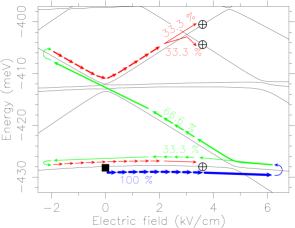
Figure 8: (Color online) Schematic diagram of the path to obtain the target which is a superposition of three adiabatic states with different localization (Eq. 4). For clarity, we use different colors when the electric field is increasing (blue and red) or decreasing (green). Our initial state, the ground state without electric field, is indicated by a filled square). The desired target state is a combination of the three adiabatic states indicated by $\oplus$.

Figure 9: Upper Panel: Electric field as a function of time used to carry out the control strategy schematically shown in Fig. 8. Lower Panel: Overlap of the evolving state with the first six adiabatic states. We can clearly see that the final state approximates well an even linear combination of the adiabatic states 1, 5, and 6 at the corresponding final electric field.

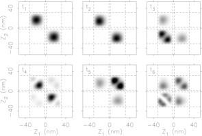
Figure 10: Evolving wave function at various times during the time evolution schematically shown in Fig. 8 and described quantitatively in Fig. 9. See text for details.

V Final Remarks

In this paper we extended a recently proposed control method for quantum systems with energy spectra, which, as function of a control parameter, are characterized by the presence of avoided crossings. While in previous publications we showed how to work with diabatic and adiabatic changes of the control parameter, that is, using the avoided crossing as a yes-no switch, here we explored the possibility of using intermediate velocities to cross the avoided crossings, thus obtaining linear combinations of diabatic states. This generalization of our previous control strategy enables us to reach more general target states, not restricted to eigenstates of the system’s Hamiltonian.

The results presented here are for a two-electron double quantum-dot structure, but are not restricted to that particular system. Since the issue of localization is an interesting one in double-well potentials, we have studied it here as an application of our method. We showed how one can obtain target states with different types of localization, like having both electrons in one given well or having both electron in either well with chosen probabilities (Bell-type states). Finally, we have shown how to obtain a coherent superposition of three states with each of the three types of localization present in this system.

References

- (1) Introduction to Quantum Control and Dynamics, by Domenico D’Alessandro (Chapman and Hall/CRC Applied Mathematics Nonlinear Science, 2007).
- (2) Special Issue on Quantum Control of Matter and Light, Journal of Modern Optics, edited by E. Paspalakis and I. Thanopulos. In press.
- (3) Principles of Magnetic Resonance, by C. P. Slichter (Springer, 1990).
- (4) L. M. K. Vandersypen and I. L. Chuang, Rev. Mod. Phys. 76, 1037 (2005).
- (5) Principles of the Quantum Control of Molecular Processes, by M. Shapiro and P. Brumer (Wiley-VCH, 2003).
- (6) N. H. Bonadeo, J. Erland, D. Gammon, D. Park, D. S. Katzer, and D. G. Steel, Science 282, 1473 (1998).
- (7) J. R. Petta, A. C. Johnson, J. M. Taylor, E. A. Laird, A. Yacoby, M. D. Lukin, C. M. Marcus, M. P. Hanson, and A. C. Gossard, Science 309, 2180 (2005).
- (8) D. M. Berns, M. S. Rudner, S. O. Valenzuela, K. K. Berggren, W. D. Oliver, L. S. Levitov, and T. P. Orlando, Nature 455, 51 (2008).
- (9) M. S. Rudner, A. V. Shytov, L. S. Levitov, D. M. Berns, W. D. Oliver, S. O. Valenzuela, and T. P. Orlando, Phys. Rev. Lett. In press. (2008).
- (10) G. E. Murgida, D. A. Wisniacki, and P. I. Tamborenea, Phys. Rev. Lett. 99, 036806 (2007).
- (11) D. A. Wisniacki, G. E. Murgida, and P. I. Tamborenea, AIP Proc. 963, 840 (2007).
- (12) G. E. Murgida, D. A. Wisniacki, and P. I. Tamborenea, J. Mod. Opt. In press. (See also arXiv:0807.4513)
- (13) C. Zener, Proc. R. Soc. London, Ser. A 137, 696 (1932).
- (14) N. V. Vitanov, T. Halfmann, B. W. Shore, and K. Bergmann, Annu. Rev. Phys. Chem. 52, 763 (2001).
- (15) S. Guerin, L. P. Yatsenko, and H. R. Jauslin, Phys. Rev. A 63, R031403 (2001).
- (16) L. P. Yatsenko, S. Guerin, and H. R. Jauslin, Phys. Rev. A 65, 043407 (2002).
- (17) L. P. Yatsenko, S. Guerin, and H. R. Jauslin, Phys. Rev. A 70, 043402 (2004).
- (18) N. Sangouard, S. Guerin, L. P. Yatsenko, and T. Halfmann, Phys. Rev. A 70, 013415 (2004).
- (19) G. E. Murgida, D. A. Wisniacki, P. I. Tamborenea, F. Borondo, F. J. Arranz, D. Farrelly, and R. M. Benito. Unpublished.
- (20) P. I. Tamborenea and H. Metiu, Phys. Rev. Lett. 83, 3912 (1999).
- (21) P. I. Tamborenea and H. Metiu, Europhys. Lett. 53, 776 (2001).
- (22) J. Schliemann, J. I. Cirac, M. Kús, M. Lewenstein, and D. Loss, Phys. Rev. A 64, 022303 (2001).