Volume dependence of Fisher’s zeros

Abstract:

We study the location of the partition function zeros in the complex $\beta$ plane (Fisher’s Zeros) for SU(2) lattice gauge theory on $L^{4}$ lattices. We discuss recent attempts to locate complex zeros for $L=4$ and 6. We compare results obtained using various polynomial approximations of the logarithm of the density of states and a straightforward MC reweighting. We conclude that the method based on a combination of discrete Chebyshev orthogonality and patching plaquette distributions at different $\beta$ provides the more reliable estimates.

1 Introduction

Locating the zeros of the partition function of lattice gauge theories in the complex $\beta$ plane and their volume dependence is important to understand the large order behavior of the weak coupling expansion [1, 2, 3, 4] at zero temperature and the nature of the finite temperature transition [5, 6]. These zeros are called Fisher’s zeros [7] and should not be confused with Lee-Yang zeros which are zeros in the complex fugacity plane or the complex $\exp(-2\beta H)$ plane [8] .

In the following, we discuss the Fisher’s zeros of a pure gauge $SU(2)$ theory with a partition function

$$Z=\prod_{l}\int dU_{l}{\rm e}^{-\beta S}\ ,$$ (1)

where S is the Wilson action

$$S=\sum_{p}(1-(1/N)ReTr(U_{p}))\ ,$$ (2)

and $\beta=2N/g^{2}$.

Our expectations is that at zero temperature, there is no singularity on the real axis of the complex $\beta$ plane and as the volume increases, the zeros stay away from the real axis. On the other hand at non-zero temperature, we expect that as the volume increases, the zeros pinch the real axis as for the 2D Ising model [7].

The zeros of the partition function can be calculated using the reweighting method [9, 5].

$$Z(\beta_{0}+\Delta\beta)=Z(\beta_{0})<\exp(-\Delta\beta S)>_{\beta_{0}}\ .$$ (3)

It is convenient to subtract $<S>_{\beta_{0}}$ from $S$ in the exponential because it removes fast oscillations without changing the complex zeros.

$Z(\beta)$ is the Laplace transform of the density of states $n(S)$:

$$Z(\beta)=\int_{0}^{S_{max}}dS\ n(S)\exp(-\beta S)$$ (4)

One can show [10] that for $SU(2)$ $S_{max}=2\mathcal{N}_{p}$ and that for lattices with an even number of sites in each direction, $n(S)=n(2\mathcal{N}_{p}-S)$, where $\mathcal{N}_{p}$ is the number of plaquettes. For a $D$ dimensional cubic lattice with periodic boundary conditions, $\mathcal{N}_{p}\equiv\ L^{D}D(D-1)/2$. When $n(S)$ is known, it is possible to calculate the partition function for any complex value of $\beta$.

In the following, we consider symmetric $4^{4}$ and $6^{4}$ lattices. For values of $\beta$ near 2, the distribution of $S$ is nearly Gaussian and the location of the peak scales with the number of sites. The departure from a Gaussian distribution is hardly visible on a histogram. However, as shown in Fig. 1, the residuals show a coherent behavior on a $4^{4}$ lattice. As the volume increases, the non-Gaussian features are scaled down and for $\beta=2.18$ it seems that the signal is lost in the statistical noise. In this figure, $N_{i}$ is the number of data points in the $i$-th bin and $P_{i}$ the corresponding probability for a Gaussian distribution with the estimated mean and variance. As in the Gaussian approximation there are no complex zeros. It is crucial to resolve the departure from this approximation. We now discuss two methods, one based on the estimation of the moments and the other on numerical calculation of the the density of states.

Figure 1: The residuals $(N_{i}-NP_{i})/(NP_{i})^{1/2}$ discussed in the text for a distribution of 500,000 values of $S$ in an histogram with 100 bins for a $SU(2)$ pure gauge theory on a $4^{4}$ lattice at $\beta=2.18$.

2 The Moments Method

In this section, we consider the following corrections [3] to the Gaussian approximation:

$$P(S)\propto\exp(-\lambda_{1}S-\lambda_{2}S^{2}-\lambda_{3}S^{3}-\lambda_{4}S^{4})$$ (5)

The four unknown parameters can be determined from the first four moments using Newton’s method. The moments are defined as

$$m_{1} = <S>/\mathcal{N}_{p}$$

$$m_{2} = <(S-<S>)^{2}>/\mathcal{N}_{p}$$

$$m_{3} = <(S-<S>)^{3}>/\mathcal{N}_{p}$$

$$m_{4} = (<(S-<S>)^{4}>-3<(S-<S>)^{2}>^{2})/\mathcal{N}_{p}$$

As $<S>$ scales like $\mathcal{N}_{p}$ and the individual terms of the $n$-th moment like $\mathcal{N}_{p}^{n}$, each subtraction implies a loss of significant digits which increases with the volume. As shown in Fig. 2 the third and fourth moments have large errors even on a $4^{4}$ lattice.

Figure 2: $m_{3}$ and $m_{4}$ for SU(2) as a function of $\beta$ on $4^{4}$ and $6^{4}$ lattices.

Once we obtain $Z(\beta)$, we can calculate the zeros of real and imaginary parts of it separately. The cross points are the Fisher’s zeros. The result for ${\beta_{0}}=2.18$ on a $4^{4}$ and $6^{4}$ lattice is shown in Fig. 3.

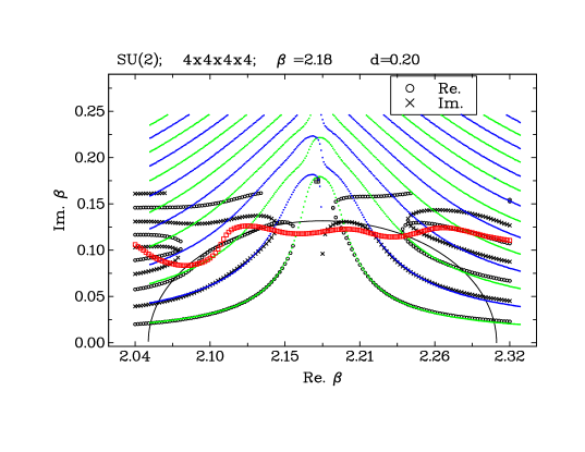
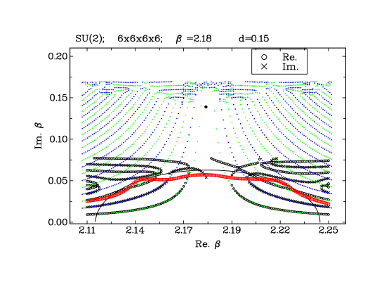
Figure 3: Zeros of the real (crosses) and imaginary (circles) using MC on a $4^{4}$ lattice, for $SU(2)$ at $\beta_{0}=2.18$. The smaller dots are the values for the real (green) and imaginary (blue) parts obtained from the 4 parameter model. The MC exclusion region boundary for $d=0.20$ (defined in [3]) is represented by boxes (red).

The errors of the moments affect $P(S)$ and the location of the zeros. A change of the fourth moment within the error bars produces changes in the zeros illustrated in Fig. 4. This change gives an idea of the errors associated with the method.

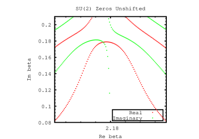
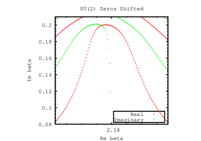
Figure 4: Changes of the zeros when the fourth moment is shifted in the positive direction until the error bar is reached for $\beta_{0}=2.18$ on a $4^{4}$ lattice.

3 Density of state Method

The probability distribution of the plaquette can be written as

$$P_{\beta}(S)=n(S)\exp(-\beta S)\ .$$ (7)

To find the $\beta$ independent density of state using Monte Carlo data, we needed to patch the data from different $\beta$ together. First the $\beta$ dependence was removed by multiplying by $e^{\beta S}$. Using only the bins with statistics higher than half the maximum, we overlay the data from each set on top of one another to make a smooth curve (we took the log of the values in the bins and adjusted the offset with a one-parameter fit). This procedure can be found with more detail in [11]. Using numerical interpolation for $f(S/\mathcal{N}_{p})\equiv ln(n(S/\mathcal{N}_{p}))/\mathcal{N}_{p}$, it is possible to calculate the zeros using numerical integration. The results are shown in Fig. 5.

As the changes were more important than expected (compared to Fig. 4), we estimated the errors by using different distributions of $S$. Three different methods are used to get the partition function, with which $<{\rm cos}(Im\beta(S-<S>))>$ is calculated and compared as a function of the imaginary part of $\beta$ at fixed real part 2.18. We estimated the error by generating multiple data. For the first, we generated 50 bootstraped sets of configurations and computed $<{\rm cos}(Im\beta(S-<S>))>$ directly by MC average. For the second, we get the partition functions via the density of states which are obtained using interpolation out of 50 patchings. For the last, we fit the 50 patchings using Chebyshev Polynomials instead of interpolation. The Chebyshev fitting seems to have much higher accuracy and stability than the other two methods and will be used for further investigations. Calculations of the zeros for $Im\beta<0.11$ with this method appear to be consistent with Fig. 3.

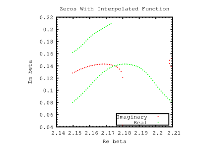
Figure 5: Same quantities as in Fig. 4 on a $4^{4}$ lattice but with an interpolated version of $f$.

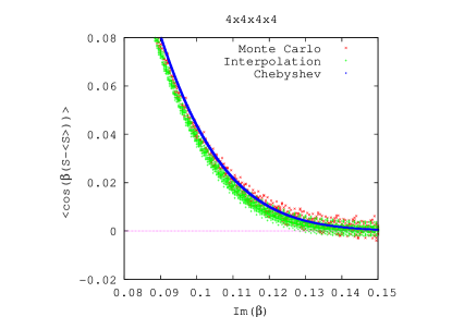
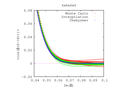
Figure 6: $<{\rm cos}(Im\beta(S-<S>))>$ as a function of the imaginary part of $\beta$ at fixed real part 2.18 with three methods: interpolation, Chebyshev fitting and bootstraped Monte Carlo, are on $4^{4}$ (left) and $6^{4}$ (right) lattices .

4 Conclusions

In conclusion, we have compared the moments methods and methods based on the density of states with the simple MC reweighting procedure to calculate the zeros of the partition function. The method where the density of states is approximated by Chebyshev polynomials seems the most reliable and will be used in future investigations.

- [1] L. Li and Y. Meurice, About a possible 3rd order phase transition at T= 0 in 4d gluodynamics, Phys. Rev., D73 036006 (2006).
- [2] Y. Meurice, The non-perturbative part of the plaquette in quenched QCD, Phys. Rev., D74 096005 (2006).
- [3] A. Denbleyker, D. Du, and Y. Meurice, and A. Velytsky, Fisher’s zeros of quasi-Gaussian densities of states, Phys. Rev. D76 116002 (2007), arXiv:0708.0438 [hep-lat].
- [4] A. Denbleyker, D. Du, Y. Meurice, and A. Velytsky, Fisher’s Zeros and Perturbative Series in Gluodynamics. PoS, LAT2007:269, 2007.
- [5] Nelson A. Alves, Bernd A. Berg, and Sergiu Sanielevici, Spectral density study of the su(3) deconfining phase transition, Nucl. Phys., B376:218–252, 1992.
- [6] W. Janke, D. A. Johnston, and R. Kenna, Phase transition strength through densities of general distributions of zeroes, Nucl. Phys., B682 618, 2004.
- [7] M. Fisher, in Lectures in Theoretical Physics Vol. VIIC. University of Colorado Press, Boulder, Colorado, 1965.
- [8] C. N. Yang and T. D. Lee, Statistical Theory of Equations of State and Phase Transitions. I. Theory of Condensation, Phys. Rev. 87 (1952) 404.
- [9] M. Falcioni, E. Marinari, M. L. Paciello, G. Parisi, and B. Taglienti, On the link between strong and weak coupling expansions for the su(2) lattice gauge theory, Nucl. Phys., B190 782, 1981.
- [10] L. Li and Y. Meurice, Lattice gluodynamics at negative g**2 , Phys. Rev. D71 016008 (2005), hep-lat/0410029.
- [11] A .Denbleyker, Daping Du, Yuzhi Li, Y. Meurice and A. Velytsky, Series expansions of the density of states in SU(2) lattice gauge theory, Phys. Rev. D78 054503 (2008), arXiv: 0807.0185 [hep-lat].