Falsifying Paradigms for Cosmic Acceleration
Abstract
Consistency relations between growth of structure and expansion history observables exist for any physical explanation of cosmic acceleration, be it a cosmological constant, scalar field quintessence, or a general component of dark energy that is smooth relative to dark matter on small scales. The high-quality supernova sample anticipated from an experiment like SNAP and CMB data expected from Planck thus make strong predictions for growth and expansion observables that additional observations can test and potentially falsify. We perform an MCMC likelihood exploration of the strength of these consistency relations based on a complete parametrization of dark energy behavior by principal components. For CDM, future SN and CMB data make percent level predictions for growth and expansion observables. For quintessence, many of the predictions are still at a level of a few percent with most of the additional freedom coming from curvature and early dark energy. While such freedom is limited for quintessence where phantom equations of state are forbidden, it is larger in the smooth dark energy class. Nevertheless, even in this general class predictions relating growth measurements at different redshifts remain robust, although predictions for the instantaneous growth rate do not. Finally, if observations falsify the whole smooth dark energy class, new paradigms for cosmic acceleration such as modified gravity or interacting dark matter and dark energy would be required.
I Introduction
A decade after the first firm evidence for the accelerated expansion of the universe Riess_1998 ; Perlmutter_1999 , the study of dark energy remains one of the most important yet difficult endeavors in theoretical cosmology (e.g. Copeland_review ; Linder_review ; FriTurHut ). The quality of data from a variety of cosmological probes has strengthened in recent years Garnavich_1998 ; Spergel_2003 ; Tonry_2003 ; Knop_2003 ; Tegmark_SDSS ; Riess_2004 ; Seljak_SDSS ; Eisenstein ; Jarvis ; Sanchez_2dF_2005 ; Astier ; Spergel_2006 ; Tegmark_LRG ; Riess_2006 ; WoodVasey_2007 ; Davetal07 ; PercivalBAO ; Guzzo ; Komatsu_2008 ; SCP_Union ; Gaztanaga , leading to multiple, independent lines of evidence for the accelerating expansion. In the near future, we can expect a battery of measurements with unprecedented precision that will provide stringent tests of any purported explanation of cosmic acceleration.
Despite the tremendous amount of raw information expected from upcoming Type Ia supernova (SN) surveys, baryon acoustic oscillations (BAO) from galaxy redshift surveys, weak lensing, and cluster counting surveys, only a handful of parameters associated with the dark energy equation of state can be constrained Linder_Huterer_howmany ; Suletal07 . This limitation arises because most observables depend on cosmological distances and growth, which are integrals over the expansion rate, which itself contains an integral over the dark energy equation of state.
Although insensitivity to fine-scale features of the equation of state is a drawback for measuring dark energy parameters, it is an advantage for testing the consistency among acceleration observables required by dark energy paradigms; since the individual probes of dark energy do not depend strongly on the rapidly oscillating evolution of the equation of state, neither do the consistency relations between these observables. For example, it is well known that under a cosmological constant explanation of acceleration or simple parametrizations of the equation of state, distance measurements predict the growth of structure in a spatially flat universe. Violation of this consistency relation would falsify the standard flat CDM model and its most basic generalizations.
The goal of this study is to extend these ideas of prediction and falsification from simple dark energy parametrizations to general classes of dark energy models with time-dependent equations of state, specifically scalar field quintessence and dark energy that is spatially smooth compared with the dark matter on small scales. We start with SN and cosmic microwave background (CMB) measurements expected in the next decade and make predictions for growth and expansion history measurements as a function of redshift within dark energy model classes parametrized by a complete basis of principal components. Where predictions are tight, observations can falsify the model class. Where predictions are loose, observations can better pin down the parameters of the class, in particular those controlling spatial curvature and dark energy that is significant at early times.
Our study complements previous work Huterer_Peiris ; Chongchitnan_Efstathiou ; Barnard_discrim on the observable predictions of classes of dark energy models, and follows a long history of studies concerning the best way to probe dark energy using cosmological observations TegEisHuKron ; EHT ; Cooray_Huterer ; Hu99 ; Huterer_Turner ; Weller_Albrecht ; Huterer_thesis ; Kujat ; Maor01 ; CorCop03 ; FriHutLinTur ; HuHai03 ; Seo03 ; Hu_Jain ; Huterer_Cooray ; Feng ; Wiley04 ; Hu_Scranton ; Upadhye ; Wang_Tegmark_2005 ; Glazebrook_Blake ; Pogosian_ISW ; Sahlen05 ; Crittenden_Pogosian ; Xia ; Hui_Greene ; Zhao ; Knox_Song_Zhan ; DETF ; Liddle_evidence ; Sahlen07 ; Zhan_Knox_06 ; Crit_Maj_Piazza ; Wang_Mukherjee_07 ; Barnard_AS ; Abrahamse_pngb ; Bozek_exp ; ZhaKnoTys08 ; Rubin_SCP . To our knowledge this is the first time that consistency between growth, distance, and other expansion observables has been studied in such a general and quantitative way. In particular, while some previous studies have considered predictions of dark energy described with a small number of parameters (e.g. Huterer_Peiris ; Barnard_discrim ; Sahlen07 ), here we consider parameters of which about are necessary to completely describe to high accuracy the predictions of current or future data. Although we compute equations of state for dark energy as an intermediate step between distance and growth, we emphasize that our goal is not to reconstruct , unlike many previous studies (e.g. reconstr ; Starobinsky ; Nakamura_Chiba ; Saini_reconstr ; Weller_Albrecht ; Gerke_Efstathiou ; Wang_Mukherjee_03 ; Sahni_review ; Li_Holz_Cooray ; Zunckel_Trotta ). Rather than addressing the quality of constraints on the equation of state, here we are more interested in using dark energy parameters only as a tool to study how to falsify basic paradigms for cosmic acceleration.
This paper is organized as follows. In § II, we describe our methods for computing predictions for observables from future cosmological data under different dark energy paradigms. These predictions can lead to falsification and subsequent generalization of each model class as shown in § III. The main tests of each class are summarized in § IV. Appendices provide additional details about the inclusion of various data in the construction of principal components and in the likelihood analysis, our methodology for computing the principal components, and tests of the completeness of our parametrization in the growth and expansion observables.
II Methodology
II.1 Dark energy principal components
We parametrize the dark energy equation of state, , with a basis of principal components (PCs) Huterer_Starkman ; Hu_PC . The PC amplitudes are weighted redshift averages of ordered by how well they are measured, and can be straightforwardly computed for a given data set. As we discuss in § II.4 and II.5, principal components based on SN distance modulus data in particular provide a nearly complete basis for other acceleration observables. We therefore treat the PC amplitudes as simply a convenient intermediate representation to capture the information in the distance modulus and translate it into predictions for other observables.
Principal components can also be defined for other redshift-dependent quantities such as the dark energy density (e.g. Hu_PC ; Dick ) which is related to by
| (1) |
where is the critical density and is the fraction of dark energy, both at the present time. Refs. Linder04 ; WangFreese discuss the advantages of using either or to describe dark energy. Our choice to use is motivated by the fact that the model classes we consider are separated by the allowed values of : for CDM and for quintessence. (Values of outside this range are possible for quintessence models in which the dark energy density becomes negative, but such models are inconsistent with current data as we discuss in § III.2.)
Specifically, we compute the PCs based on distances to Type Ia supernovae with measurement errors modeled after the proposed specifications for the SuperNova/Acceleration Probe (SNAP SNAP ) experiment. We also assume that 300 low- SNe will be available for calibrating the normalization of the high- distance-redshift relation. We supplement the SN observables with constraints on the expansion history at earlier times from the CMB acoustic peaks using the precision expected from the Planck mission. We take the CMB observables to be the matter density scaled to the present, , and the comoving angular diameter distance to last scattering, where Komatsu_2008 . Our assumptions about these fiducial SN and CMB data sets and additional priors are detailed in Appendix A. The fiducial cosmology we assume for the PC construction (and for likelihood analysis) is flat CDM with present matter fraction and Hubble constant , consistent with current data Komatsu_2008 ; SCP_Union .
The principal component functions are eigenvectors of the covariance matrix for the equation of state in redshift bins , and they form a basis in which an arbitrary function may be expressed as
| (2) |
where are the PC amplitudes, is the number of bins in redshift, and . We adopt a maximum redshift for variations in of to match the largest redshift for our fiducial supernova data, and we use a fiducial model since CDM is an excellent fit to current data. For these choices of and , Fig. 1 shows the 15 lowest-variance PCs, which form the basis we use for likelihood analysis. We comment on how the PCs depend on the choices of and the fiducial cosmology in Appendix B.
By normalizing the PCs as
| (3) |
the components approach a “continuum limit” as in which the shapes of all but the worst-determined PCs become smooth and independent of (or ). A small bin width also allows us to resolve changes in at redshifts below that of the nearest supernova in the sample, , which can evade SN constraints as discussed in Appendix B. We have chosen to use bins spaced linearly in redshift, and the exact shapes of the components depend somewhat on this choice; for example, had we chosen bins with equal widths in or , the weights of the PCs would have shifted in redshift dePutter_Linder . However, the most important property of the PCs for our purposes is that they form a complete basis for observables such as distance and growth (§ II.5), and this completeness can be achieved for a variety of different binning conventions.
Although we use a large number of redshift bins () to approach the continuum limit of the PC shapes, we generally truncate the sum in Eq. (2) to include only the modes that are measured best by the fiducial data. Predictions in § III are based on a choice of , and we explain how this number of PCs ensures completeness in various observables in § II.5.

For model classes that restrict to some range , we can place priors on the PC amplitudes analogous to those introduced in Ref. MorHu08 for reionization principal components. These priors, which we define in Appendix A, include top-hat bounds on each PC amplitude and an upper limit on the sum of squares of the amplitudes. Due to the truncation of the number of principal components required for likelihood analysis, we adopt conservative priors. A combination of PC amplitudes is only excluded if the resulting equation of state at some redshift exceeds the bounds on regardless of the amplitudes of the truncated components ( with ). Conversely, satisfying the PC priors does not guarantee that a reasonable set of truncated components can bring back within the bounds. The priors therefore include all models within a class, but do not necessarily exclude all models outside that class.
Our baseline dark energy model class is parametrized by the PC amplitudes, , and in a flat universe:
| (4) |
The Hubble constant, is a derived parameter in this representation.
In this baseline class we take the dark energy density to be constant at . The underlying assumption in this class is that by the dark energy is already much smaller than the matter density as in CDM, and enforcing constant dark energy density at assures that it becomes increasingly irrelevant at higher redshift. Note that our baseline model class includes the standard CDM model of a cosmological constant in a flat universe, corresponding to for .
II.2 Early Dark Energy and Curvature
If observations falsify the baseline model class, we can generalize it by including both dark energy that remains a substantial fraction of the energy density at , dubbed “early dark energy” Doran_Schwindt_Wett ; Doran_Robbers , and spatial curvature.
To describe early dark energy, we adopt a simple parametrization by assuming a constant equation of state, dePutter_Linder . The dark energy density at can be extrapolated from its value at as
| (5) |
This description notably accounts for, but is not limited to, scalar field models that “track” at Ratra_Peebles ; Ferreira_Joyce ; Steinhardt_tracking where the equation of state is determined by that of the dominant component, in this case matter (). We examine the limitations of this parametrization in Appendix C. Instead of , we use as the parameter for likelihood analysis since models with all have rapidly vanishing dark energy density at and are therefore degenerate with each other in all observables. We allow the early dark energy parameter to vary within the range , where the upper limit eliminates models with dark energy density that exceeds the matter density at early times. We restrict the allowed range for further in model classes where the low redshift equation of state is bounded (see Appendix A for details).
Note that components of dark matter that are smooth on small scales, for example very light neutrinos, are also described by the early dark energy parametrization. We will not distinguish between these two possibilities here as that would require measurements in a regime where either the neutrinos or the dark energy were not smooth.
To complete our most general model class, we allow for the possibility of spatial curvature, parametrized by . The full parametrization for a dark energy model class is therefore
| (6) |
The present dark energy density is derived from this parameter set. Setting and recovers the baseline model class of Eq. (4).
II.3 Markov Chain Monte Carlo
We use the Markov Chain Monte Carlo (MCMC) algorithm to estimate the joint posterior distribution of cosmological parameters and derived observables by sampling the parameter space and evaluating the likelihood of each proposed model compared with an assumed data set (e.g. see Christensen:2001gj ; Kosowsky:2002zt ; Dunetal05 ). The posterior distribution is obtained using Bayes’ Theorem,
| (7) |
where is the likelihood of the data given the model parameters and is the prior probability density. The MCMC algorithm generates random draws from the posterior distribution that are fair samples of the likelihood surface. From these samples, we can estimate many properties of the posterior distribution including the mean values, covariance, and confidence intervals of both the basic set of parameters and derived parameters and observables. Convergence of the set of random samples to a stationary distribution that approximates the joint posterior density requires a large number of independent samples. We use a minimum of four chains per model and determine when these chains have a sufficient number of samples for convergence by applying a conservative Gelman-Rubin criterion gelman/rubin of .
The full details of the simulated cosmological data and priors used for the MCMC analysis and their likelihood functions are given in Appendix A and summarized in §II.4.
We assume that all of the fiducial data are consistent with a flat CDM model with and , given that this model fits current constraints well. We therefore do not consider here the potential for SN and CMB data to test this fiducial cosmology. It is, however, possible that these future measurements will falsify flat CDM by themselves, even before considering consistency with additional observables such as growth. We have checked that most of our qualitative conclusions do not change with allowed alterations of the model underlying the SN and CMB data, and we note exceptions in Appendix C.
Given a parametrization for a model class and the fiducial data, the MCMC posterior distribution then provides observable predictions for parameters and derived acceleration observables that can be used as consistency tests to attempt to falsify the whole model class.
II.4 Acceleration observables
In this section, we define a set of redshift dependent observables that can be probed by future experiments. We focus on acceleration observables that can be simply computed from the expansion history, leaving for future study the detailed relation of these quantities to what is actually expected to be measured by specific planned experiments.
We divide the observables into two categories. In the first are observables that we assume will be measured by a SNAP-like sample of supernovae and the Planck satellite. These measurements constitute the data for MCMC likelihood analysis, from which we make predictions for the second category of observables in specific model classes.
Supernova observations constrain the distance modulus, or relative luminosity distance, between objects of different redshift in the sample. We take the SN data as a starting point since of the known methods for constraining the acceleration, it has the finest resolution in redshift and hence its principal components form the most complete set for providing testable predictions. Supernovae have an additional advantage of being sensitive to low redshifts where dark energy dominates the energy budget and where other probes like BAO and weak lensing do not have enough volume and distance, respectively, in order to strongly constrain dark energy. We take the same Planck CMB constraints on and angular diameter distance as used in the PC construction.
The SN and CMB data make predictions within a model class for the remaining observables, which include the expansion rate , the absolute distance , the growth function , and the growth rate .
The expansion rate, allowing for a general dark energy component and spatial curvature, is
| (8) |
Except when dealing with CMB observables, we generally ignore the contribution of radiation to the expansion rate since it is a negligible fraction of the density at low . The absolute distance observable we use is the comoving (angular diameter) distance
| (9) |
where the function is equal to in a flat universe (), in an open universe (), and in a closed universe (). Luminosity distances, whose ratios are measured by SNe (see Appendix A), are simply related to Eq. (9) by .
We define the growth function as , where describes growth of the matter overdensity normalized at an initial redshift during matter domination. If , then and is constant. The growth function obeys
| (10) |
where primes denote derivatives with respect to . We normalize to its value at , taking the initial conditions to be
| (11) |
where follows from a power-law solution to Eq. (10) assuming and neglecting curvature since it has little effect on the expansion rate at early times. We do not include radiation when solving Eq. (10), and we assume that the dark energy component is smooth on scales below the horizon at .
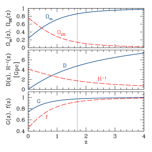
Because growth measurements can be compared either to low redshift data sets to obtain the relative growth between a redshift and the present, or to recombination through the CMB acoustic peaks to obtain , we show predictions for both in the following sections. The latter will ultimately be limited by the measurement of the optical depth to reionization from CMB polarization due to the translation between the observed acoustic peak amplitude and the intrinsic fluctuations at recombination.
The logarithmic growth rate is defined as
| (12) |
which is commonly approximated as where the growth index is for flat CDM WangSteinhardt ; Linder_gamma . Measurements of have been proposed as a way to test general relativity; we examine this idea in the context of various classes of cosmological models in § III.4.
In this paper, we remain agnostic about the techniques that best probe these observables and simply assess the precision to which they can be predicted in certain model classes. However, some caveats are useful to keep in mind. Although we make predictions as a function of redshift that can include fine-scale features, measurements will typically only constrain coarse-grained averages of the predictions over wide bands in redshift. For example, observations of the imprint of baryon acoustic oscillations (BAO) on galaxy clustering in directions transverse to the line of sight provide a standard ruler to constrain absolute distances , and BAO measurements along the line of sight can constrain the expansion rate, . However, a volume of Gpc3 is required to obtain accurate measurements of either quantity, resulting in smearing in redshift.
Likewise, weak lensing measures both the growth function and ratios of distances, but the broadness of the lensing kernel and scatter in photometric redshifts again prevents a purely local measurement. Growth rate measurements that involve the redshift space distortion of galaxy surveys and galaxy bias information from lensing suffer from broadening from both data sets. Growth and growth rate measurements from the cluster abundance or weak lensing in the nonlinear regime also involve integrals over the past history of growth and not merely the instantaneous linear growth Ma06 .
Finally, it is useful to place weak current priors on parameters related to the observables. In the broadest model classes that we consider, the SN and CMB measurements alone are not sufficiently predictive to eliminate even highly deviant models. To ensure that we only include models that are not already ruled out by observations, we include priors on the fraction of dark energy at recombination from WMAP Doran , the absolute distance from current BAO measurements from SDSS Eisenstein , and the Hubble constant from the HST Key Project HKP . The former represents the impact of the change in the growth function near recombination on the first few acoustic peaks of the CMB. We conservatively do not include the expected improvement on this measurement from Planck. The BAO distance prior serves mainly to reduce the possible deviations from a flat geometry for dynamical dark energy models with spatial curvature. The role of the Hubble constant prior in this analysis is to limit the variation in at very low redshifts as we describe in Appendix B.
In summary, the observables that we predict are the expansion rate , comoving absolute distances , the growth history relative to recombination or relative to the present, and the growth rate . The redshift evolution of these quantities for the fiducial flat CDM model is plotted in Fig. 2. Predictions from SN and CMB data are derived by constructing these observables from models in the MCMC samples described in § II.3, and we explore the implications for various dark energy model classes in § III.
II.5 Completeness
To make predictions that can reliably be used to falsify paradigms for dark energy, our parametrization must describe any effects that models within the class might have on observables. In particular, we must ensure that the set of principal components that parametrize variation in form a complete basis for representing changes in growth and expansion observables relative to the fiducial cosmology due to changes in the dark energy equation of state. In this section we summarize our criteria for completeness, and refer the reader to more detailed discussions of these issues in Appendices B and C.
When computing the PCs from the Fisher matrix for SN and CMB distances, we have a choice of whether to fix or marginalize over the parameters other than the binned . These decisions affect PC shapes due to degeneracies between and the other parameters. We choose to fix and , thereby including degeneracies with curvature and early dark energy among the well-measured PCs. We marginalize in the PC construction, thus reducing the completeness for representing sharp transitions in at as we describe in Appendix B. Since these transitions are largely indistinguishable and limited mainly by the external Hubble constant prior, completeness is not important here. We therefore choose in this instance to sacrifice completeness for efficiency in representing the well constrained redshift range.
Given the set of PCs, the next question is how many out of the full set of components we need to keep as parameters (see § II.1). Note that neglecting even the high variance PCs can have large effects on the equation of state. However, since all of the observables contain integrals over the effects of these rapidly oscillating PCs (see Fig. 1) tend to cancel out for the redshift dependent quantities of interest, especially the distance and growth observables. In general, the number of components necessary for completeness, , will be larger than the number of dark energy parameters that can be measured to some specified accuracy. We typically find that the predicted range of observables changes fractionally by less than a few percent between MCMC analyses with 10 and 15 PCs (see Appendix C). The agreement is somewhat worse for in some cases, but discrepancies occur mostly at where oscillations of about the fiducial model would be averaged out in BAO measurements over wide bins in redshift. We conclude that is sufficient for completeness, but we present results from the larger set of 15 PCs to further reduce any remaining artifacts due to incompleteness.
The completeness of the parametrization could in principle depend on the choice of fiducial model that we adopt to represent the true cosmology for future observations. We assume that the future SN and CMB data will be consistent with as is true of current measurements, and we examine an alternate choice of fiducial model in Appendix C.
Completeness may also depend on the redshift range over which the PCs are defined, . The choice of influences the definition of early dark energy as well, since we ascribe any deviations from behavior at to early dark energy parametrized by constant . We find that choosing to match the redshift coverage of the fiducial SN data nicely balances between defining the PCs where cosmological data have significant support (which argues for a lower ) and having the PCs be a complete representation for other observables (arguing for a higher ). Additionally, our parameter is not intended to be a complete description of early dark energy but rather a means of monitoring its observable signatures. We present tests of both our choice of and the early dark energy parametrization in Appendix C.
III Testing dark energy paradigms

Distance measurements from SNe and constraints from the CMB make predictions for the acceleration observables described in § II.4 that can be tested by future experiments. These predictions are made within the context of a paradigm for acceleration, e.g. a cosmological constant. Where the predictions are weak, the observables can be used to estimate parameters within the class, and where they are strong, precision measurements can potentially falsify the whole dark energy paradigm.
In the following sections, we step through the predictions for various dark energy model classes. Guided by Occam’s razor and criteria for falsifiability, we begin with the simplest model that satisfies current constraints: flat CDM. Models of this type make the firmest predictions and are therefore easiest to falsify. The next simplest and most predictive model class is CDM with one additional parameter, spatial curvature. This more general class is particularly interesting in that falsification would rule out a cosmological constant.
Since CDM corresponds to a constant dark energy equation of state , our next step in generalizing the class of models is to allow to vary with redshift. We first consider a restricted range, , corresponding to the allowed values of the equation of state in quintessence models where a canonical scalar field is responsible for cosmic acceleration at late times (e.g. CalDavSte98 ). Within the quintessence class, we study how the predictions change when early dark energy and nonzero curvature are added to the basic model.
Instead of going directly from a cosmological constant to arbitrary equations of state, one could test several intermediate models along the way such as constant or the two-parameter model Chevallier_Polarski ; Linder_wa , and many authors have used this approach in analyzing cosmological data. Here, however, we take the view that unless the dark energy falls into a well defined physical classification such as a cosmological constant or a canonical scalar field, there is no reason to define a particular functional form of as a class and not another.
For the final model class, we allow to vary over a much wider range than in the case of quintessence but retain the requirement that dark energy is smooth compared with dark matter on scales associated with the measurements of growth. For example, non-canonical kinetic terms can lead to equations of state with ArmMukSte00 . If such a field has a sound speed substantially below the speed of light, then the growth predictions presented here would only apply below its sound horizon Hu98 .
We allow an arbitrary but large range of the equation of state within of the fiducial , so . We limit the range of to enable the MCMC sampling to converge to the joint posterior distribution of the parameters more easily. This range is large enough to include extreme departures from CDM and quintessence models, particularly considering the conservative nature of our priors on PC amplitudes (see Appendix A). As with the quintessence model class, for the more general class of smooth dark energy models we also examine the effects of early dark energy and curvature on predictions for observables.
Figure 3 shows a Venn diagram representation of the model classes that we study. The CDM model class forms the innermost circle since it is a subset of all the other dark energy classes. Quintessence occupies a larger portion of the model space since the equation of state is allowed to vary within the range , and models with even more general equations of state are contained within the outer “smooth dark energy” circle. The four quadrants of this diagram separate models that are either flat or have nonzero curvature and that either do or do not have a significant fraction of early dark energy. Within each of the three model classes, an open circle marks the simplest type of model (flat with no early dark energy), and arrows lead to other models within the class with additional degrees of freedom. Since the requirement that at all times for CDM models implies that dark energy is always negligible at high redshift (see Fig. 2), the CDM class has only two types of models instead of four. See § IV for an index relating these model classes to the figures in the following sections.
The plots we present in the following sections show the range of fractional deviations in observables relative to the fiducial flat CDM model that is allowed by the assumed SN and CMB data, based on the distribution of MCMC samples. We plot these predictions for various growth and expansion observables (§ II.4) at redshifts . Any future measurements that fall outside the predicted range of values would falsify a model class.
Since it is impractical to show the whole posterior distribution at a number of redshifts for several different observables, we plot only the 68% and 95% limits of the distributions and a single example model selected from the MCMC samples. The confidence limits are defined so that the probability (i.e. number of samples) is equal at the upper and lower limits, with 68% (or 95%) of the samples between those limits. This definition corresponds to the “minimum credible interval” (MCI) of Ref. HHRW07 . A useful property of these MCI limits is that the confidence region includes the mode of the samples even when the distribution is strongly skewed.
The redshift range in our plots of observable predictions extends beyond the coverage of the assumed SN sample so that we can make predictions for observables at higher redshift. Such high redshift observations are especially important for limiting the effects of curvature and early dark energy parameters that can change observables at redshifts beyond the reach of the SN data set, although the CMB distance prior can also play this role in simpler classes of models.
There are two ways in which a model class may still be falsified even if future growth and expansion observations appear to be consistent with the SN and CMB predictions for that class. Observations that point to redshift evolution of an observable that is inconsistent with the evolution in the majority of samples would exclude the corresponding model class despite appearing to be consistent with the predictions at any single redshift. Similarly, measurements of multiple observables could falsify a model class if they are inconsistent with the predicted correlations between those observables. Since these types of inconsistencies between predictions and observations can be difficult to see in the types of plots shown here, we use the example models in each figure to help point out some of the trends in redshift and between observables.
In this study we do not address the feasibility of making the measurements required to falsify various model classes using future data sets. Instead, we focus here on determining what types of observables are the most effective at distinguishing competing theories for acceleration and what kind of precision in their measurement would be required. We leave the task of connecting our results with realistic expectations for upcoming dark energy probes for future work.
III.1 Testing CDM
The flat CDM model has only two free parameters, and , whose values are closely tied together by the CMB prior on . With this simple model, the fiducial SN and CMB data, or even the CMB data alone, make strong predictions for the other observables (see Fig. 4).
The uncertainty in the growth function at redshifts approaching recombination is zero by definition, and only increases to by (quoting CL here and throughout this section). The expansion observables at , and , are predicted with and accuracy, respectively. At low , and have equal fractional uncertainties (since ), corresponding to an accuracy of for Hu_standards . In comparison, current estimates of have uncertainties of from WMAP alone and from combined WMAP, SN, and BAO measurements Komatsu_2008 . Note that there is an extremely tight and potentially falsifiable prediction for at of in flat CDM. This prediction is driven mainly by the tight CMB distance prior which effectively reduces the remaining freedom in CDM to one parameter. In a flat universe, , so allowed variations in at high must be compensated at low by an opposing variation in to preserve .
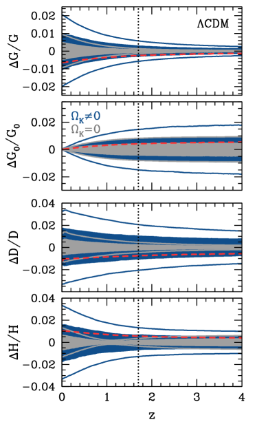
Given these strong predictions, which are in large part already available from current data, any future detection of deviations in growth, absolute distance, or the expansion rate at the percent level at any redshift would provide evidence against flat CDM. The predictions are driven mainly by the CMB prior and hence the SN data themselves can be viewed as a stringent test of flat CDM (see e.g. KLLS04 ). Conversely, testing the flat CDM predictions on other observables does not depend strongly on having the SNAP SN data set in hand.
Future observations that rule out flat CDM would indicate a need for additional complexity in the model. Although the predictions in Fig. 4 show what measurements would falsify flat CDM, they do not indicate what kind of generalizations of the model would give such alternate predictions. For example, tight predictions of at may not be so interesting if there are no reasonable models that can generate deviations from the flat CDM predictions there. Even in the context of falsifying flat CDM it is important then to look at the predictions of an extended class of models. Of the possible directions for generalizing the flat CDM model outlined in Fig. 3, we first examine the effects of including spatial curvature. We then consider the alternate option of allowing time variation of the equation of state in the following sections.
For CDM with curvature, growth and expansion predictions from the fiducial data are roughly a factor of 2 weaker than for flat CDM but remain at the percent level (see Fig. 4). The impact of the SN data is much greater when we allow curvature to vary, since the CMB constraints alone are no longer sufficient to fix the observables at low redshifts. The maximum uncertainty, at , is for and for from and . The pivot point in at also disappears, leading to the largest fractional change in the precision of predictions. In terms of measuring or constraining curvature under the CDM paradigm, the redshifts with the weakest predictions and the largest change from flat CDM offer the most fruitful epochs for measurement. Conversely, the redshifts with the strongest predictions offer the best opportunity to falsify the cosmological constant altogether. As with flat CDM, with current constraints these predictions weaken only by a factor of current .
In summary, under the assumption of CDM, with or without curvature, SN and CMB observations make firm predictions for growth and expansion observables at all redshifts. Future measurements that rule out a cosmological constant as the source of cosmic acceleration would represent a significant advance from a standpoint of fundamental physics. To proceed beyond this point and determine the best observables and redshifts to target in order to distinguish among alternate models for acceleration, we need to widen the model class again.
III.2 Testing quintessence
If measurements of growth or expansion observables exclude CDM as a viable model, the remaining dark energy model classes are ones where the dark energy equation of state at late times () is a free function of redshift (see Fig. 3). We add this freedom to the models by parametrizing with PCs as described in § II.1. We use the first PCs of at in the MCMC likelihood analysis as this number suffices for completeness in the observables to percent level precision (see § II.5 and Appendix C).
As long as the scalar field potential remains positive, the equation of state for quintessence is bounded in the interval . Negative potentials that violate this bound in the past either would not produce the required acceleration or would display easily falsifiable features. Our implementation of the canonical scalar field prior as described in Appendix A is very conservative; all quintessence models are allowed by the prior but not all models allowed by the prior can be represented as a canonical scalar field.
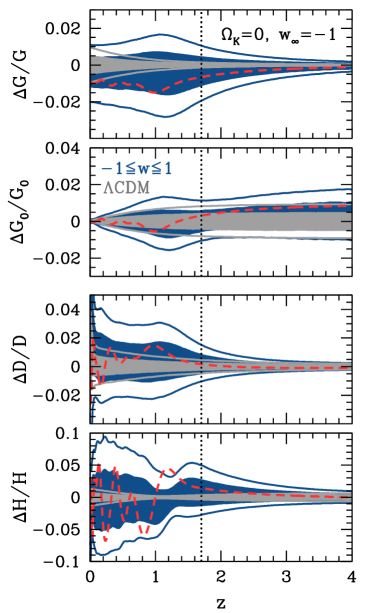
We begin in Fig. 5 with the predictions for quintessence in a flat universe with to eliminate early dark energy. Ruling out flatness in the context of CDM does not necessarily mean that curvature is required in a more general model class, so we begin with the simplest quintessence models from Fig. 3 and generalize to models with curvature and early dark energy later.
There are several notable features of quintessence predictions when compared with those in the CDM class of models. The limits on growth are no longer monotonic with redshift and in particular show that growth suppression at the level at , which would rule out CDM, is allowed in the more general quintessence context. Distances are typically predicted at a level that is about twice that of flat CDM at and comparable to CDM with curvature. The exception is at where the quintessence class allows for sharp changes in the equation of state at as described in Appendix B. The prior on the Hubble constant restricts the amplitude of such changes. Conversely, with a prior on the quintessence model class excluding these sharp transitions, precision Hubble constant measurements would play the same role as absolute distance or measurements at here and in all of the following cases.
Finally, the quintessence class allows a substantially wider range of Hubble parameter predictions . However, most of the allowed variation comes from rapid oscillations in the dark energy density, demonstrated by the example model in Fig. 5. As mentioned in § II.4, observations such as BAO that constrain are spread over a wide redshift bin, averaging out much of this oscillatory behavior. Constant shifts in the average that would be allowed by the SN measurements are still highly constrained in this model context by the CMB distance measurement. Without curvature or early dark energy, the absolute distance between and recombination is nearly fixed and thus the Planck measurement also fixes shifts in the distance scale below (see Appendix B).
The flat quintessence class of models with no early dark energy on the whole remains highly predictive and falsifiable. We next examine what kind of observations might falsify this class by requiring early dark energy or non-flat geometries.
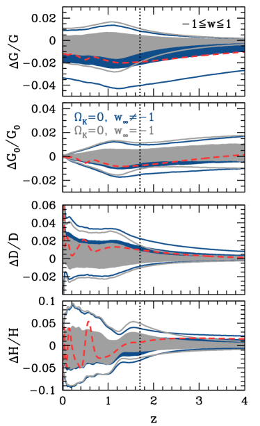
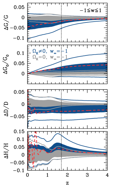
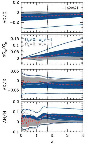
Fig. 6 shows the predictions for quintessence in a flat universe with , i.e. with early dark energy. Remarkably, the predictions for absolute distance observables remain nearly unchanged. In particular, there is no substantial increase at nor are compensating and shifts at allowed. The lack of additional freedom in the observables is mainly due to restricting the equation of state to . Early dark energy allows increased at and hence decreased distance between and recombination. To remain consistent with the CMB measurement of , these changes must be compensated by a reduction in the average and an increase in absolute distances below . Given that the fiducial model is CDM with , a roughly constant negative shift in requires dark energy to decrease with redshift, i.e. a “phantom” equation of state with . Since such values of are not allowed in the quintessence class, predictions for and remain tight even with early dark energy.
On the other hand, although growth predictions are still at the level they show an interesting feature that is a signature of early dark energy. Growth suppression at is allowed at a larger level and results in a nearly constant offset in growth at lower redshifts (see dashed curve in Fig. 6). Positive is not allowed since the amount of early dark energy can only increase from the fiducial model, which has almost no early dark energy due to the assumption of . Growth relative to , , is largely unaffected by the extra freedom allowed by early dark energy. The smoking gun of early dark energy is therefore a component to the growth function deviation that is nearly flat at .
Fig. 7 shows the predictions for quintessence in a non-flat universe with , i.e. with no early dark energy. Here the first difference is the change in the relative growth between and that is now allowed to be several percent. While both early dark energy and curvature can suppress growth relative to the early matter dominated epoch, this shift in is a unique signature of nonzero curvature. A measurement that indicates at would falsify flat quintessence models, with or without early dark energy. A measurement beyond this level (or with the opposite sign) would falsify non-flat cases as well.
The second main difference due to curvature is that high redshift negative deviations in at are now allowed at the level. A small curvature affects the distance to recombination more than it does distances at lower redshift. In an open universe, becomes larger and therefore allows dark energy the freedom to compensate by introducing a constant shift down in and up in at . The allowed amplitude of the shift is limited by our BAO prior at . Note that since the shift is constant in redshift, any single absolute distance measurement at also suffices to constrain this mode. An example of such a nearly constant shift is shown by the dashed curve in Fig. 7.
In a closed universe, the required compensation at to preserve is in the opposite direction, and as with early dark energy the quintessence prior limits this possibility. Thus one-sided deviations in , average , and growth relative to are signatures of curvature in the quintessence model class.
Fig. 8 shows the predictions for quintessence with both curvature and early dark energy. Here a much greater range of early dark energy densities is allowed since curvature in an open universe can compensate for the decreased distance to recombination due to early dark energy. The main difference is a large increase in the allowed nearly constant offset in the growth relative to recombination at which can now approach . The growth deviations are in fact limited by our early dark energy prior from WMAP (see Appendix A); without this prior the growth offset could have reached . Large suppression of the growth relative to recombination indicates both early dark energy and curvature in the quintessence context.
Note that the growth at relative to remains nearly as well predicted as in Fig. 7 with no early dark energy and hence is equally falsifiable. Likewise, predictions for do not weaken further because constant deviations in distance are limited by the BAO prior on in both cases. On the other hand, allowed models with significant early dark energy do weaken predictions for at .
Even in the most general quintessence class, there are still a few firm, percent level predictions. Neither the growth nor the distance can be appreciably larger than the CDM prediction, although both can be smaller. Lower average than in the fiducial flat CDM model is not allowed at due to the bound and at due to the CMB prior on . Suppression of growth relative to high at a level of at must remain nearly constant at . Observations that violate these predictions would falsify the entire quintessence model class.
III.3 Testing smooth dark energy
Falsification of quintessence would challenge many theories of dark energy and motivate consideration of more complicated models than single canonical scalar fields. Our generalization to the smooth dark energy class encompasses equations of state with and requires that the dark energy remain smooth compared with the matter on scales associated with growth measurements.
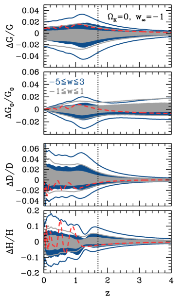
Figures 911 and 14 show the growth and expansion predictions from SN and CMB data relative to the fiducial model for the class of general smooth dark energy models. As with quintessence, we present predictions for models both with and without curvature and/or early dark energy. Remarkably, Figure 9 shows that for flat models without early dark energy the effect of dropping the quintessence bounds on weakens predictions by less than a factor of two. Thus the more general class of smooth dark energy without curvature or early dark energy is nearly as falsifiable as flat quintessence.
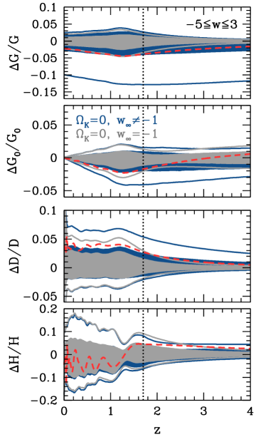
Including early dark energy in smooth dark energy models relaxes the predictions in ways qualitatively similar to the quintessence case, but with allowed deviations that are somewhat larger at 68% CL and noticeably larger at 95% CL. The additional freedom in growth and distances comes mainly from dropping the lower bound on and allowing phantom dark energy models with . This change enables a reduction of the dark energy density at from the fiducial model, which can compensate for and thereby allow a higher fraction of early dark energy while maintaining consistency with the CMB distance prior. Since dark energy is the dominant component at late times, decreasing its density typically results in lower total density at low , which increases absolute distances there. The extra early dark energy suppresses the growth at , and the reduced dark energy density at low raises growth back up toward the fiducial model slightly by . Comparing Figs. 8 and 10, we find that these models with significantly lower are the only flat smooth dark energy models that would not already be excluded if observations had falsified all quintessence models.
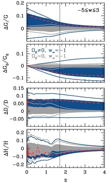
In contrast, allowing spatial curvature to vary in the smooth dark energy model class produces models with qualitatively new types of behavior not seen in the quintessence models. These new observable deviations from flat CDM provide smoking-gun signatures of curvature and an equation of state beyond quintessence.
Although some of the model classes examined so far allow growth relative to early times to be suppressed by or more compared with the fiducial flat CDM model, none of the previous cases allow growth to be enhanced by more than . However, models with weak bounds on and nonzero spatial curvature can have be as much as higher than the fiducial model at , as shown in Figure 11. Likewise, the growth relative to can be lower than in the fiducial model by or more at , whereas it was previously limited to deviations of at most a few percent in this direction. Both effects correspond to an enhancement of growth at that occurs in closed models ().
The reason why such models become viable when we abandon the prior is similar to the explanation for the differences in the early dark energy predictions of quintessence and smooth dark energy models. Closed universes have smaller distances to recombination, so without some other means to increase the distance, the models with are inconsistent with the CMB distance prior for the fiducial cosmology. Removing the quintessence bounds on allows for lower dark energy density (with ) at low , which increases the total distance to last scattering and allows closed models to match the CMB constraints. The lower dark energy density at and resulting enhancement of distances are also reflected in the predictions for and in Fig. 11. Having and lower than the fiducial value means that is higher than in the fiducial model, which also contributes to the additional growth of structure at low redshift.
Although the average at low redshift can be reduced considerably relative to flat CDM, predictions for at high redshift have a sharp lower limit. The CMB constraint on places a strong lower bound on corresponding to the expansion rate in an Einstein-de Sitter universe. Closed models can exceed this bound slightly since the curvature slows the expansion, but for allowed values of this is a small effect. This lower limit is present in all previous model classes as well but its impact is less visible.
Like the non-flat quintessence predictions of Fig. 7, the predictions for smooth dark energy models with curvature are asymmetric about the fiducial model. In fact, as Fig. 11 shows, the confidence regions are so skewed toward the closed models that the fiducial model lies on the edge of the 68% regions. This is in spite of the fact that the fiducial model has the maximum likelihood by definition, and that the definition of confidence limits we use is chosen to include the peak probability. Moreover, the allowed regions of the observables in Fig. 11 are skewed in the opposite direction of the predictions for the corresponding quintessence models in Fig. 7 and therefore appear inconsistent with those predictions, despite the fact that the quintessence class is a subset of the more general smooth dark energy class. The reason for these discrepancies is that predictions in the non-flat cases with large variations in both above and below are so weak that the shapes of priors on the PC amplitudes become important in determining the extent of the confidence regions.
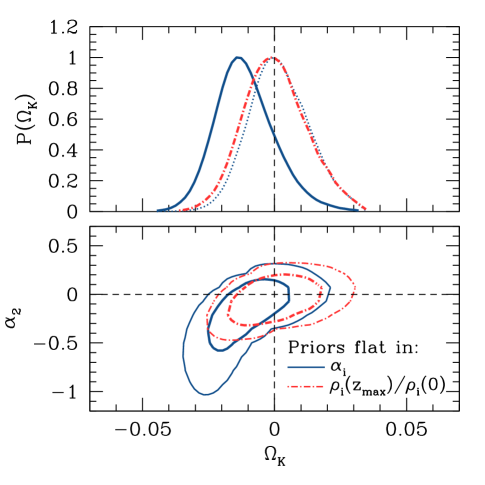
The influence of priors on the predictions is illustrated in Fig. 12, where we show distributions of for two different choices of priors. With our usual top-hat prior on , the posterior probability for is strongly skewed toward closed models. The distribution of the mean likelihood of MCMC samples, on the other hand, is peaked at the fiducial value of as expected (dotted curve in Fig. 12).
The discrepancy between posterior probability and mean likelihood can be traced to a volume effect in the parameter space (e.g. see Lewis:2002ah ). Models with more negative have a wider range of values of that fit the data well; this is demonstrated by the banana-shaped contours for and in the lower panel of Fig. 12, and other PCs show similar widening of the parameter volume at more negative . When other parameters are marginalized to obtain the 1D posterior distribution for , or for one of the growth and expansion observables at some redshift, the result is a skewed distribution.
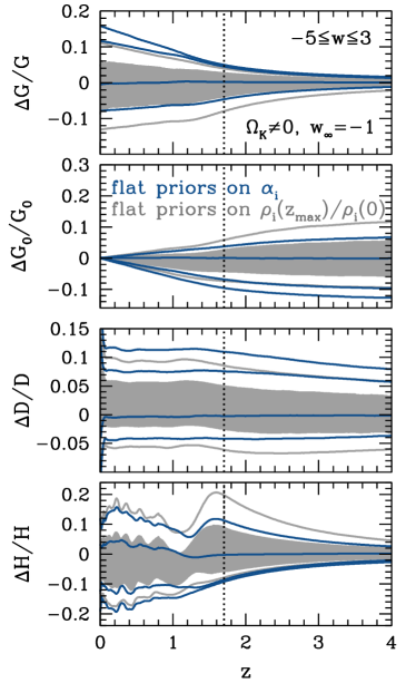
The basic reason for this volume effect is that the dark energy density depends exponentially on , which is a linear combination of the PCs, so changes in at small have less effect on observables than changes at large . To test how much the observable predictions are affected by the priors, we use alternate priors that are flat in the contribution of each principal component to the dark energy density at relative to (see Appendix A),
| (13) |
so that the total dark energy density at is . Figure 13 shows that with this new prior, the predictions become more symmetric around the fiducial model and also allow models that are acceptable under the quintessence subclass.
These shifts indicate that the predictions from cosmological data alone are so weak that the exact confidence region depends on arbitrary theoretical priors on the measure in dark energy model space. Therefore, any measurement of these observables at a level of precision comparable to the predictions is interesting in the context of smooth dark energy with curvature regardless of the sign of the deviation from flat CDM. At the same time, conclusive falsification of general smooth dark energy models with curvature would require much larger deviations where there are no models with good likelihood values.
Note that the dependence on PC priors is only significant for classes of models that allow and have nonzero curvature. For all of the previous cases – CDM, quintessence, and smooth dark energy – the confidence limits of observables shift by only when we switch from one set of PC priors to the other (except for , for which the limits change by up to a few percent at some redshifts near ). The volume effect is not a consequence of our particular parametrization of ; for example, there is a similar shift toward for non-flat dark energy models parametrized as when the priors are flat in and current .
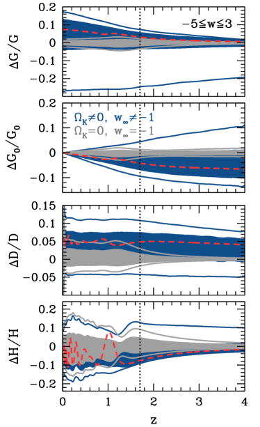
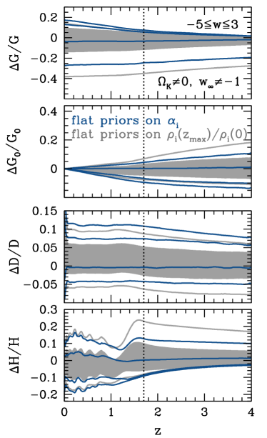
Using the priors that are flat in the PC amplitudes, the addition of early dark energy to smooth dark energy models with curvature (Fig. 14) appears to make little difference to the qualitative predictions, except in some of the 95% limits. However, much of the effect of early dark energy on these models is masked by the flat- PC prior. As Fig. 15 shows, changing the priors to be flat in affects the observable predictions in ways that are similar to the previous case without early dark energy, e.g. making many of the distributions of allowed models more symmetric around the fiducial model. With this alternate prior we see that the additional freedom in early dark energy combined with nonzero curvature enables models with significant growth suppression relative to high and increased to fit the assumed data sets, as it does in the corresponding quintessence predictions of Fig. 8.
The sensitivity to the priors and the weakness of the predictions in general means that despite the great potential of future observations for measuring spatial curvature and early dark energy in models with general equation of state variation at low redshift, statements about falsification of the entire smooth dark energy model class must be made with care.
III.4 Beyond Smooth Dark Energy
One lesson from the analysis in the previous section is that the combination of general variation in the dark energy equation of state with early dark energy and nonzero spatial curvature allow a wide variety of cosmological models to fit future SN and CMB data. Falsification of the most general smooth dark energy model class therefore appears to be quite difficult, especially given the dependence of the growth and expansion observable predictions on priors that must be set arbitrarily in the absence of an underlying theory for dark energy. However, even these very general models make some firm predictions about the relations between observables that could potentially be falsified by future measurements.
One example of a robust prediction for the observables is the following: given the flat CDM model that matches the SN and CMB data and assuming that the dark energy always contributes positively to energy density, at can be no more than lower than in CDM. This limit was noted in § III.3) in the context of non-flat smooth dark energy models with , and it still holds when we include early dark energy.
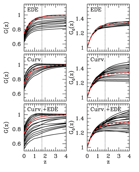
More interestingly, the predicted redshift evolution of expansion and growth observables still exhibits certain regularities. Notice in Fig. 10 that before we introduce curvature, the growth history, absolute distances, and expansion rate are predicted at the few percent level by SN and CMB data. Freedom in the spatial curvature greatly reduces the precision of these predictions. However, the curvature is set by a single parameter with well defined effects on each of the observables. By taking advantage of our knowledge of the impact of curvature, we can effectively regain much of the predictive power that exists for flat models.
As an example, consider the growth function. In the most general model class, the majority of the freedom in growth comes from curvature and early dark energy. We can distinguish between the two by noting that the deviations in growth from the fiducial flat CDM model have different redshift dependence, as illustrated by the sample growth histories allowed by either curvature or early dark energy plotted in Fig. 16. The main effect of early dark energy is to suppress growth by a constant factor at early times, so growth functions in a flat universe with varying amounts of early dark energy have similar shapes but different amplitudes at low . On the other hand, curvature tends to have a more gradual effect on growth continuing to , and also allows more enhanced growth relative to the fiducial model than early dark energy.

An observed growth history that cannot be described by some combination of the effects of curvature and early dark energy would present a major challenge to the dark energy paradigm. For example, growth at relative to today () that is higher than expected in flat CDM would be difficult to explain with dark energy for allowed values of the spatial curvature.
Moreover, deviations in are nearly a one parameter family that is ordered by curvature . The top panel of Fig. 17 shows the correlation between and a linear combination of and in smooth dark energy models. The curvature mainly depends on , but the degeneracy in between at and early dark energy introduces a small correction since such changes in the expansion rate affect the growth rate at low and therefore change . The term can correct for this degeneracy since the amplitude of is sensitive to the amount of early dark energy.
By comparing the combination of and correlated with curvature at multiple redshifts, one can test the general class of smooth dark energy models with early dark energy and curvature. For example, the lower panel of Fig. 17 shows these combinations of growth observables at and at ; observations that give different values for the linear combinations of and at these two redshifts would falsify this most general model class.
This regularity in the growth relative to today can be viewed as a generalization of tests involving the linear growth rate . In particular, the relationship with has been proposed as a potential test of all smooth dark energy models Linder_gamma ; Hut_Lind_MMG ; LinCah07 ; PolGan08 ; Acqetal08 . In Figs. 1820, we plot the predictions from the forecasted SNAP supernovae and Planck CMB data for the growth rate and growth index for selected model classes from the previous sections, allowing a redshift dependent growth index
| (14) |
Note that the growth index is somewhat different from our other observables since measurement of requires not only the growth rate but also some method for determining the fractional matter density at the same redshift. A measurement of combined with the CMB constraint on could provide an estimate of the latter quantity, since .
In the context of CDM, Figure 18 shows that both and are precisely predicted by future SN and CMB data as expected given the tight constraints on other observables within this model class. The growth index is nearly constant, with a small slope at low redshifts when the cosmological constant dominates, and deviations of by for models with nonzero curvature.
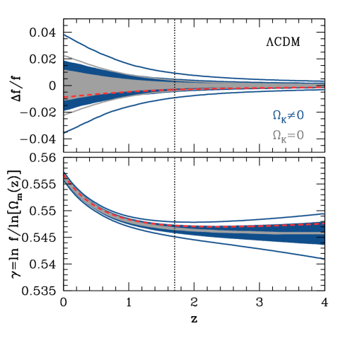
In the context of quintessence, both predictions weaken substantially as shown in Fig. 19. The growth rate is not as well predicted as the difference in growth between and used in Fig. 17. Like , it effectively has only one integral over the time-varying equation of state instead of two as for distances and the integrated growth history. It is therefore equally sensitive to features in .
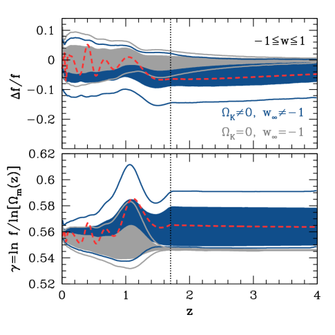
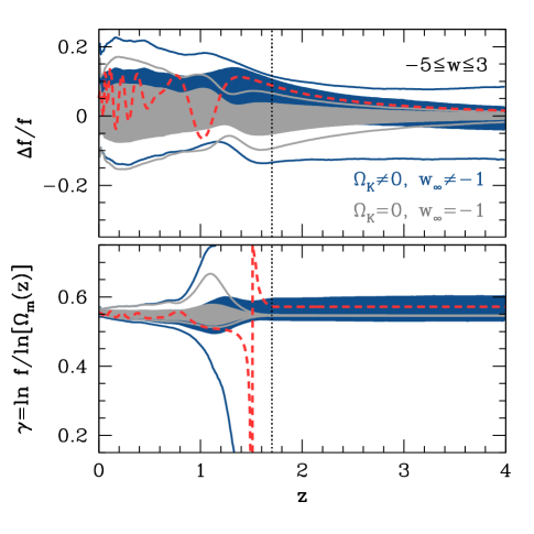
In fact, the redshift dependence of the predictions for in Fig. 19 closely mimic those for in Fig. 8, but with opposite sign. Since is tied to via the CMB prior on , the similarity between deviations in and in suggests a strong connection between and , consistent with a constant value of . However, the predicted values of shown in the lower panel of Fig. 19 cover a much wider range for quintessence than for CDM, with significant variation of with redshift in some models. For flat models without early dark energy, the extra freedom in only appears at , but including curvature and early dark energy allows deviations in above the fiducial value at , only slightly less than the uncertainty in or at these redshifts. These nearly constant deviations in at high are well approximated by the expected dependence on early dark energy given by Ref. LinCah07 , modified for nonzero curvature,
| (15) |
where . For and we recover the usual growth index from this formula, .
One of the more interesting features of the predictions for in the quintessence class is the widening in the uncertainty at . As Eq. (15) shows, deviation from changes the value of at high redshift. Likewise, low-redshift variation in can perturb the growth index from its usual value of . At , SN distance constraints ensure that while may oscillate rapidly with redshift, it never deviates far from on average. However, as approaches the constraints from SNe weaken, allowing to vary significantly from over longer periods of time; this variation enables to deviate from the CDM prediction. Furthermore, at where is typically near unity, is close to zero and therefore the value of derived from Eq. (14) is more sensitive to small changes in the relation between and . For example, the model plotted in Figs. 8 and 19 has significant changes in and between and relative to the fiducial flat CDM cosmology, leading to a bump in for this model at .
Generalizing to smooth dark energy models with reveals another potential problem with using to test smooth dark energy. Recall from the previous section that a closed universe is allowed for models in this class, and is favored if priors are flat in the PC amplitudes. In closed models where is sufficiently negative, can cross unity with at high and at low , and the same is true of . Since these two functions do not cross at exactly the same redshift due to the slight lag between density and growth, the growth index of Eq. (14) has a singularity when . The dashed curve in Fig. 20 is one example of such a model. As a result, the predictions for , particularly in the tails of the distribution, blow up at where these singularities occur. This effect is an artifact of the parametrization since can take any value when and , but it makes it difficult to interpret limits on beyond for the most general class of smooth dark energy models.
Although constant remains a good approximation for many dark energy models, large variations in the dark energy density or spatial curvature with can weaken the link between and (or ). An observed deviation from the expected value and near constancy of would certainly falsify CDM and some simple dark energy models, but using the growth index as a test of smooth dark energy in general may require refinement of the standard parametrization of Eq. (14) to account for significant variation and crossing of . Alternatively, one can adopt the more general approach of examining the integrated growth function at various redshifts as discussed above.
There are also other, more fundamental but more qualitative means of testing smooth dark energy. By definition, on scales where the dark energy remains smooth there is no particular scale for growth in the linear regime. Models of acceleration that involve coupling of dark energy to dark matter or modifications of gravity that introduce new scales in addition to the Hubble scale generically imply scale dependent linear growth (e.g. WhiKoc01 ). Such models can also feature differences in dynamical and lensing mass measurements. Generically, modified gravity models that satisfy local constraints on gravity also break the relationship between the linear and nonlinear growth of structure again by the introduction of a new scale to the problem Vai72 ; HuSaw07 ; OyaLimHu08 .
Another way in which the standard cosmological paradigm might be falsified is through observed violations of the relation between luminosity distances and comoving angular diameter distances. Examples of mechanisms for violating this relation include photon-axion mixing, photon decay, and nonzero torsion in the gravity theory (e.g. Bassett_Kunz_03 ; Uzan04 ; SonHu05 ). Therefore, the “duality relation” between the two distances is an interesting test of exotic new physics possibly related to acceleration. There also exists a more general (but related) consistency relation between the comoving distance and the Hubble parameter that holds in any homogeneous and isotropic FRW model Clarkson_Bassett and can be tested using accurate cosmological observations of the two functions at any redshift. Our standard assumptions could also be falsified through observed violations of homogeneity or isotropy signaling a breakdown in the validity of the FRW metric, or by observing time variation in fundamental constants.
We have shown that dark energy degrees of freedom and spatial curvature permit the basic distance, expansion, and growth observables to vary greatly. Nevertheless, there are still many ways in which the dark energy paradigm for acceleration could be falsified.
IV Conclusions
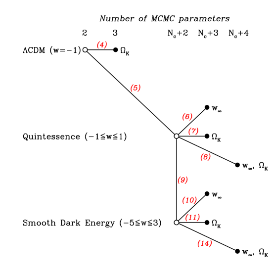
Using a combination of quantitative tools including principal components of the dark energy equation of state and MCMC analysis with simulated future data, we demonstrate that combined constraints on dark energy from the measurement of distances, growth, and the expansion rate provide many ways to test not only specific dark energy models, but also general classes of models. In particular, a high-quality supernova sample such as that anticipated from SNAP and the CMB data expected from Planck make strong predictions for other observables in the context of a wide variety of models. Follow-up observations of the predicted observables offer the exciting possibility of falsifying model classes and demonstrating the need for a new paradigm for acceleration.
Figure 21 summarizes the basic dark energy model classes and their generalizations, arranged by the allowed values of and the total number of MCMC parameters [Eq. (6)]. In general, observations that falsify classes toward the upper left corner of this “tree” of model classes require adding more freedom to the models by moving down and/or to the right in the tree. This diagram serves as an index to the figures in § III; each line between a pair of model classes is labeled by the number of the figure in which a comparison of observable predictions for those two classes may be found.
In the context of the current standard model, flat CDM, predictions for acceleration observables come mainly from the CMB. The SNAP SN data themselves provide one stringent test of flat CDM predictions from Planck. Other types of observations are also well suited for testing flat CDM. In particular, constraints from future SN and CMB data have a narrow pivot point in the expansion rate where is predicted to (at 68% CL), making such a measurement an especially interesting target for future BAO experiments and other probes of . Likewise, growth observables are predicted to better than at all redshifts.
Even if we drop the assumption of flatness, CDM remains highly predictive. The pivot point in predictions disappears when nonzero spatial curvature is allowed, but the CDM model class can still be falsified with deviations in any of the acceleration observables at any redshift.
Remarkably, allowing general time variation of the dark energy equation of state within the class of quintessence models () does not significantly weaken predictions if we assume flatness. For these models, SN and CMB data predict growth and absolute distance to precision.
Including the possibility of early dark energy, e.g. a scalar field that tracks the matter density at high redshift, does not weaken these predictions substantially as long as the SN and CMB observations remain consistent with a cosmological constant as current data suggest. An increased fraction of early dark energy reduces the distance to recombination, , and must be compensated by either allowing nonzero curvature or reducing the dark energy density at late times. The latter option requires which is forbidden for quintessence models with positive potentials, so a large fraction of early dark energy is not allowed for quintessence in a flat universe.
The same barrier for quintessence leads to predictions of one-sided deviations from flat CDM observables when spatial curvature is allowed to vary. Closed universes reduce , so matching CMB constraints requires the ability to lower the dark energy density with . Therefore, quintessence predictions from SN and CMB data consistent with favor open universes. Curvature in open universes causes additional growth suppression, particularly at .
Open quintessence models can also have significant early dark energy that suppresses growth by a constant factor at low redshift. Even with the additional freedom in curvature and early dark energy, SN and CMB data still provide general predictions for quintessence. For example, neither the growth relative to recombination nor absolute distances at low redshift can be significantly larger than in flat CDM. Growth relative to the present out to cannot differ from its standard behavior by more than .
Allowing the low-redshift dark energy equation of state to vary beyond the range of quintessence enables new types of models since the absence of the bound permits deviations in dark energy density both above and below the constant density of flat CDM. These general smooth dark energy models are therefore able to have significant early dark energy in a flat universe, and closed universes consistent with the SN and CMB data are also possible. As a result, smooth dark energy models can have both larger and smaller growth and absolute distances relative to flat CDM, unlike the one-sided predictions of quintessence.
Even the most general model class including large dark energy variations at low redshift, early dark energy, and nonzero curvature makes some generic predictions given future SN and CMB data. Growth at normalized to its present value can be no more than larger and the expansion rate at no more than smaller than their values in a flat CDM cosmology. The growth index as it is typically defined is tightly constrained by SN and CMB data in CDM, but not for more general dark energy models since both time variation of the dark energy equation of state and the possibility of crossing in closed universes weaken the relation between growth rate and matter fraction. Fortunately, growth measurements at different redshifts still give tight predictions since the growth evolution at low redshift depends mainly on curvature. Additional tests outside the scope of this work, such as searching for scale dependence of linear growth, could also falsify all smooth dark energy models. Falsification of the most general smooth dark energy predictions would require new paradigms for cosmic acceleration and possibly even gravity itself.
Acknowledgments: We thank Eric Linder, Hiranya Peiris, and Amol Upadhye for useful conversations. MM and WH were supported by the David and Lucile Packard Foundation and the KICP under NSF PHY-0114422. MM was additionally supported by an NSF Graduate Research Fellowship. WH was additionally supported by DOE contract DE-FG02-90ER-40560. DH was supported by the DOE OJI grant under contract DE-FG02-95ER40899, and NSF under contract AST-0807564.
Appendix A Fisher Matrices and Likelihood Functions
In this Appendix, we describe the (future) cosmological data and priors that we assume for this study. We give expressions for the Fisher matrices for these data, which we use to compute the principal components of the dark energy equation of state, and for the likelihood functions that we use in MCMC analysis.
The Fisher matrix for supernovae is TegEisHuKron
| (16) |
where is the average magnitude of the SNe in the redshift bin denoted by , is the error in the average magnitude, and is a constant related to the unknown absolute magnitude of the SNe.
For the fiducial supernova data, we take the expected redshift distribution for SNAP KLMM_SNAP plus a low- sample of 300 SNe at . The SNAP magnitude errors include both statistical and systematic components:
| (17) |
where is the number of SNe in each bin of width ( except for the statistical uncertainties in the low- SN bin, for which ), and is the width of the sub-bins used to smooth the distribution of SNe in redshift. We use 500 sub-bins up to . The second term on the right hand side of Eq. (17) models a systematic floor that increases linearly with up to a maximum at of mag per bin LinHut_highz .
For the Planck CMB constraint, we start with the covariance matrix for the parameters
| (18) |
Here is the comoving angular diameter distance to recombination. We ignore additional CMB information about dark energy from the ISW effect except in the current prior on early dark energy described below. The elements of the covariance matrix are and and . Rotating to the space of MCMC parameters, e.g. [Eq. (6)] gives , where . As we shall see, for the likelihood evaluation it is more convenient to project the MCMC parameters onto the original basis of Eq. (18). For a similar treatment of CMB priors on dark energy models, see Refs. Hu_standards ; Dick .
Priors on additional parameters can be included by adding the assumed inverse covariance to the appropriate entry of the Fisher matrix. The Fisher matrix for the full set of parameters is
| (19) |
The priors and the parameters in the Fisher matrix depend on the particular application and differ between the PC construction and the the likelihood analysis. The procedure for computing PCs from the Fisher matrices and the assumed priors are described in Appendix B.
For the MCMC analysis described in § II.3 we assume a Gaussian likelihood, , described by
| (20) |
which includes contributions from the SNAP SN data, Planck CMB data, and our external priors.
We model the SN term as
where refers to the difference between a model derived from MCMC parameters and the fiducial value. The variance is modeled as in Eq. (17).
The term in comes from the marginalization over . Because of this marginalization, the SN data are insensitive to redshift-independent shifts in the magnitudes caused by changes in combinations of other cosmological parameters, e.g. and the PC amplitudes for . This shift in magnitudes corresponds to multiplying the distances by a constant factor: .
The CMB contribution to is
| (22) |
where is the same as in Eq. (18) and is the difference in and from the fiducial model with derived from the MCMC parameters.
When computing we set the SN magnitudes, , and to have the exact values predicted for the fiducial cosmology without any scatter in the simulated measurements. The resulting constraints from the data are therefore expected to be centered on the fiducial parameter values rather than shifted away from them by . We do this because we are mainly interested in the width of predictions for observables and not their central values for a particular realization of the measurement errors.
In the MCMC likelihood analysis we employ three external priors based on current data to limit our study to reasonable cosmologies, and one internal theoretical prior:
| (23) |
where the terms on the right hand side respectively refer to an HST Key Project prior on the Hubble constant of width HKP , a BAO prior on the angular diameter distance to with , roughly corresponding to the constraint from the SDSS LRG sample Eisenstein , and a WMAP prior on the fraction of early dark energy with , based on the constraints on early dark energy models in Ref. Doran .
In addition to constraints from current data, the last term in Eq. (23) includes theoretical limits on the dark energy equation of state, . These limits are typically implemented as an infinite barrier in corresponding to some range allowed by the model class, i.e. a top hat prior on the MCMC parameters. To compute these priors, we start with the projection of onto PC amplitudes,
| (24) |
where unless otherwise specified. By finding the values of within the allowed range that maximize or minimize , we obtain limits on the amplitude of each PC, , where
| (25) |
The width of this prior, , depends on the width of the allowed range of but not the value of .
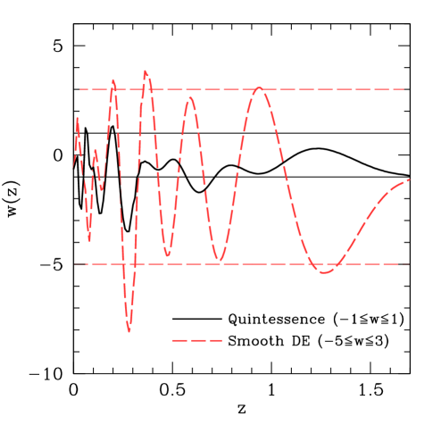
We find a second prior on using the fact that restricting the range of places an upper limit on . From Eqs. (2) and (3),
| (26) |
The bounds on impose an upper limit on this sum,
| (27) | |||||
Combining Eqs. (26) and (27) we find that the PC amplitudes must lie within a sphere in the parameter space:
| (28) |
where is the number of components in the truncated set of PCs used for likelihood analysis (see § II.1). For a given allowed range of , the constraint on PC amplitudes from this inequality is strongest when the fiducial model lies in the center of that range, , but in general the limits in Eq. (25) are the stronger of the two PC priors.
Figure 22 shows examples of parametrized by 15 PCs that satisfy the bounds in Eqs. (25) and (28) corresponding to the quintessence model class, with and , and the smooth dark energy class, with and . In each case, the sum of the 15 components is allowed to violate the bounds on at some redshifts. For some models, the addition of higher-variance PCs can correct for these deviations from the allowed range so that everywhere. However, this is not necessarily true for all models that satisfy the PC priors; the most important property of these priors is that they retain any model that does obey the limits on while excluding a large number of unacceptable models. For more details on the derivation of these priors, see Ref. MorHu08 where similar bounds are used in the context of reionization models to constrain the ionized fraction of hydrogen to the range .
When switching to alternate priors to test volume effects related to curvature as described in § III.3, we transform the PC priors either by adding an additional term to the likelihood in the MCMC analysis or by modifying the weights of samples in the chain as a post-processing step. In either case we convert the usual top-hat PC priors to ones that are flat in the density of each PC at relative to [Eq. 13] by multiplying or the sample weight by , where
| (29) |
In addition to priors on the low- equation of state, we place a top-hat prior on the early dark energy at corresponding to . Since the early dark energy MCMC parameter is actually , in practice the prior we use for MCMC is for quintessence and for smooth dark energy.
Appendix B Principal component methodology
To compute the principal components of from the Fisher matrices of Appendix A (with specified below), we first take the submatrix of corresponding to the redshift binned dark energy equation of state, . We then invert the matrix to get , which is the original Fisher matrix marginalized over everything except . Finally, we compute the eigenvectors of , which are the PC functions and normalized as in Eq. (3), and the eigenvalues, which are the inverse variances of the PC amplitudes.
We evaluate at the same fiducial model as for the MCMC likelihood, i.e. flat CDM with and . This model is consistent with current data, which should minimize the number of principal components needed to accurately parametrize viable dark energy models. The exact choice of fiducial cosmology is unimportant as principal component shapes do not vary greatly with changes in the fiducial model that are consistent with current data.
Our default binning scheme is bins between and . These bins are fine enough to obtain reasonably continuous PC shapes and to allow varying at , which has important consequences as we describe later.
We choose to match the assumed maximum redshift of the SN sample. A smaller choice of would not significantly change the PC shapes at lower but would result in a less complete set of PCs due to neglecting some of the SN data. Increasing would require additional support from SNe or other data at for the PCs to have any weight at higher redshift; the CMB distance constraint helps somewhat but is still only a single data point for constraining the additional . Furthermore, if the expansion history at low is near the fiducial flat CDM model then the lack of weight in the PCs at high is mainly a consequence of dark energy becoming less significant as redshift increases Huterer_Starkman .
Unlike the MCMC likelihood analysis, we do not include external priors from current data or priors on PC amplitudes in the term. However, we do use priors that correspond to fixing certain parameters besides , i.e. , , and . In the rest of this section we explain our choices of which of the other parameters are fixed and which are marginalized over. Note that we do not consider here because it is nearly fixed automatically due to the constraint in .
The question of fixing or marginalizing parameters is essentially a question of whether or not we wish to include degeneracies between those parameters and in the low-variance PCs that we retain for MCMC analysis. Marginalizing these other parameters eliminates from the low-variance PCs the modes in that have a degenerate effect in the SN distances and CMB data but are not necessarily degenerate in other acceleration observables. Since this marginalization generally results in an incomplete PC basis, the better choice is typically to fix the non- parameters with so that the modes of degenerate with them are assumed to be well measured and therefore are included in the low-variance PCs. Fixing these additional parameters ensures that the PCs we use are as complete as possible in the acceleration observables, and so we fix and when computing the PCs. However, is an exception to this rule where having a fully complete basis for is not desirable.
There are two types of degeneracy that can in principle exist between and in the assumed SN and CMB data. First, the dark energy can mimic some fraction of the matter density (leaving unchanged) by approaching at high (e.g. Kunz07 ). In the context of a spatially flat geometry with no early dark energy, this degeneracy is eliminated by the CMB constraints on and . The impact of these constraints weakens if we allow for the freedom to adjust either curvature or early dark energy. By constructing PCs with curvature and early dark energy fixed, we assume that the matter-mimicking mode of can be measured by the SN distances and CMB constraints. This assumption ensures that the PCs are complete with respect to this mode, regardless of whether we marginalize or fix in the PC construction. This type of degeneracy between and is therefore properly included in the MCMC predictions for model classes with curvature and early dark energy.
A second type of degeneracy is introduced by the minimum redshift for which SNe can be measured in the Hubble flow. The ability to determine from SN observations depends on how well we can anchor the relative distances to . As noted in Appendix A, marginalization over the nuisance parameter causes the SN observations to be insensitive to constant shifts in relative distances of the form
| (30) | |||||
We are not free to change at all redshifts since at low independent of the cosmology. However, it is possible (if unlikely) that a large variation in near changes the SN distances by a nearly constant factor at all redshifts except at , where is the minimum SN redshift. When including the CMB data this effect creates a degeneracy between and since the shift in Eq. (30) requires changes in and to satisfy CMB constraints on and .
If we fix when computing the PCs, then we assume that the behavior of at is well constrained and therefore large variations in the equation of state at low redshift are included in the low-variance PCs. Instead, we choose to reduce the impact of this degenerate mode of by marginalizing in the PC construction. Our basis for is therefore incomplete with respect to this mode, but there are several reasons for neglecting large variations in at . One benefit of this approach is that by reducing the degeneracy between and the PC amplitudes we improve convergence of MCMC samples; in the presence of the full degeneracy, it is difficult to obtain well-converged chains even for the simplest class of models with PC-parametrized . Furthermore, apart from the Hubble constant itself and the interpretation of SN data as measuring as opposed to , acceleration observables are not significantly affected by this degeneracy. Finally, despite marginalizing when computing PCs we still retain enough of this degeneracy that predictions for the behavior of and is appropriately uncertain and limited by our prior on , as shown in Fig. 5, for example.
Improving measurements of beyond the current level would further limit the possibility of these ultra-low redshift changes in . Conversely, in the absence of such variation in , precision measurements play the same role as low redshift and measurements in all cases considered in the main paper.
In summary, when constructing the PCs we take priors that fix and but marginalize . We do not employ the additional current priors from BAO distance to , HST Key Project measurement of , or WMAP limits on early dark energy that are added to the likelihood analysis.
Appendix C Completeness Tests
When making predictions for general classes of models, we need to make sure that the parametrization we use has sufficient freedom to explore all types of effects that models can have on the acceleration observables. In this appendix we present several tests of the completeness of our parametrization. We begin by justifying the number of principal components of used in the MCMC likelihood analysis. We then examine the sensitivity of our results to the choices of fiducial model and maximum redshift for principal components. Finally, we discuss the limitations of our early dark energy parametrization.
The PCs form a complete basis for ordered by how well they can be measured by the fiducial SN and CMB data. This ordering allows us to truncate the set of PCs to some small number that have the greatest impact on the fiducial data. Retaining a limited number of PCs is a practical necessity to make parameter estimation feasible, but we must make sure that the higher-variance PCs that we ignore do not make significant contributions to the expansion or growth observables predicted in the main paper.
It is important to emphasize that we do not expect or demand completeness in unobservable quantities like itself; the high-variance PCs that we neglect can have large effects on the equation of state, but since all of the observables contain integrals over the effects of these rapidly oscillating PCs (see Fig. 1) tend to cancel out for the redshift-dependent quantities of interest. This is especially true for distances and integrated growth, each of which involves essentially two integrals of over redshift. Completeness is more difficult to attain for observables with a single redshift integral such as the expansion rate and growth rate, but the practical requirement of a large volume for such observations makes any rapid evolution with redshift unobservable in practice.
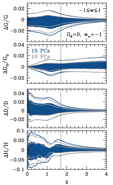
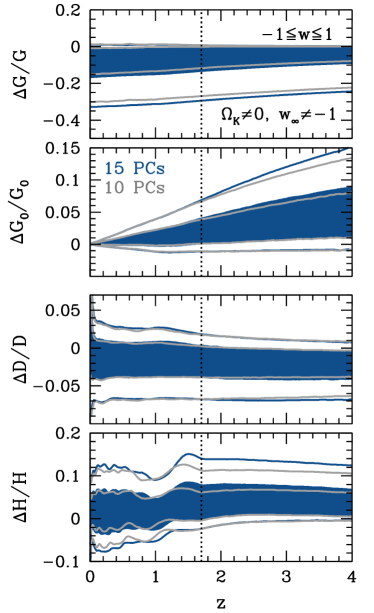
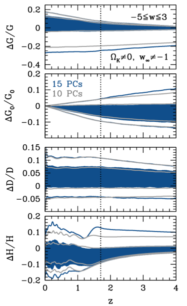
Our basic strategy for determining the number of PCs required for completeness, , is to repeat the MCMC analysis for each class of models using varying numbers of PCs. As we increase the number of components of , we expect the resulting predictions for observables to eventually converge once we have reached the necessary number of PCs. This approach makes the value of to some extent dependent on what we assume about the data and the allowed models. For example, it may be that the component can have a significant effect on certain observables if its amplitude is unconstrained, but limits on this amplitude from the data and/or priors keep the impact of this eigenmode on the observables small. Similarly, it is possible that the value of changes as we add the additional freedom of spatial curvature and early dark energy to the baseline model.
Since our definition of completeness is based on the precision of predictions for a variety of acceleration observables, will generally differ from (and be larger than) the number of dark energy parameters that can be measured to some specified accuracy Linder_Huterer_howmany ; Albrecht_Bernstein ; Suletal07 or the number of parameters required by the data in a Bayesian model selection sense (e.g., Liddle_evidence, ; Davetal07, ).
Figure 23 shows a comparison of observable predictions for the baseline quintessence class (, ), using either 10 or 15 PCs. There is little difference between the two sets of predictions, suggesting that is sufficient for this model class. In contrast, predictions in this class using only 5 PCs are significantly tighter than those with 10 PCs.
Including both curvature and early dark energy in the quintessence model class does not alter the agreement between the predictions for 10 and 15 PCs, as shown in Fig. 24. There is slightly more variation in the limits on observables at , but we do not expect perfect completeness at high redshift anyway due to our simplistic early dark energy parametrization (see below). Even in our most general model class where we weaken the quintessence prior to while continuing to include curvature and early dark energy, as in Fig. 25, the predictions remain robust to increasing the number of PCs from 10 to 15.
These comparisons indicate that is sufficient for completeness in all model classes that we study here. In the main sections of this paper we present results from the larger, “overcomplete” set of 15 PCs.
In our predictions throughout this paper, we have assumed a particular flat CDM model both for PC construction and for creating the fiducial SN and CMB data for MCMC likelihoods. Since the true cosmology could be somewhat different, we can ask how the predictions for observables would change had we assumed a different fiducial model. To test this dependence, we have redone the MCMC analysis using fiducial cosmologies with various values of constant . For simulated SN and CMB data based on (approximately the 68% upper limit of combined constraints on constant from WMAP and current BAO and SN data Komatsu_2008 ), the predictions for growth and expansion observables in the context of quintessence models with either curvature or early dark energy have similar uncertainties to those with a fiducial CDM cosmology (Figs. 6 and 7). The main effect of increasing is that it slightly weakens the impact of the quintessence barrier; moving away from this barrier makes it possible to slightly reduce the dark energy density at from its fiducial level, and therefore the predictions for quintessence models include some features that were previously only allowed in the more general smooth dark energy class. For example, compared with the flat CDM growth history, flat quintessence models with early dark energy are allowed to have at 68% CL instead of , and curved quintessence models with no early dark energy can have at (68% CL) where previously only downward variations in were possible in this class of models. The ability to falsify certain model classes therefore depends on how consistent future SN and CMB data sets are with the standard flat CDM cosmology; any significant variation would be interesting in its own right and would make some changes to the model testing results presented here but not the methodology or the logic of the results themselves.
Another technical issue related to completeness is whether our choice of affects the predictions for observables. This choice enters into both the definition of principal components as discussed in Appendix B and the likelihood for MCMC as the maximum redshift of the fiducial SN sample. To distinguish between the two, let us call the maximum redshift for PCs and for the MCMC likelihood . Note that the choice of also influences our definition of “early dark energy” by setting the minimum redshift at which .
If we keep but extend the PCs to (assuming a flat SN distribution at with the number per bin equal to the number at in the original distribution), the resulting predictions for observables in the flat, no early dark energy quintessence class are similar to those in Fig. 5. The predictions are slightly weaker, particularly at 95% CL, due to the extra freedom in at . The fact that width and redshift dependence of constraints on observables change little with increased indicates that our results are not strongly influenced by the choice of . For example, the tightening of constraints on , , and at high in Fig. 5 is more a consequence of the transition from accelerated expansion to deceleration at than it is of setting .
As another test of sensitivity to , we set as before and also extend the SN distribution for the MCMC analysis to (with constant number per bin at as for the PCs). The resulting predictions for flat quintessence without early dark energy are nearly identical at to the ones in Fig. 5. At lower redshifts, observables are slightly better constrained due to the additional SN data; the largest changes are at , with new 68% limits of and (68% CL). Predictions for growth and expansion observables are relatively insensitive to increasing both and .
At redshifts above our default choice of , we make predictions for observables by specifying through an early dark energy ansatz with a constant equation of state, . While is not a complete parameterization of early dark energy, it does provide guidance for predictions. For example, even though a constant equation of state at is a poor fit to the Albrecht-Skordis model in which a quintessence scalar field has an exponential potential modified by a quadratic polynomial AlbSko00 , as an effective parameter can nevertheless simultaneously fit the CMB distance to the required Planck precision and the growth function at to accuracy. The early dark energy parameterization acts as a diagnostic for whether the dark energy can ever become a substantial fraction of the energy density at given CMB constraints on the distance and energy densities at . Our philosophy is to use an incomplete but representative parameterization that can be used to monitor the need for early dark energy. If a substantial fraction of early dark energy is required by observations under this parameterization, then more complete descriptions and more detailed observations will be required.
References
- (1) A. G. Riess et al., Astron. J. 116, 1009 (1998), [arXiv:astro-ph/9805201].
- (2) S. Perlmutter et al., Astrophys. J. 517, 565 (1999), [arXiv:astro-ph/9812133].
- (3) E. J. Copeland, Dynamics of Dark Energy, in Particles, Strings, and Cosmology-PASCOS 2007, edited by A. Rajantie, C. Contaldi, P. Dauncey and H. Stoica, American Institute of Physics Conference Series Vol. 957, pp. 21–29, 2007, [arXiv:hep-th/0603057].
- (4) E. V. Linder, Reports on Progress in Physics 71, 056901 (2008), [arXiv:0801.2968].
- (5) J. Frieman, M. Turner and D. Huterer, Ann. Rev. Astr. Astrophys. 46, 385 (2008), [arXiv:0803.0982].
- (6) P. M. Garnavich et al., Astrophys. J. 509, 74 (1998), [arXiv:astro-ph/9806396].
- (7) D. N. Spergel et al., Astrophys. J. Suppl. 148, 175 (2003), [arXiv:astro-ph/0302209].
- (8) J. L. Tonry et al., Astrophys. J. 594, 1 (2003), [arXiv:astro-ph/0305008].
- (9) R. A. Knop et al., Astrophys. J. 598, 102 (2003), [arXiv:astro-ph/0309368].
- (10) M. Tegmark et al., Phys. Rev. D69, 103501 (2004), [arXiv:astro-ph/0310723].
- (11) A. G. Riess et al., Astrophys. J. 607, 665 (2004), [arXiv:astro-ph/0402512].
- (12) U. Seljak et al., Phys. Rev. D71, 103515 (2005), [arXiv:astro-ph/0407372].
- (13) D. J. Eisenstein et al., Astrophys. J. 633, 560 (2005), [arXiv:astro-ph/0501171].
- (14) M. Jarvis, B. Jain, G. Bernstein and D. Dolney, Astrophys. J. 644, 71 (2006), [arXiv:astro-ph/0502243].
- (15) A. G. Sanchez et al., Mon. Not. Roy. Astron. Soc. 366, 189 (2006), [arXiv:astro-ph/0507583].
- (16) P. Astier et al., Astron. Astrophys. 447, 31 (2006), [arXiv:astro-ph/0510447].
- (17) D. N. Spergel et al., Astrophys. J. Suppl. 170, 377 (2007), [arXiv:astro-ph/0603449].
- (18) M. Tegmark et al., Phys. Rev. D74, 123507 (2006), [arXiv:astro-ph/0608632].
- (19) A. G. Riess et al., Astrophys. J. 659, 98 (2007), [arXiv:astro-ph/0611572].
- (20) W. M. Wood-Vasey et al., Astrophys. J. 666, 694 (2007), [arXiv:astro-ph/0701041].
- (21) T. M. Davis et al., Astrophys. J. 666, 716 (2007), [arXiv:astro-ph/0701510].
- (22) W. J. Percival et al., Mon. Not. R. Astron. Soc. 381, 1053 (2007), [arXiv:0705.3323].
- (23) L. Guzzo et al., Nature 451, 541 (2008), [arXiv:0802.1944].
- (24) E. Komatsu et al., arXiv:0803.0547.
- (25) M. Kowalski et al., arXiv:0804.4142.
- (26) E. Gaztanaga, A. Cabre and L. Hui, arXiv:0807.3551.
- (27) E. V. Linder and D. Huterer, Phys. Rev. D72, 043509 (2005), [arXiv:astro-ph/0505330].
- (28) D. Sarkar et al., Physical Review Letters 100, 241302 (2008), [arXiv:0709.1150].
- (29) D. Huterer and H. V. Peiris, Phys. Rev. D75, 083503 (2007), [arXiv:astro-ph/0610427].
- (30) S. Chongchitnan and G. Efstathiou, Phys. Rev. D76, 043508 (2007), [arXiv:0705.1955].
- (31) M. Barnard, A. Abrahamse, A. Albrecht, B. Bozek and M. Yashar, Phys. Rev. D78, 043528 (2008), [arXiv:0804.0413].
- (32) M. Tegmark, D. J. Eisenstein, W. Hu and R. G. Kron, arXiv:astro-ph/9805117.
- (33) D. J. Eisenstein, W. Hu and M. Tegmark, Astrophys. J. 518, 2 (1999), [arXiv:astro-ph/9807130].
- (34) A. R. Cooray and D. Huterer, Astrophys. J. 513, L95 (1999), [arXiv:astro-ph/9901097].
- (35) W. Hu, Astrophys. J. 522, L21 (1999), [arXiv:astro-ph/9904153].
- (36) D. Huterer and M. S. Turner, Phys. Rev. D64, 123527 (2001), [arXiv:astro-ph/0012510].
- (37) J. Weller and A. Albrecht, Phys. Rev. D65, 103512 (2002), [arXiv:astro-ph/0106079].
- (38) D. Huterer, Phys. Rev. D65, 063001 (2002), [arXiv:astro-ph/0106399].
- (39) J. Kujat, A. M. Linn, R. J. Scherrer and D. H. Weinberg, Astrophys. J. 572, 1 (2002), [arXiv:astro-ph/0112221].
- (40) I. Maor, R. Brustein, J. McMahon and P. J. Steinhardt, Phys. Rev. D65, 123003 (2002), [arXiv:astro-ph/0112526].
- (41) P. S. Corasaniti and E. J. Copeland, Phys. Rev. D67, 063521 (2003), [arXiv:astro-ph/0205544].
- (42) J. A. Frieman, D. Huterer, E. V. Linder and M. S. Turner, Phys. Rev. D67, 083505 (2003), [arXiv:astro-ph/0208100].
- (43) W. Hu and Z. Haiman, Phys. Rev. D68, 063004 (2003), [arXiv:astro-ph/0306053].
- (44) H.-J. Seo and D. J. Eisenstein, Astrophys. J. 598, 720 (2003), [arXiv:astro-ph/0307460].
- (45) W. Hu and B. Jain, Phys. Rev. D70, 043009 (2004), [arXiv:astro-ph/0312395].
- (46) D. Huterer and A. Cooray, Phys. Rev. D71, 023506 (2005), [arXiv:astro-ph/0404062].
- (47) B. Feng, X.-L. Wang and X.-M. Zhang, Phys. Lett. B607, 35 (2005), [arXiv:astro-ph/0404224].
- (48) S. Wang, J. Khoury, Z. Haiman and M. May, Phys. Rev. D70, 123008 (2004), [arXiv:astro-ph/0406331].
- (49) W. Hu and R. Scranton, Phys. Rev. D70, 123002 (2004), [arXiv:astro-ph/0408456].
- (50) A. Upadhye, M. Ishak and P. J. Steinhardt, Phys. Rev. D72, 063501 (2005), [arXiv:astro-ph/0411803].
- (51) Y. Wang and M. Tegmark, Phys. Rev. D71, 103513 (2005), [arXiv:astro-ph/0501351].
- (52) K. Glazebrook and C. Blake, Astrophys. J. 631, 1 (2005), [arXiv:astro-ph/0505608].
- (53) L. Pogosian, P. S. Corasaniti, C. Stephan-Otto, R. Crittenden and R. Nichol, Phys. Rev. D72, 103519 (2005), [arXiv:astro-ph/0506396].
- (54) M. Sahlen, A. R. Liddle and D. Parkinson, Phys. Rev. D72, 083511 (2005), [arXiv:astro-ph/0506696].
- (55) R. G. Crittenden and L. Pogosian, arXiv:astro-ph/0510293.
- (56) J.-Q. Xia, G.-B. Zhao, B. Feng, H. Li and X. Zhang, Phys. Rev. D73, 063521 (2006), [arXiv:astro-ph/0511625].
- (57) L. Hui and P. B. Greene, Phys. Rev. D73, 123526 (2006), [arXiv:astro-ph/0512159].
- (58) G.-B. Zhao, J.-Q. Xia, X.-M. Zhang and B. Feng, International Journal of Modern Physics D 16, 1229 (2007), [arXiv:astro-ph/0603621].
- (59) L. Knox, Y.-S. Song and H. Zhan, Astrophys. J. 652, 857 (2006), [arXiv:astro-ph/0605536].
- (60) A. Albrecht et al., arXiv:astro-ph/0609591.
- (61) A. R. Liddle, P. Mukherjee, D. Parkinson and Y. Wang, Phys. Rev. D74, 123506 (2006), [arXiv:astro-ph/0610126].
- (62) M. Sahlen, A. R. Liddle and D. Parkinson, Phys. Rev. D75, 023502 (2007), [arXiv:astro-ph/0610812].
- (63) H. Zhan and L. Knox, arXiv:astro-ph/0611159.
- (64) R. Crittenden, E. Majerotto and F. Piazza, Phys. Rev. Lett. 98, 251301 (2007), [arXiv:astro-ph/0702003].
- (65) Y. Wang and P. Mukherjee, Phys. Rev. D76, 103533 (2007), [arXiv:astro-ph/0703780].
- (66) M. Barnard, A. Abrahamse, A. Albrecht, B. Bozek and M. Yashar, Phys. Rev. D77, 103502 (2008), [arXiv:0712.2875].
- (67) A. Abrahamse, A. Albrecht, M. Barnard and B. Bozek, Phys. Rev. D77, 103503 (2008), [arXiv:0712.2879].
- (68) B. Bozek, A. Abrahamse, A. Albrecht and M. Barnard, Phys. Rev. D77, 103504 (2008), [arXiv:0712.2884].
- (69) H. Zhan, L. Knox and J. A. Tyson, arXiv:0806.0937.
- (70) D. Rubin et al., arXiv:0807.1108.
- (71) D. Huterer and M. S. Turner, Phys. Rev. D60, 081301 (1999), [arXiv:astro-ph/9808133].
- (72) A. A. Starobinsky, JETP Lett. 68, 757 (1998), [arXiv:astro-ph/9810431].
- (73) T. Nakamura and T. Chiba, Mon. Not. Roy. Astron. Soc. 306, 696 (1999), [arXiv:astro-ph/9810447].
- (74) T. D. Saini, S. Raychaudhury, V. Sahni and A. A. Starobinsky, Phys. Rev. Lett. 85, 1162 (2000), [arXiv:astro-ph/9910231].
- (75) B. F. Gerke and G. Efstathiou, Mon. Not. Roy. Astron. Soc. 335, 33 (2002), [arXiv:astro-ph/0201336].
- (76) Y. Wang and P. Mukherjee, Astrophys. J. 606, 654 (2004), [arXiv:astro-ph/0312192].
- (77) V. Sahni and A. Starobinsky, Int. J. Mod. Phys. D15, 2105 (2006), [arXiv:astro-ph/0610026].
- (78) C. Li, D. E. Holz and A. Cooray, Phys. Rev. D75, 103503 (2007), [arXiv:astro-ph/0611093].
- (79) C. Zunckel and R. Trotta, Mon. Not. Roy. Astron. Soc. 380, 865 (2007), [arXiv:astro-ph/0702695].
- (80) D. Huterer and G. Starkman, Phys. Rev. Lett. 90, 031301 (2003), [arXiv:astro-ph/0207517].
- (81) W. Hu, Phys. Rev. D66, 083515 (2002), [arXiv:astro-ph/0208093].
- (82) J. Dick, L. Knox and M. Chu, JCAP 0607, 001 (2006), [arXiv:astro-ph/0603247].
- (83) E. V. Linder, Phys. Rev. D70, 061302 (2004), [arXiv:astro-ph/0406189].
- (84) Y. Wang and K. Freese, Phys. Lett. B 632, 449 (2006), [arXiv:astro-ph/0402208].
- (85) G. Aldering et al., arXiv:astro-ph/0405232.
- (86) R. de Putter and E. V. Linder, Astroparticle Physics 29, 424 (2008), [arXiv:0710.0373].
- (87) A. G. Kim, E. V. Linder, R. Miquel and N. Mostek, Mon. Not. R. Astron. Soc. 347, 909 (2004), [arXiv:astro-ph/0304509].
- (88) M. J. Mortonson and W. Hu, Astrophys. J. 672, 737 (2008), [arXiv:0705.1132].
- (89) M. Doran, J.-M. Schwindt and C. Wetterich, Phys. Rev. D64, 123520 (2001), [arXiv:astro-ph/0107525].
- (90) M. Doran and G. Robbers, JCAP 0606, 026 (2006), [arXiv:astro-ph/0601544].
- (91) B. Ratra and P. J. E. Peebles, Phys. Rev. D37, 3406 (1988).
- (92) P. G. Ferreira and M. Joyce, Phys. Rev. D58, 023503 (1998), [arXiv:astro-ph/9711102].
- (93) P. J. Steinhardt, L.-M. Wang and I. Zlatev, Phys. Rev. D59, 123504 (1999), [arXiv:astro-ph/9812313].
- (94) N. Christensen, R. Meyer, L. Knox and B. Luey, Class. Quant. Grav. 18, 2677 (2001), [arXiv:astro-ph/0103134].
- (95) A. Kosowsky, M. Milosavljevic and R. Jimenez, Phys. Rev. D66, 063007 (2002), [arXiv:astro-ph/0206014].
- (96) J. Dunkley, M. Bucher, P. G. Ferreira, K. Moodley and C. Skordis, Mon. Not. R. Astron. Soc. 356, 925 (2005), [arXiv:astro-ph/0405462].
- (97) A. Gelman and D. Rubin, Statistical Science 7, 452 (1992).
- (98) L. Wang and P. J. Steinhardt, Astrophys. J. 508, 483 (1998), [arXiv:astro-ph/9804015].
- (99) E. V. Linder, Phys. Rev. D72, 043529 (2005), [arXiv:astro-ph/0507263].
- (100) Z. Ma, Astrophys. J. 665, 887 (2007), [arXiv:astro-ph/0610213].
- (101) M. Doran, G. Robbers and C. Wetterich, Phys. Rev. D75, 023003 (2007), [arXiv:astro-ph/0609814].
- (102) W. L. Freedman et al., Astrophys. J. 553, 47 (2001), [arXiv:astro-ph/0012376].
- (103) R. R. Caldwell, R. Dave and P. J. Steinhardt, Phys. Rev. Lett. 80, 1582 (1998), [arXiv:astro-ph/9708069].
- (104) M. Chevallier and D. Polarski, Int. J. Mod. Phys. D10, 213 (2001), [arXiv:gr-qc/0009008].
- (105) E. V. Linder, Phys. Rev. Lett. 90, 091301 (2003), [arXiv:astro-ph/0208512].
- (106) C. Armendariz-Picon, V. Mukhanov and P. Steinhardt, Phys. Rev. Lett. 85, 4438 (2000), [arXiv:astro-ph/0004134].
- (107) W. Hu, Astrophys. J. 506, 485 (1998), [arXiv:astro-ph/9801234].
- (108) J. Hamann, S. Hannestad, G. G. Raffelt and Y. Y. Y. Wong, Journal of Cosmology and Astro-Particle Physics 8, 21 (2007), [arXiv:0705.0440].
- (109) W. Hu, ASP Conf. Ser. 339, 215 (2005), [arXiv:astro-ph/0407158].
- (110) J. Kratochvil, A. Linde, E. V. Linder and M. Shmakova, Journal of Cosmology and Astro-Particle Physics 7, 1 (2004), [arXiv:astro-ph/0312183].
- (111) M. Mortonson, W. Hu and D. Huterer, in preparation.
- (112) A. Lewis and S. Bridle, Phys. Rev. D66, 103511 (2002), [arXiv:astro-ph/0205436].
- (113) D. Huterer and E. V. Linder, Phys. Rev. D75, 023519 (2007), [arXiv:astro-ph/0608681].
- (114) E. V. Linder and R. N. Cahn, Astroparticle Physics 28, 481 (2007), [arXiv:astro-ph/0701317].
- (115) D. Polarski and R. Gannouji, Phys. Lett. B 660, 439 (2008), [arXiv:0710.1510].
- (116) V. Acquaviva, A. Hajian, D. N. Spergel and S. Das, Phys. Rev. D78, 043514 (2008), [arXiv:0803.2236].
- (117) M. J. White and C. S. Kochanek, Astrophys. J. 560, 539 (2001), [arXiv:astro-ph/0105227].
- (118) A. I. Vainshtein, Phys. Lett. B39, 393 (1972).
- (119) W. Hu and I. Sawicki, Phys. Rev. D76, 104043 (2007), [arXiv:0708.1190].
- (120) H. Oyaizu, M. Lima and W. Hu, arXiv:0807.2462.
- (121) B. A. Bassett and M. Kunz, Phys. Rev. D69, 101305 (2004), [arXiv:astro-ph/0312443].
- (122) J.-P. Uzan, N. Aghanim and Y. Mellier, Phys. Rev. D70, 083533 (2004), [arXiv:astro-ph/0405620].
- (123) Y.-S. Song and W. Hu, Phys. Rev. D73, 023003 (2006), [arXiv:astro-ph/0508002].
- (124) C. Clarkson, B. Bassett and T. H.-C. Lu, Phys. Rev. Lett. 101, 011301 (2008), [arXiv:0712.3457].
- (125) E. V. Linder and D. Huterer, Phys. Rev. D67, 081303 (2003), [arXiv:astro-ph/0208138].
- (126) M. Kunz, arXiv:astro-ph/0702615.
- (127) A. Albrecht and G. Bernstein, Phys. Rev. D75, 103003 (2007), [arXiv:astro-ph/0608269].
- (128) A. Albrecht and C. Skordis, Physical Review Letters 84, 2076 (2000), [arXiv:astro-ph/9908085].