Percolation on correlated networks

Abstract

We reconsider the problem of percolation on an equilibrium random network with degree–degree correlations between nearest-neighboring vertices focusing on critical singularities at a percolation threshold. We obtain criteria for degree–degree correlations to be irrelevant for critical singularities. We present examples of networks in which assortative and disassortative mixing leads to unusual percolation properties and new critical exponents.

I Introduction

Real-world networks are correlated ab01a ; dm01c ; pvv01 ; Newman:n03a ; blm06 . Correlations between degrees of vertices in a network essentially characterise its structure. Various real-world networks are markedly different in respect of degree-degree correlations pvv01 ; vpv02 ; Maslov:ms02 ; Maslov:msz02 ; Newman:n02 . In particular, social networks show assortative mixing, i.e., a preference of high-degree vertices to be connected to other high-degree vertices, while technological and biological networks are mostly disassortative, i.e., their high-degree vertices tend to be connected to low-degree ones Newman:n02 . However, even the simplest correlated networks with only pair correlations between the nearest-neighbor degrees are still poorly understood. Our aim is to find when the critical singularities for correlated networks of this kind coincide with those for well-studied uncorrelated networks and when and how much they differ.

At the present time it is well established that the small-world effect and heterogeneity influence the cooperative dynamics and critical phenomena of models defined on the top of complex networks Dorogovtsev:dgm07 . However, numerous studies were devoted mostly to more simple, uncorrelated networks. In an uncorrelated network with a heavy-tailed degree distribution, critical singularities of a continuous phase transition are characterized by model dependent critical exponents which differ from the standard mean-field ones and the critical exponents of two and three dimensional lattices, see, for example, Refs. g89 ; sa03 ; b06 . The critical behavior depends on an asymptotic behavior of a degree distribution at large degrees. For percolation on an uncorrelated complex network that was demonstrated in cah02 ; cha03 . One should expect, however, that for dynamical processes taking place in a complex networks, correlations are important. The simplest particular kind of correlations in a networks are correlations between degrees of two nearest neighbors in a network—so called degree–degree correlations. In this work we consider only these specific, though representative, correlations. Investigations of percolation Newman:n02 ; Vazquez:vm03 and epidemic spreading Boguna:bp-s02 ; Boguna:bpv03 demonstrated that the degree–degree correlations strongly influence these phenomena. The birth and growth of the giant connected component significantly depends on the type of correlations—whether the degree–degree correlations are assortative or disassortative. Compared to an uncorrelated network with the same degree distribution, the assortative correlations increase the resilience of a network against random damage, while the disassortative correlations diminish this resilience.

Figure 1: Schematic representation of eigenvalues (crosses) of the branching matrix, Eq. (4), in the limit $N\rightarrow\infty$. There are four situations: (a) the largest eigenvalue $\lambda_{1}$ is nonzero while all other eigenvalues are zero, $\lambda_{i}=0$ for $i\geq 2$; (b) both the largest eigenvalue $\lambda_{1}$ and the second largest eigenvalue $\lambda_{2}$ are finite; (c) $\lambda_{1}$ diverges but $\lambda_{2}$ is finite; (d) the sequence of eigenvalues is unbounded. Case (a) takes place for uncorrelated networks but also can occur in specific disassortative networks. Cases (b)-(d) occur only in correlated networks.

Table 1: Critical behavior of the order parameter $y\propto(p-p_{c})^{\beta}$, where $p$ is an occupation probability, in correlated networks with a degree distribution $P(q)\sim q^{-\gamma}$. $\lambda_{1}$ and $\lambda_{2}$ are the largest and second largest eigenvalues of the branching matrix, Eq. (4). “Weakly” correlated networks, both assortative and disassortative, have the same critical behavior as uncorrelated network with the identical degree distribution, e.i., correlations are irrelevant. Model (44) with assortative mixing has a new critical exponent $\beta$ in the range $-1<\alpha\leq 0$. Here, the parameter $\alpha$ determines the average degree of the nearest neighbor of a vertex with $q$ connections: $\overline{q}_{nn}(q)=\text{const}+q^{-\alpha}$. At $\alpha>0$ this model is “weakly” correlated. Model (62) with disassortative mixing has a new critical behavior at $\alpha>0$. For this model, $\overline{q}_{nn}(q)=1+q^{-\alpha}$. The $(\gamma,\alpha)$ phase diagrams of models (44) and (62) are shown in Figs. 5 and 6, respectively.

Network	$\gamma$	Region on	$\lambda$	$p_{c}=1/\lambda_{1}$	$\beta$
		$(\gamma,\alpha)$ plane
uncorrelated or	$\gamma>4$		$\lambda_{1},\lambda_{2}<\infty$	$>0$	1
“weakly” correlated	$3<\gamma<4$		$\lambda_{1},\lambda_{2}<\infty$	$>0$	$1/(\gamma-3)$
	$2<\gamma<3$		$\lambda_{1}=\infty,\lambda_{2}<\infty$	0	$1/(3-\gamma)$
strongly assortative	$\gamma>3+\alpha$	I	$\lambda_{1},\lambda_{2}=\infty$	0	$(2-\gamma+\alpha)/\alpha$
	$2<\gamma<3+\alpha$	II	$\lambda_{1},\lambda_{2}=\infty$	0	$1/(3-\gamma)$
strongly disassortative	$\gamma>4-3\alpha$	I	$\lambda_{1}<\infty,\,\,\,\lambda_{2}=0$	$>0$	1
	$3-2\alpha<\gamma<4-3\alpha$	II	$\lambda_{1}<\infty,\,\,\,\lambda_{2}=0$	$>0$	$(1-\alpha)/(\gamma-3+2\alpha)$
	$2<\gamma<3-2\alpha$	III	$\lambda_{1}=\infty,\,\,\,\lambda_{2}=0$	0	$(1-\alpha)/(3-\gamma-2\alpha)$

One can construct an equilibrium network, where only degree–degree correlations are present—the maximally random network with given degree–degree correlations. This is impossible for non-equilibrium, in particular, growing networks. Growing networks necessarily demonstrate a wide spectrum of correlations and not only pair correlations between degrees of the nearest neighbors. This type of heterogeneity may result in an anomalous critical effect at the birth point of a giant connected component Callaway:chk01 ; Dorogovtsev:dms01b ; kr02 ; l02 ; kkkr02 ; bb03 ; cb03 ; kd04 . This transition resembles the Berezinskii-Kosterlitz-Thouless phase transition in condensed matter Berezinskii:b70 ; Kosterlitz:kt73 . The transition is explained by a specific large-scale inhomogeneity of non-equilibrium networks and related correlations. The large-scale inhomogeneity here means the difference in properties of vertices according to age kr01 ; bp-s05 .

One should note that degree–degree correlations may also arise in an equilibrium network if self-loops and multiple connections are forbidden. In particular, this was demonstrated in Ref. lgkk06 for the static model of scale-free networks Goh:gkk01 . Noh Noh:n07 observed an unusual critical behavior in an exponential random graph model with a tunable degree–degree correlations.

The earlier investigations Newman:n02 ; Vazquez:vm03 ; Boguna:bp-s02 ; Boguna:bpv03 mostly focused on the effect of degree–degree correlations on the percolation and epidemic thresholds. In the present paper we investigate the effect of degree–degree correlations in equilibrium networks on critical singularities at the percolation threshold. We demonstrate that the critical behavior is determined by the spectrum of a so-called branching matrix and a degree distribution. The eigenvalues of this matrix are real and can be ordered in descending order. The largest eigenvalue determines the percolation threshold and can be both finite and infinite depending on a degree distribution in agreement with Refs. Newman:n02 ; Vazquez:vm03 . We derive necessary and sufficient conditions for degree–degree correlations to be irrelevant for critical singularities. We give examples of strongly correlated networks with assortative and disassortative mixing in which at least one of these conditions is not fulfilled. These networks demonstrate new critical singularities, see Table 1. In particular, we propose analytically treatable assortative networks with an unbounded sequence of eigenvalues in the infinite size limit and show that this peculiarity of the spectrum leads to a new critical behavior. Remarkably, this network may be robust against a random damage even if the second moment of its degree distribution is finite. This is in contrast to uncorrelated networks which are robust only if the second moment of a degree distribution diverges. We also study specific disassortative networks which demonstrate new critical singularities and are fragile. Remarkably, this takes place despite the second moment of their degree distribution may be divergent and the largest eigenvalue is finite. Our results are summed up in Table 1 and Figs. 5 and 6 which display phase diagrams of two model networks with strong assortative and disassortative mixing.

The paper is organized as follows. In Sec. II we give a general description of correlations in a network and introduce the branching matrix. In Sec. III we introduce a basic equation describing percolation on a degree–degree correlated network and reconsider the effect of assortative and disassortative mixing on the percolation threshold. In Sec. IV we find criteria for degree–degree correlations to be irrelevant for critical singularities. Sec. V introduces a simple model of degree–degree correlated networks which have a modular structure and an unbounded sequence of eigenvalues of the branching matrix. In Sec. VI we demonstrate that these networks have new critical singularities. Disassortative networks with unusual critical properties are studied in Sec. VII. A detailed analysis of the spectrum, its relationships with structural coefficients of a correlated network and calculation of the entropy of the model network are presented in Appendices A, B and C, respectively.

II Degree–degree correlations

We consider a random locally tree-like network of $N$ vertices in which only pair correlations between nearest neighbor degrees $q$ and $q^{\prime}$ are present. We assume that there are vertices with degrees $q=q_{1},q_{2},...q_{cut}$, and in total there are $N_{d}$ different values of degrees. This correlated network is completely described by a given symmetric joint degree-degree distribution, $P(q,q^{\prime})=P(q^{\prime},q)$, otherwise the network is homogeneously random. The degree distribution $P(q)$ can be calculated from $P(q,q^{\prime})$ as follows:

$$\sum_{q^{\prime}}P(q^{\prime},q)=qP(q)/\langle q\rangle,$$ (1)

where the brackets $\langle...\rangle$ denote an average over the degree distribution $P(q)$, for example, $\langle q\rangle=\sum_{q}qP(q)$. Below for brevity we use the notations: $z_{1}\equiv\langle q\rangle$ and $z_{2}\equiv\langle q(q-1)\rangle$. It is convenient to introduce the conditional probability,

$$P(q^{\prime}|q)=\frac{z_{1}P(q,q^{\prime})}{qP(q)},$$ (2)

that if an end vertex of an edge has degree $q$, then the second end has degree $q^{\prime}$. The functions $P(q,q^{\prime})$ and $P(q^{\prime}|q)$ are normalized:

$$\sum_{q,q^{\prime}}P(q,q^{\prime})=\sum_{q^{\prime}}P(q^{\prime}|q)=1.$$ (3)

In uncorrelated networks the conditional probability does not depend on $q$: $P(q^{\prime}|q)=q^{\prime}P(q^{\prime})/z_{1}$. We define a non-symmetric branching matrix as follows:

$$B_{qq^{\prime}}=(q^{\prime}-1)P(q^{\prime}|q).$$ (4)

This matrix has the following property:

$$q(q-1)P(q)B_{qq^{\prime}}=q^{\prime}(q^{\prime}-1)P(q^{\prime})B_{q^{\prime}q}.$$ (5)

According to definition (4), an entry $B_{qq^{\prime}}$ of this matrix is equal to the branching coefficient $q^{\prime}-1$ of an edge, which emanates from a vertex with degree $q$ and has a vertex with degree $q^{\prime}$ at the second end, multiplied by the probability $P(q^{\prime}|q)$ that the second end has degree $q^{\prime}$. In Secs. III and IV we will show that the structure of the spectrum of this matrix determines the critical properties of the percolation. Relationship of this spectrum with clustering coefficients and the mean intervertex distance in a correlated network is considered in Appendix B.

Using the branching matrix we can calculate the average branching coefficient $B(q)$ of an edge which emanates from a vertex of degree $q$:

$$B(q)=\sum_{q^{\prime}}B_{qq^{\prime}}.$$ (6)

The coefficient $B(q)$ is related to the average nearest-neighbor’s degree of the vertices of degree $q$:

$$\overline{q}_{nn}(q)=\sum_{q^{\prime}}q^{\prime}P(q^{\prime}|q)=B(q)+1.$$ (7)

A mean branching coefficient $\overline{B}$ is equal to

$$\overline{B}=\frac{1}{z_{1}}\sum_{q}B(q)qP(q)=\frac{z_{2}}{z_{1}}=\frac{\langle q^{2}\rangle}{\langle q\rangle}-1.$$ (8)

It only depends on the degree distribution $P(q)$. An integral characteristic of degree-degree correlations is given by the Pearson coefficient Newman:n02 :

$$r=\frac{1}{z_{1}\sigma^{2}}\sum_{q}[B(q)-\overline{B}]q(q-1)P(q),$$ (9)

where

$$\sigma^{2}{=}\sum_{q}(q{-}1)^{2}\,\frac{qP(q)}{z_{1}}\,-\left[\sum_{q}(q{-}1)\frac{qP(q)}{z_{1}}\right]^{2}\!\!\!\!=\!\frac{\langle q^{3}\rangle}{\langle q\rangle}{-}\frac{\langle q^{2}\rangle^{2}}{\langle q\rangle^{2}}$$

is for normalization. The Pierson coefficient is positive for assortative mixing and negative for disassortative mixing.

In an uncorrelated complex network, $\overline{q}_{nn}(q)$ does not depend on $q$: $\overline{q}_{nn}(q)=\overline{B}+1$. In contrast, in networks with assortative mixing, $\overline{q}_{nn}(q)$ increases with increasing $q$ while in disassortative networks it decreases. For example, $\overline{q}_{nn}(q)$ shows a power law decay $\overline{q}_{nn}(q)\propto q^{-0.5}$ for the Internet pvv01 ; vpv02 . Recursive scale-free networks, growing by the linear preferential attachment mechanism, have growing asymptotics $\overline{q}_{nn}(q)\sim\ln q$ at large $q$ at $\gamma>3$ and decaying $\overline{q}_{nn}(q)$ as a power law at $2<\gamma<3$ bp-s05 ; kr02 .

III Tree ansatz equations and percolation threshold

A key quantity in the percolation problem is the probability $x_{q}$ that if an edge is attached to a vertex of degree $q$, then, following this edge to its second end, we will not appear in a giant connected component Vazquez:vm03 . The number of unknown order parameter components $x_{q}$ is equal to the number of different degrees, $N_{d}$. In contrast, only a one-component order parameter $x$ describes percolation on an uncorrelated complex network Callaway:cns00 ; nsw01 .

Let $p$ be the probability that a vertex is retained in a randomly damaged network. Within a tree-ansatz theory, which assumes that a network has a locally tree-like structure, equations for the probabilities $x_{q}$ and the relative size $S$ of a giant connected component have the following form Vazquez:vm03 :

$$x_{q}=1-p+p\sum_{q^{\prime}}P(q^{\prime}|q)(x_{q^{\prime}})^{q^{\prime}-1},$$ (10)

$$1-S=1-p+p\sum_{q}P(q)(x_{q})^{q}.$$ (11)

Equations (10) and (11) directly generalize equations derived for percolation on an uncorrelated complex network Callaway:cns00 ; nsw01 , where $x_{q}=x$, see also Refs. dm01c ; Newman:n03a ; Dorogovtsev:dgm07 . The set of Eqs. (10) determines unknown probabilities $x_{q}$ for $q=q_{1},q_{2},...q_{cut}$. Newman Newman:n02 originally derived these equations using generating functions, and numerically solved them for various networks. The analysis of Eqs. (10) shows that the birth of the giant connected component is a continuous phase transition. Below the percolation threshold, i.e., at $p<p_{c}$, these equations only have a trivial solution $x_{q}=1$, and there is no giant connected component. A giant connected component is present above the percolation point, $p>p_{c}$, where there is a solution with $x_{q}<1$. Introducing a parameter $y_{q}=1-x_{q}$, we rewrite Eq. (10) as follows:

$$p\sum_{q^{\prime}}B_{qq^{\prime}}y_{q^{\prime}}-y_{q}=p\sum_{q^{\prime}=3}^{q_{cut}}\sum_{n=2}^{q^{\prime}-1}{q^{\prime}-1\choose n}(-y_{q^{\prime}})^{n}P(q^{\prime}|q).$$ (12)

One can solve this set of equations near the critical point, $\tau=p/p_{c}-1\ll 1$ when $y_{q}\ll 1$.

First we study the percolation threshold for a degree–degree correlated network. We will use the spectral properties of the branching matrix, Eq. (4), so let us remind some basics. Eigenvalues $\lambda_{i}$ and eigenvectors $\Phi^{(i)}_{q}$ associated with these eigenvalues are defined by the equation:

$$\sum_{q^{\prime}}B_{qq^{\prime}}\Phi_{q^{\prime}}^{(i)}=\lambda_{i}\Phi_{q}^{(i)},$$ (13)

where the index $i$ labels the eigenvalues, $i=1,2,\ldots,N_{d}$. We consider the case of positive entries: $B_{qq^{\prime}}>0$. The following statements hold. (i) The largest eigenvalue $\lambda_{1}$ is positive. (ii) The entries $\Phi_{q}^{(1)}$ of the maximal eigenvector are positive, $\Phi_{q}^{(1)}>0$. (iii) All eigenvalues $\lambda_{i}$ are real and can be ordered: $\lambda_{1}>\lambda_{2}>...>\lambda_{N_{d}}$. (iv) The eigenvectors $\Phi^{(i)}$ associated with these eigenvalues form a complete orthonormal basis set. That is,

$$\sum_{q}w(q)\Phi_{q}^{(i)}\Phi_{q}^{(j)}=\delta_{i,j},$$ (14)

$$w(q)\sum_{\lambda}\Phi_{q}^{(\lambda)}\Phi_{q^{\prime}}^{(\lambda)}=\delta_{q,q^{\prime}},$$ (15)

where $w(q)=q(q-1)P(q)/z_{1}$ is a weight function, $\delta_{i,j}$ and $\delta_{q,q^{\prime}}$ are the Kronecker symbols. Properties (i) and (ii) follows from the Perron-Frobenius theorem, see, for example, Ref. Minc . Properties (iii) and (iv) are proved in Appendix A. One can show that for an uncorrelated network there is a single largest eigenvalue and an ($N_{d}-1$)-degenerate zero eigenvalue:

$$\lambda_{1}=z_{2}/z_{1},\,\,\,\,\lambda_{i\geq 2}=0.$$ (16)

The percolation threshold corresponds to a critical probability $p_{c}$ above which a nontrivial solution of Eq. (12), $y_{q}\geq 0$, appears. Taking into account only the linear terms, we get the following condition:

$$y_{q}=p\sum_{q^{\prime}}B_{qq^{\prime}}y_{q^{\prime}}.$$ (17)

We represent $y_{q}$ as a linear combination of the mutually orthogonal eigenvectors which we call modes:

$$y_{q}=\sum_{i=1}^{N_{d}}a_{i}\Phi_{q}^{(i)}.$$ (18)

The amplitudes $a_{i}$ are unknown functions of $p$. It is obvious that $a_{i}=0$ at $p<p_{c}$. Substituting Eq. (18) into Eq. (17) and using the orthogonality Eq. (14) of the eigenvectors, we obtain an equation $a_{i}=p\lambda_{i}a_{i}$. One can see that a nontrivial solution $a_{1}\neq 0$ appears when $p\lambda_{1}=1$. So the mode associated with $\lambda_{1}$ is critical. This gives the following criterion for the percolation threshold found in Refs. Newman:n02 ; Vazquez:vm03 :

$$p_{c}\lambda_{1}=1.$$ (19)

Thus the generalization of the Molloy–Reed criterion to undamaged correlated networks, i.e., at $p=1$, is the following condition: if the largest eigenvalue $\lambda_{1}$ of the branching matrix, $B_{qq^{\prime}}$, is larger than $1$, then the correlated network has a giant connected component. In uncorrelated networks the criterion (19) is reduced to the well-known one: $z_{2}/z_{1}=1$.

In Appendix A we prove that at a given degree distribution $P(q)$, the largest eigenvalue $\lambda_{1}^{(as)}$ of an assortative network is larger then $z_{2}/z_{1}$ while in a disassortative network it is smaller:

$$\lambda_{1}^{(dis)}<\frac{z_{2}}{z_{1}}<\lambda_{1}^{(as)}.$$ (20)

There are the following lower and upper boundaries for $\lambda_{1}$ (see Appendix A):

$$\frac{1}{z_{2}}\sum_{q}B(q)q(q-1)P(q)\leq\lambda_{1}\leq\max_{q}B(q).$$ (21)

Suppose that a degree distribution is such that $z_{2}/z_{1}=1$. Then inequality (20) leads to the following statements. (i) An uncorrelated network with this degree distribution is at the birth point of a giant connected component. (ii) An assortative network with this degree distribution has a giant connected component. (iii) A disassortative network with this degree distribution has no giant connected component. According to criterion (19) and inequality (20), percolation thresholds in randomly damaged assortative and disassortative networks with the same degree distribution satisfy the inequality:

$$p_{c}^{(as)}<z_{1}/z_{2}<p_{c}^{(dis)}.$$ (22)

Therefore, assortative mixing enhances resilience of a correlated network against random damage while a disassortative mixing decreases it Newman:n02 .

If the largest eigenvalue $\lambda_{1}$ diverges in the infinite network, then the percolation threshold $p_{c}$ tends to zero. In this case the giant connected component of a correlated network cannot be eliminated by a random removal of vertices Vazquez:vm03 . In an assortative network, in accordance with inequality (20), this takes place when the second moment $z_{2}$ diverges. This criterion ($z_{2}\to\infty$) of the robustness of an uncorrelated network was found in Albert:ajb00 ; cah02 . Remarkably, $\lambda_{1}$ can diverge even if an assortative network has a finite $z_{2}$ but degree–degree correlations are sufficiently strong. An example of an assortative network of this kind is given in Sec. V. On the other hand, Vaázquez and Moreno Vazquez:vm03 found a network with strong disassortative mixing, which has a finite percolation threshold and is fragile against a random damage even if the second moment $z_{2}$ diverges.

IV Critical behavior of “weakly” correlated networks

In this section we derive necessary and sufficient conditions for degree–degree correlations to be irrelevant for critical singularities at the percolation transition. These conditions are:

• The largest eigenvalue $\lambda_{1}$ of the branching matrix must be finite if $\langle q^{2}\rangle$ is finite, or $\lambda_{1}\rightarrow\infty$ if $\langle q^{2}\rangle\rightarrow\infty$.

• The second largest eigenvalue $\lambda_{2}$ must be finite.

• A sequence of entries $\Phi_{q}^{(1)}$ of the maximum eigenvector of this matrix must converge to a finite non-zero value at $q\rightarrow\infty$, see Eq. (30).

Let us solve Eq. (12) near the percolation transition. We use the fact that the eigenvectors $\Phi_{q}^{(i)}$ of the branching matrix $\widehat{B}$ form the complete orthogonal basis set, see Eqs. (14) and (15). Substituting Eq. (18) into Eq. (12), we get a set of nonlinear equations for unknown amplitudes $a_{i}$:

$$(p\lambda_{i}-1)a_{i}=p\lambda_{i}S_{i}(\textbf{a}).$$ (23)

Here $S_{i}(\textbf{a})$ is a function of the amplitudes $\textbf{a}=(a_{1},a_{2},...)$:

$$S_{i}(\textbf{a})=\frac{1}{z_{1}}\sum_{q=3}^{q_{cut}}\sum_{n=2}^{q-1}{q-1\choose n}(-y_{q})^{n}qP(q)\Phi_{q}^{(i)}.$$ (24)

Let us find $a_{i}$ in the leading order in $\tau\ll 1$ under conditions I and II. Substituting Eq. (18) into Eqs. (23) and (24) and taking into account only the quadratic terms in $a_{i}$, we get a set of approximate equations for the amplitudes $a_{i}$:

$$(p\lambda_{i}-1)a_{i}=p\lambda_{i}\sum_{m,n}M_{imn}a_{m}a_{n},$$ (25)

where

$$M_{imn}=\frac{1}{2z_{1}}\sum_{q}q(q-1)(q-2)P(q)\Phi_{q}^{(i)}\Phi_{q}^{(n)}\Phi_{q}^{(m)}.$$ (26)

Let us first consider a degree–degree correlated network with finite coefficients $M_{imn}$ in the infinite size limit $N\rightarrow\infty$. In the leading order in $\tau$, equation (25) has a solution

$$a_{1}\simeq\frac{\tau}{M_{111}}+O(\tau^{2}),$$ (27)

$$a_{i}\simeq-\frac{\lambda_{i}a_{1}^{2}M_{i11}}{(\lambda_{1}-\lambda_{i})}\propto O(\tau^{2})\ \ \ \text{for $i\geq 2$}.$$ (28)

One can see that the amplitude $a_{1}$ of the critical mode $\lambda_{1}$ has the standard mean-field dependence. It is much larger than the amplitudes $a_{i}$ of the modes $i\geq 2$ which we call transverse modes. Therefore near the percolation threshold the order parameter $y_{q}=1-x_{q}$ is mainly determined by the critical mode $\Phi_{q}^{(1)}$ associated with the largest eigenvalue. The transverse modes give a smaller contribution:

$$y_{q}\approx a_{1}\Phi_{q}^{(1)}+O(a_{1}^{2}).$$ (29)

Above we assumed that the coefficient $M_{111}$ is finite. This assumption takes place if the sequence of entries $\Phi_{q}^{(1)}$ converges at $q\rightarrow q_{cut}\rightarrow\infty$, e.i., $\lim_{q\rightarrow\infty}\Phi_{q}^{(1)}<\infty$. If this limiting value is non-zero,

$$0<\lim_{q\rightarrow\infty}\Phi_{q}^{(1)}<\infty,$$ (30)

then the third moment $\langle q^{3}\rangle$ of the degree distribution must be finite, $\langle q^{3}\rangle<\infty$. Equation (30) is the condition III formulated above. Thus we conclude that under conditions I–III the percolation in a correlated scale-free networks with $\gamma>4$ has the standard mean-field critical behavior, Eq. (27), with the critical exponent $\beta=1$. In Sec. VII we will show that the case $\lim_{q\rightarrow\infty}\Phi_{q}^{(1)}=0$, e.i., the condition III is broken down, corresponds to a strongly correlated network.

Consider the case $3<\gamma\leq 4$ under conditions I–III. In this case it is necessary to take into account all orders in $a_{1}$ in Eq. (23). The reason is that the coefficients of the expansion over $a_{1}$ diverge as $N\rightarrow\infty$. It is this divergence that leads to the non-standard critical behavior of percolation on an uncorrelated complex network cah02 ; cha03 . We assume that the inequality $a_{1}\gg a_{i}$ for all $i\geq 2$ is also valid at $3<\gamma\leq 4$. Below we will confirm this assumption. We expand the function $S_{i}(\textbf{a})$ over the amplitudes $a_{i}$ of the transverse modes and save only linear terms in $a_{i}$:

$$S_{i}(\textbf{a})\simeq s_{i}(a_{1})+\sum_{j\geq 2}s_{ij}(a_{1})a_{j}+...,$$ (31)

where

$$s_{i}(a_{1})\equiv S_{i}(a_{1},0,0,\ldots),$$ (32)

$$s_{ij}(a_{1})\equiv\frac{\partial S_{i}(\textbf{a})}{\partial a_{j}}|_{\textbf{a}=(a_{1},0,0,..)}.$$ (33)

The function $s_{i}(x)$ is given by the following series:

$$s_{i}(x)=\sum_{n=2}^{{}^{q_{cut}-1}}K_{i}(n)(-x)^{n},$$ (34)

where

$$K_{i}(n)=\frac{1}{z_{1}}\sum_{q=n+1}^{q_{cut}}{q-1\choose n}qP(q)(\Phi_{q}^{(1)})^{n}\Phi_{q}^{(i)}.$$ (35)

Similarly, the function $s_{ij}(x)$ is

$$s_{ij}(x)=\sum_{n=2}^{{}^{q_{cut}-1}}K_{ij}(n)(-x)^{n},$$ (36)

$$\!\!\!\!\!\!\!\!\!\!\!\!\!\!\!\!\!K_{ij}(n)=\frac{n}{z_{1}}\!\sum_{q=n+1}^{q_{cut}}{q-1\choose n}qP(q)(\Phi_{q}^{(1)})^{n-1}\Phi_{q}^{(i)}\Phi_{q}^{(j)}.$$ (37)

At $3<\gamma\leq 4$ the functions $s_{i}(x)$ and $s_{ij}(x)$ are singular functions of $x$ because the coefficients $K_{i}(n)$ and $K_{ij}(n)$ diverge as $q_{cut}(N)\rightarrow\infty$. Using the method of summation used in cah02 ; Goltsev:gdm03 we get asymptotic results:

$$s_{i}(x)\approx b_{i}x^{\gamma-2},$$

$$s_{ij}(x)\approx b_{ij}x^{\gamma-3}.$$ (38)

Here the numerical coefficients $b_{i}$ and $b_{ij}$, where $i,j=1,2,...\,$, depend on a specific model of a correlated network. Substituting Eqs. (24) and (38) into Eq. (23) we obtain a set of nonlinear equations

$$(p\lambda_{i}-1)a_{i}=p\lambda_{i}[b_{i}a_{1}^{\gamma-2}+a_{1}^{\gamma-3}\sum_{j\geq 2}b_{ij}a_{j}]$$ (39)

for $i=1,2,...\,$. They have an asymptotic solution

$$a_{1}\approx\Bigl{(}\frac{\tau}{b_{1}}\Bigr{)}^{1/(\gamma-3)},$$ (40)

$$a_{i}\approx-\frac{b_{i}\lambda_{i}a_{1}^{\gamma-2}}{(\lambda_{1}-\lambda_{i})}\propto O(\tau^{(\gamma-2)/(\gamma-3)}).$$ (41)

In the case $3<\gamma\leq 4$ the amplitude $a_{1}$ of the critical mode $\Phi_{q}^{(1)}$ also is mush larger than the amplitudes of the transverse modes, i.e., $a_{1}\gg a_{i}$ for all $i\geq 2$. So, in the leading order, we get $y_{q}\approx a_{1}\Phi_{q}^{(1)}$. The critical exponent $\beta$ is equal to $1/(\gamma-3)$ as for an uncorrelated network with the identical degree distribution.

Now consider the case $2<\gamma\leq 3$ under conditions (I)–(III). According to Eq. (20), in an assortative network with a divergent second moment $z_{2}$ the largest eigenvalue $\lambda_{1}$ diverges in the limit $N\rightarrow\infty$. The percolation threshold is $p_{c}=0$, and a giant connected component is present at any $p>0$. One can show that at $p\ll 1$ the order parameter $y_{q}$ and the size of giant connected component $S$ are

$$y_{q}\propto p^{\beta}\Phi_{q}^{(1)},$$ (42)

$$S\propto p^{1+\beta}$$ (43)

where $\beta=1/(3-\gamma)$. This is the same singularity as was found in uncorrelated networks with $2<\gamma<3$ cah02 ; cha03 . This result is also valid for disassortative networks with $\lambda_{1}=\infty$.

The main conclusion of this section is that under conditions (I)–(III), a correlated complex network has the same critical behavior as an uncorrelated random network with the identical degree distribution. Our results are summed up in Table 1.

Degree-degree correlations may be strong and violate one of these conditions. In Sec. VI and Sec. VII we will give examples of such networks and new critical singularities.

V Exactly solvable model of a correlated network

In this section we introduce a simple model of a correlated network which allows analytical treatment. This, actually, toy model permits us to check general results of the percolation theory derived above and to study an effect of strong assortative mixing. This model is also interesting due to its clear modular structure.

Let us consider a correlated network with a given degree distribution $P(q)$ and a degree-degree distribution $P(q,q^{\prime})$ which is factorized at $q\neq q^{\prime}$ as follows:

$$P(q,q^{\prime})=\delta_{q,q^{\prime}}[f(q)+1]\rho^{2}(q)P^{2}(q)$$

$$+(1-\delta_{q,q^{\prime}})\rho(q)P(q)\rho(q^{\prime})P(q^{\prime}).$$ (44)

Compare this with an uncorrelated network where $P(q,q^{\prime})=qP(q)q^{\prime}P(q^{\prime})/z_{1}^{2}$ which corresponds to $\rho(q)=q/z_{1}$. The function $f(q)$ is non-negative for assortative mixing. In this case vertices at the ends of an edge have the same degree with a higher probability rather than different degrees. In the limit $f(q)\rightarrow\infty$ we have a set of disconnected random $q$-regular modules. For disassortative mixing, we choose $-1<f(q)\leq 0$, then the probability to have different degrees at the ends of an edge is higher than to have the same degree.

For a given degree distribution $P(q)$ and a function $f(q)$, the substitution of Eq. (44) into Eq. (1) gives the following equation for the function $\rho(q)$:

$$\rho(q)=\frac{q}{z_{1}\rho}\frac{2}{1+[1+4qf(q)P(q)/(z_{1}\rho)]^{1/2}},$$ (45)

where the parameter $\rho$ must be found self-consistently from the equation:

$$\rho=\sum_{q}\rho(q)P(q).$$ (46)

For model (44), eigenvalues $\lambda$ and eigenvectors $\Phi^{(\lambda)}_{q}$ of the branching matrix, Eq. (4), are determined by the following exact equations:

$$1=z_{1}\sum_{q}\frac{(q-1)}{q}\frac{\rho^{2}(q)P(q)}{\lambda-\Lambda(q)},$$ (47)

$$\Phi^{(\lambda)}_{q}=\frac{z_{1}\rho(q)n(\lambda)}{q[\lambda-\Lambda(q)]}.$$ (48)

Here we have introduced a function

$$\Lambda(q)=\frac{(q-1)}{q}z_{1}f(q)\rho^{2}(q)P(q).$$ (49)

$n(\lambda)$ is a normalization constant determined by Eq. (14). Choosing a function $f(q)$ and degree distribution $P(q)$, we obtain a correlated network with a specific spectrum of the eigenvalues of the branching matrix.

For model (44) the average branching parameter $B(q)$ defined by Eq. (6) is equal to

$$B(q)=\frac{z_{1}\rho(q)}{q}\sum_{q^{\prime}}(q^{\prime}-1)\rho(q^{\prime})P(q^{\prime})+\Lambda(q).$$ (50)

Assuming that $P(q)f(q)\ll 1$ at large $q$, we obtain the asymptotic behavior: $\rho(q)\approx q/(\rho z_{1})$. Therefore, $B(q)=\text{const}+\Lambda(q)$ at $q\gg 1$. If $\Lambda(q)\propto q^{-\alpha}$ and $-1\leq\alpha<0$, $B(q)$ increases with increasing $q$.

Figure 2: Dependence of the largest, $\lambda_{1}$, and the second largest, $\lambda_{2}$, eigenvalues of the branching matrix $\widehat{B}$ on the parameter $f$ in the uniform case $f(q)=f$ for model (44) with a scale-free degree distribution $P(q)=Aq^{-4}$, $\langle q\rangle=2.3$, $\langle q(q-1)\rangle=11.3$. Other eigenvalues are non-negative and lie below $\lambda_{2}$. The eigenvalues are normalized in respect to $\lambda_{0}=z_{2}/z_{1}$.

Figure 3: Relative size $S$ of a giant connected component versus the occupation probability $p$ for correlated network (44) having two groups of vertices with degrees $q_{1}=4$ and $q_{2}=11$, $P(q_{1})=0.6$ and $P(q_{2})=0.4$. The curves were obtained by numerical solution of Eq. (10) in the following cases: (i) $f(q_{1})=f(q_{2})=0$, i.e., an uncorrelated network (solid line); (ii) an assortative network with $f(q_{1})=f(q_{2})=10$ (dotted line); (iii) an assortative network with $f(q_{1})=f(q_{2})=100$ (dashed line). Arrows indicate the positions of $1/\lambda_{2}$ for (ii) and (iii).

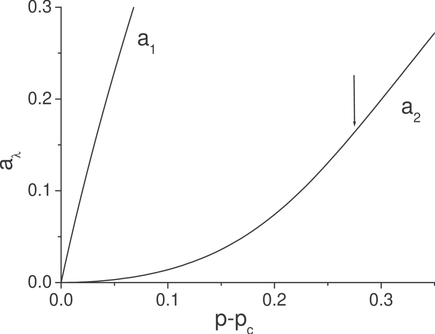
Figure 4: Amplitudes $a_{1}$ and $a_{2}$ of critical and transverse modes, respectively, versus $p-p_{c}$ in an assortative network with degree–degree distribution (44) and the same parameters as for the dotted curve in Fig. 3: $f(q_{1})=f(q_{2})=0$. The percolation threshold is $p_{c}=1/\lambda_{1}$. The arrow shows the point $p=1/\lambda_{2}$.

Model (44) has a modular structure. Modules are formed by vertices with equal degrees $q$. The number of modules is equal to the number of different degrees, $N_{d}$. In the limit $f(q)\rightarrow\infty$ for all $q$, this network consists of disconnected modules. Each module is a $q$-regular random graph. In this limit, the Pearson coefficient $r=1$, which corresponds to a perfectly assortative network Newman:n02 . If $f(q)$ is large but finite we get a weakly connected modules.

Equations (47) and (48) show that the largest eigenvalue $\lambda_{1}$ is larger than $\max\Lambda(q)$. All other eigenvalues lie in the range: $\min\Lambda(q)<\lambda<\max\Lambda(q)$. For example, if the function $\Lambda(q)$ is a monotonously increasing function, then there is only one eigenvalue in every interval $(\Lambda(q_{i}),\Lambda(q_{i+1}))$. If $\max\Lambda(q)<\infty$, then $\lambda_{2}$ is finite because $\lambda_{2}<\max\Lambda(q)$. $\lambda_{1}$ is finite at $\langle q^{2}\rangle<\infty$ and diverges at $\langle q^{2}\rangle\rightarrow\infty$. Equation (48) shows that the maximal eigenvector satisfies Eq. (30). Thus conditions I–III in Sec. IV are fulfilled if $\max\Lambda(q)$ is finite. In this case model (44) belongs to the same universality class as an uncorrelated random complex network with the identical $P(q)$, e.i., degree–degree correlations does not affect the critical behavior.

In Fig. 2 we present the results of numerical calculation of the largest and the second largest eigenvalues of the branching matrix for a scale-free degree distribution, $P(q)=Aq^{-4}$, and uniform assortative mixing $f(q)=f>0$. One can see that $\lambda_{1}$ and $\lambda_{2}$ are finite even correlations are strong, $f(q)=f\gg 1$.

In order to check our predictions, Eqs. (27) and (28), for the amplitudes of critical and transverse modes at the percolation threshold, we solved numerically Eq. (10) for model Eq. (44). We considered a simple network consisting of two groups of vertices with degrees $q_{1}=4$ and $q_{2}=11$ and the following degree distribution: $P(q_{1})=0.6$, $P(q_{2})=0.4$. In this situation the branching matrix has only two modes—a critical mode and a transverse one. The resulting dependence of the size $S$ of a giant connected component on $p$ is shown in Fig. 3. A giant connected component emerges at $p_{c}=1/\lambda_{1}$. One can also see a non-monotonous behavior of $dS(p)/dp$ which takes place when the occupation probability $p$ crosses $1/\lambda_{2}$. Figure 4 shows that the amplitudes of the critical and transverse modes near the percolation point behave in agreement with Eqs. (27) and (28), i.e., $a_{1}\propto(p-p_{c})$ and $a_{2}\propto(p-p_{c})^{2}$.

VI Critical behavior of strongly assortative networks

Let us consider the case when the function $\Lambda(q)$ is unbounded, i.e., $\max\Lambda(q)=\infty$. Then the sequence of eigenvalues $\lambda_{i}$ also is unbounded. In particular, both $\lambda_{1}$ and $\lambda_{2}$ are infinite. The condition II is not fulfilled. For example, we can choose the function $\Lambda(q)=\Lambda_{0}q^{-\alpha}$. It is unbound at $-1\leq\alpha<0$ and bounded at $\alpha\geq 0$. In the latter case, model (44) has the same critical behavior as an uncorrelated network with the identical degree distribution. In Fig. 5 this region of parameters $\alpha$ and the degree distribution exponent $\gamma$ is defined as region I.

In order to study percolation in model (44) for $-1\leq\alpha<0$, we rewrite Eq. (10) in the following form:

$$y_{q}=\frac{p\Lambda(q)}{q-1}\Bigl{[}1-\Bigl{(}1-y_{q}\Bigr{)}^{q-1}\Bigr{]}+\frac{z_{1}\rho(q)v}{q},$$ (51)

where the parameter $v$ plays the role of an effective field:

$$\!\!\!\!\!\!v=p\sum_{q}\rho(q)P(q)\Bigl{[}1-\Bigl{(}1-y_{q}\Bigr{)}^{q-1}\Bigr{]}$$

$$=\sum_{q}\frac{qy_{q}}{z_{1}\rho(q)f(q)}\Big{/}\Bigl{[}1+\sum_{q}\frac{1}{f(q)}\Bigr{]}.$$ (52)

At $p\ll 1$ and $q_{cut}\gg 1$ these equations have an approximate solution

$$y_{q}=\frac{p\Lambda(q)}{q-1}+\frac{z_{1}\rho(q)v}{q},\,\,\,\text{at}\,\,\,q\gg q_{p},$$

$$\,\,\,\,\,\,\,\,=\frac{z_{1}\rho(q)v}{q[1-p\Lambda(q)]},\,\,\,\text{at}\,\,\,q\ll q_{p},$$ (53)

where a characteristic degree $q_{p}$ is determined from the equation $p\Lambda(q_{p})=1$ which gives

$$q_{p}=(\Lambda_{0}p)^{1/\alpha}\gg 1.$$ (54)

Within this solution we have $(q-1)y_{q}\gg 1$ at $q\gg q_{p}$, though $y_{q}\ll 1$. This enables us to use the approximation:

$$1-\Bigl{(}1-y_{q}\Bigr{)}^{q-1}\approx 1.$$ (55)

For the degree distribution $P(q)=Aq^{-\gamma}$ with $\gamma>3$, a self-consistent solution of Eq. (52) is

$$v\approx\frac{Ap}{z_{1}\rho(\gamma-2)q_{p}^{\gamma-2}}\propto p^{(2-\gamma+\alpha)/\alpha}.$$ (56)

The leading contribution to $v$ is given by a sum over degrees $q>q_{p}$. Substituting solution (53) into Eq. (11), we obtain the size of a giant connected component:

$$S\propto pv\propto p^{(2-\gamma+2\alpha)/\alpha}.$$ (57)

Interestingly, the main contribution to $S$ comes from degrees $q<q_{p}$.

Figure 5: Phase diagram in the plane $(\gamma,\alpha)$ of model (44). Here $\gamma$ is the degree distribution exponent, $P(q)\propto q^{-\gamma}$, and $\alpha$ is the exponent of the function $\Lambda(q)\propto q^{-\alpha}$. In region I the critical behavior of the model is the same as that for an uncorrelated network with the identical degree distribution. In region II the sequence of eigenvalues is unbounded, and this model demonstrates a new critical exponents, see Table 1. The boundary between regions I and II is defined by the equation $\alpha=\min(0,\gamma-3)$.

For a slowly increasing function $\Lambda(q)=\Lambda_{0}\ln q$ (which corresponds to $\alpha\rightarrow 0$), we have $q_{p}=\exp(1/(p\Lambda_{0})$. Then, at an arbitrary $\gamma>3$, we obtain from Eq. (56) the following results:

$$v\propto pe^{-(\gamma-2)/(p\Lambda_{0})},$$ (58)

$$S\propto pv\propto p^{2}e^{-(\gamma-2)/(p\Lambda_{0})}.$$ (59)

On the other hand, for $2<\gamma<3$ we note that if $q_{cut}\rightarrow\infty$, then the series Eq. (52) is a singular function of $v$. Then, Eq. (52) takes the form:

$$v\approx apv^{\gamma-2}+\frac{Ap}{z_{1}\rho(\gamma-2)q_{p}^{\gamma-2}},$$ (60)

where $a=O(1)$ is a model dependent parameter. Here the first singular term is given by the sum over $q<q_{p}$ under the condition that $q_{p}v\ll 1$. The second term is given by degrees $q>q_{p}$. At $\gamma>3+\alpha$ we arrive at the solution Eq. (56) while at $2<\gamma<3+\alpha$ we obtain

$$v\propto p^{\beta}$$ (61)

with $\beta=1/(3-\gamma)$. The size of a giant connected component is $S\propto pv\propto p^{1+\beta}$. This is exactly the behavior that was found for an uncorrelated scale-free network for $2<\gamma<3$ cah02 ; cha03 . It means that degree-degree correlations are irrelevant at $2<\gamma<3+\alpha$.

Our results are summed up in Fig. 5 and Table 1. In region I, degree–degree correlations are irrelevant. They become relevant and lead to new critical exponents in the region of parameters $\gamma>3+\alpha$ and $-1<\alpha<0$ (region II in Fig. 5) where model (44) has an unbounded sequence of eigenvalues of the branching matrix.

VII Critical behavior of strongly disassortative networks

Vázquez and Moreno Vazquez:vm03 introduced networks with the following degree-degree distribution:

$$P(q^{\prime},q)=\frac{1}{z_{1}}(1-g_{q^{\prime}})q^{\prime}P(q^{\prime})(1-\delta_{q^{\prime},1})\delta_{q,1}$$

$$+\frac{1}{z_{1}}(1-g_{q})qP(q)(1-\delta_{q,1})\delta_{q^{\prime},1}$$

$$+\frac{1}{z_{1}^{2}G}g_{q^{\prime}}q^{\prime}P(q^{\prime})g_{q}qP(q)(1-\delta_{q^{\prime},1})(1-\delta_{q,1}),$$ (62)

where $G\equiv\sum_{q>1}g_{q}qP(q)/z_{1}$. The fraction of vertices of degree 1 is fixed by the following condition: $P(q=1)=\sum_{q>1}(1-g_{q})qP(q)/z_{1}$. In this model, a vertex of degree $q>1$ is connected to a vertex of a degree $q^{\prime}=1$ with probability $1-g_{q}$, and this vertex ($q>1$) is connected to a vertex of degree $q^{\prime}>1$ with probability $g_{q}g_{q}^{\prime}/G$. From Eq. (6) we obtain that the average nearest-neighbor’s degree of the vertices of degree $q$ is $B(q)\propto g_{q}$. These networks are disassortative for any monotonic decreasing function $g_{q}$.

One can show that the branching matrix has the largest eigenvalue

$$\lambda_{1}=\frac{1}{z_{1}G}\sum_{q>1}g_{q}^{2}q(q-1)P(q).$$ (63)

All other eigenvalues are zero, $\lambda_{i}=0$ for $i\geq 2$. Remarkably, this spectrum is similar to that of an uncorrelated network, see Eq. (16). The maximal eigenvector is

$$\Phi^{(1)}_{q}=n_{1}g_{q},$$ (64)

where $n_{1}$ is for normalization. Using this result, we find the local clustering coefficient $C(q)$, Eq. (90), of model (62):

$$C(q)=\frac{\lambda_{1}^{2}}{Nz_{1}^{2}G}q^{-2\alpha}.$$ (65)

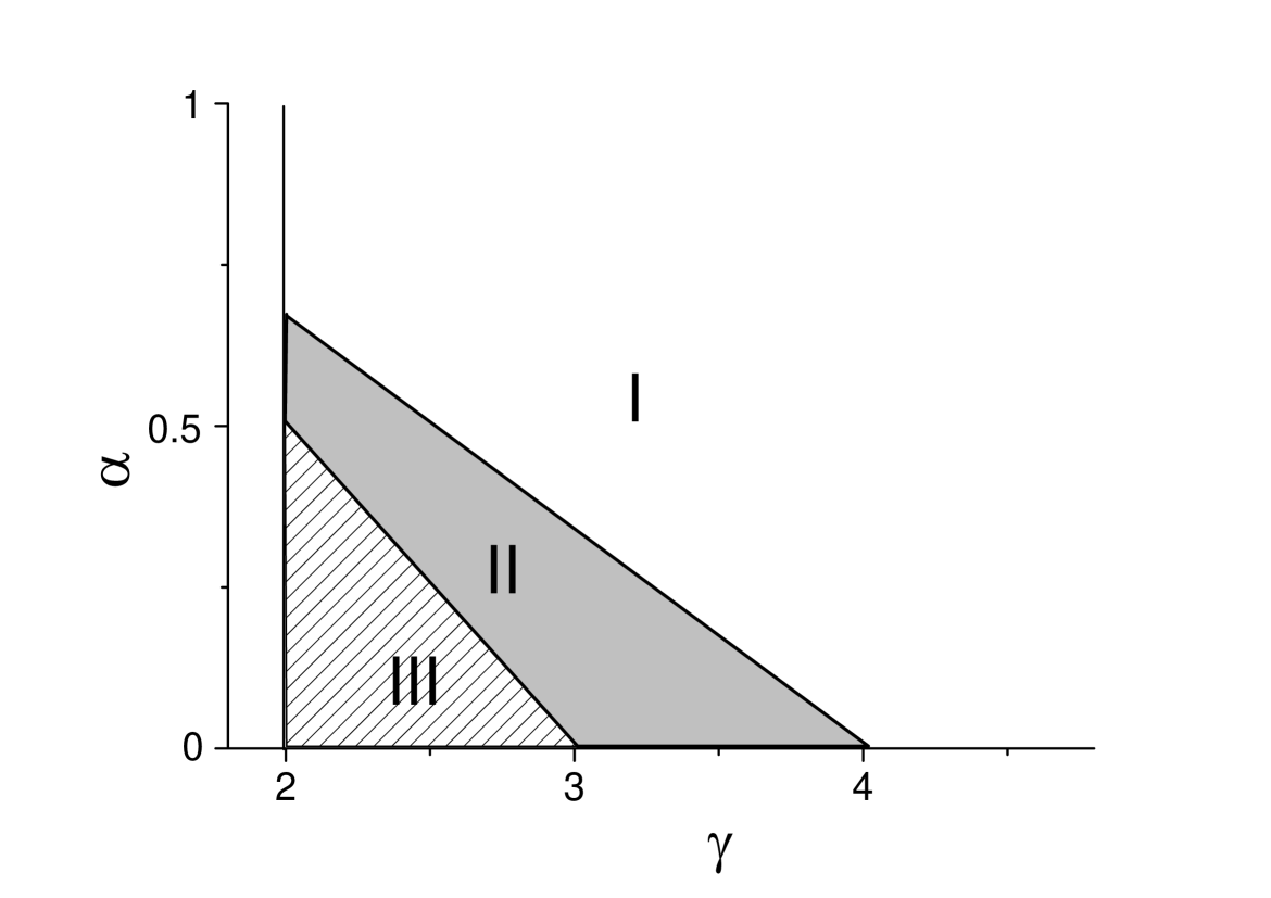
Figure 6: Phase diagram in the plane $(\gamma,\alpha)$ of model (62). Here $\gamma$ is the degree distribution exponent, $P(q)\propto q^{-\gamma}$, and $\alpha\geq 0$ is the exponent of the function $g(q)\propto q^{-\alpha}$. In region I this model shows the standard mean-field critical singularity with the critical exponent $\beta=1$. In regions II and III this model demonstrates a new critical behavior with the critical exponent depending on $\alpha$, see Table 1. The boundaries between regions I and II, and II and III, are defined by the equations $\alpha=(4-\gamma)/3$ and $\alpha=(3-\gamma)/2$, respectively.

Let us study the case of a scale-free degree distribution $P(q)\propto q^{-\gamma}$ and choose

$$g_{q}=q^{-\alpha}$$ (66)

with $\alpha\geq 0$. Zero exponent $\alpha=0$ corresponds to an uncorrelated network. If $\alpha>0$, then $\Phi^{(1)}_{q}\rightarrow 0$ at $q\rightarrow\infty$. It means that condition III in Sec. IV is not fulfilled.

The dependence of the percolation threshold $p_{c}$ on the parameters $\gamma$ and $\alpha$ was found in Vazquez:vm03 . Let us study the critical behavior of model (62). From Eq. (23) we find that the amplitudes $a_{i}=0$ for $i\geq 2$. Therefore, the order parameter is completely determined by the critical mode: $y_{q}=a_{1}\Phi^{(1)}_{q}$. The amplitude $a_{1}$ is determined by the following equation:

$$(p\lambda_{1}-1)a_{1}=p\lambda_{1}s_{1}(a_{1}),$$ (67)

where the function $s_{1}(x)$ is given by series Eq. (34). First we study the region of parameters $\alpha$ and $\gamma$, where

$$\alpha>\max(0,\frac{4-\gamma}{3}),\ \ \ \gamma>2$$ (68)

(region I in Fig. 6). Based on Eqs. (26) and (63) one can see that in this region, the coefficient $M_{111}$ and $\lambda_{1}$ are finite. Therefore, the percolation threshold is non-zero, $p_{c}=1/\lambda_{1}\neq 0$, e.i., this network is fragile against a random damage. The Eq. (67) has a solution $a_{1}\propto\tau^{\beta}$ with standard mean-field exponent $\beta=1$. Remarkably, if $\alpha>2/3$, then this standard critical behavior takes place at all $\gamma>2$. Region I includes a subregion with $2<\gamma<3$ where the second moment $\langle q^{2}\rangle$ of the degree distribution diverges. This is in contrast to an uncorrelated network with $2<\gamma<3$, which has $p_{c}=0$ and exponent $\beta=1/(3-\gamma)$.

Region II in Fig. 6 is defined by the inequalities

$$\frac{3-\gamma}{2}<\alpha<\frac{4-\gamma}{3},\ \ \ 2<\gamma<4.$$ (69)

In region II, $\lambda_{1}$ is finite while $M_{111}=\infty$. This points out that the function $s_{1}(x)$ is a singular function. The asymptotic behavior of this function is the following: $s_{1}(x)\propto x^{2-\nu}$ where $\nu=(4-3\alpha-\gamma)/(1-\alpha)>0$. Equation (67) gives $a_{1}\propto\tau^{\beta}$ with the exponent

$$\beta=\frac{1-\alpha}{\gamma-3+2\alpha}.$$ (70)

Region III in Fig. 6 is defined by the inequalities

$$0<\alpha<\frac{3-\gamma}{2},\,\,\,2<\gamma<3.$$ (71)

In this region both $\lambda_{1}$ and $M_{111}$ diverge. Therefore, $p_{c}=0$ and the network is robust against random damage. To find the order parameter we directly solve Eq. (10). The exact solution is $y_{q}=yg_{q}$ where $y$ satisfy

$$y=\frac{p}{z_{1}G}\sum_{q>1}g_{q}qP(q)\Bigl{[}1-(1-yg_{q})^{q-1}\Bigr{]}$$ (72)

The series in $y$ on the right-hand side has an asymptotic behavior $\propto y^{1-1/\beta}$, $y\ll 1$, where

$$\beta=\frac{1-\alpha}{3-2\alpha-\gamma}.$$ (73)

This leads to a solution $y\propto p^{\beta}$. The resulting size of a giant connected component is $S\propto py$.

Thus, strong disassortative correlations can dramatically change both the percolation threshold and the critical behavior. In a broad region of parameters $\gamma$ and $\alpha$, see Fig. 6 and Table 1, the critical properties of model (62) with disassortative mixing differ from those of a corresponding uncorrelated network.

VIII Conclusions

We have studied critical phenomena at the percolation transition in equilibrium complex networks with degree-degree correlations. Our consideration is based on the assumptions that a network is locally tree-like, i.e., clustering is negligibly small, and that only degree–degree correlations between the nearest neighboring vertices are present. The origin of degree–degree correlations is not relevant for our approach. These correlations can be intrinsic (i.e., they implicitly follow from other features of a network) or directly defined in a given network model.

We have demonstrated that both assortative and disassortative mixing affect not only the percolation threshold but can also change critical behavior at this percolation point. We have found necessary and sufficient conditions for a correlated network to have the same critical behavior as an uncorrelated network with the identical degree distribution. These conditions result from the fact that critical singularities at the percolation point are determined not only by a degree distribution, as for uncorrelated networks, but also spectral properties of the branching matrix. The resulting critical behavior of a correlated network belongs to the same universality class as percolation on an uncorrelated network if the following conditions are fulfilled: (I) the largest eigenvalue $\lambda_{1}$ of the branching matrix is finite if $\langle q^{2}\rangle$ is finite, or $\lambda_{1}\rightarrow\infty$ if $\langle q^{2}\rangle\rightarrow\infty$; (II) the second largest eigenvalues of the branching matrix is finite; (III) the sequence of entries of the eigenvector associated with the largest eigenvalue converges to a non-zero value. In this situation, one can say that degree–degree correlations (assortative or disassortative) are irrelevant for critical phenomena though they change the value of a percolation threshold. The critical exponents are completely determined by asymptotic behavior of degree distribution at large degrees.

Degree–degree correlations become relevant if at least one of these conditions is not fulfilled. We have proposed two simple models of correlated networks with strong assortative and disassortative mixing, where correlations dramatically change the critical behavior. As a result, the critical exponent becomes model dependent and hence non-universal. The advantage of these models is that they allow us, first, to change gradually from weak to strong mixing, and, second, to obtain the exact analytical solution of the percolation problem. In the assortative networks, proposed in this work, strong assortative mixing leads to an unbounded sequence of eigenvalues of the branching matrix, e.i., condition II is not fulfilled, which results in new critical singularities. Remarkably, in these networks the percolation threshold can be zero despite a finite second moment $\langle q^{2}\rangle$ of a degree distribution, in contrast to uncorrelated networks. (In uncorrelated networks, $p_{c}=0$ only if $\langle q^{2}\rangle\rightarrow\infty$.) We have also found an unusual critical behavior in a network with strong disassortative mixing where condition III is not fulfilled. Here the situation is just opposite to the strongly assortative network. Namely, in contrast to uncorrelated networks, the considered disassortative network can be fragile against random damage even if $\langle q^{2}\rangle\rightarrow\infty$. Moreover, we have shown that in a wide range of model parameters, strong disassortative mixing results in new critical singularities.

Many real-world networks and network models have non-zero clustering and long-range degree correlations. Intrinsic degree correlations are present, for example, in the static model of scale-free networks with degree exponent $2<\gamma<3$ lgkk06 and in some other models without self-loops and multiple connections. Unfortunately, these networks are clustered, and it is unknown whether their degree-degree correlations are short- or long-ranged. A generalization of the theory to networks with long-range degree correlations and non-zero clustering is a challenging problem Dorogovtsev:dgm07 .

We believe that our general conclusions concerning a strong influence of degree–degree correlations on critical singularities are true for various models of statistical physics defined on the top of correlated networks.

Appendix A Spectral properties of the branching matrix

Here we describe general properties of the eigenvalues $\lambda_{i}$ and eigenvectors $\Phi_{q}^{(i)}$ of the branching matrix (4). According to the Perron-Frobenius theorem, a real positive matrix $\widehat{B}$ has a positive real eigenvalue $\lambda_{1}$ such that $\lambda_{1}\geq|\lambda_{i}|$ for any eigenvalue $\lambda_{i}$ of $\widehat{B}$, see, e.g., Ref. Minc . Furthermore, there is an eigenvector with positive entries $\Phi_{q}^{(1)}>0$ corresponding to $\lambda_{1}$. $\lambda_{1}$ is the largest eigenvalue. The eigenvector associated with $\lambda_{1}$ is called a maximal eigenvector. If this matrix is positive then the largest eigenvalue is simple, i.e., non-generate.

One can show that a symmetric matrix

$$\widetilde{B}_{q,q^{\prime}}=\sqrt{\frac{\langle q\rangle(q-1)}{qP(q)}}P(q,q^{\prime})\sqrt{\frac{\langle q\rangle(q^{\prime}-1)}{q^{\prime}P(q^{\prime})}}$$ (74)

has the same eigenvalues $\lambda_{i}$ as the non-symmetric matrix $\widehat{B}$, i.e., $\sum_{q^{\prime}}\widetilde{B}_{qq^{\prime}}\widetilde{\Phi}_{q^{\prime}}^{(i)}=\lambda_{i}\widetilde{\Phi}_{q}^{(i)}$, where eigenvectors $\widetilde{\Phi}_{q}^{(i)}$ are related to the eigenvectors $\Phi_{q}^{(i)}$ as follows:

$$\widetilde{\Phi}_{q}^{(i)}=[q(q-1)P(q)/\langle q\rangle]^{1/2}\Phi_{q}^{(i)}.$$ (75)

This relationship between the non-symmetric matrix $\widehat{B}$ and the symmetric matrix $\widetilde{B}$ allows us to obtain the following spectral properties. First, since all eigenvalues of a symmetric real matrix are real, all eigenvalues $\lambda_{i}$ of $\widehat{B}$ are also real. They can be ordered as follows: $\lambda_{1}\geq\lambda_{2}\geq...\geq\lambda_{N_{d}}$. Second, the eigenvectors $\widetilde{\Phi}^{(i)}$ form a complete orthonormal basis set:

$$\sum_{q}\widetilde{\Phi}_{q}^{(i)}\widetilde{\Phi}_{q}^{(j)}=\delta_{i,j},$$ (76)

$$\sum_{\lambda}\widetilde{\Phi}_{q}^{(\lambda)}\widetilde{\Phi}_{q^{\prime}}^{(\lambda)}=\delta_{q,q^{\prime}}.$$ (77)

Using relation (75) we obtain Eqs. (14) and (15). Because the maximal eigenvalue $\lambda_{1}$ of the positive matrix $\widehat{B}$ is non-degenerate, this eigenvalue is strictly larger than the second largest eigenvalue $\lambda_{2}$. In other words, there is a gap between $\lambda_{1}$ and the second largest eigenvalue $\lambda_{2}$, $\lambda_{1}-\lambda_{2}>0$. A value of this gap is determined by a specific form of a joint degree–degree distribution $P(q^{\prime},q)$.

The largest eigenvalue $\lambda_{1}$ of a non-negative branching matrix $B_{qq^{\prime}}$ has the following upper boundary Minc :

$$\lambda_{1}\leq\max_{q}B(q).$$ (78)

Using the equation

$$\lambda_{1}=\max_{\Psi_{q}>0}\frac{\sum_{q,q^{\prime}}\Psi_{q^{\prime}}(q^{\prime}-1)P(q^{\prime},q)(q-1)\Psi_{q}}{\sum_{q}\Psi^{2}_{q}q(q-1)P(q)}$$ (79)

which directly follows from Eq. (13), we can find a lower boundary. Substituting $\Psi_{q}=1$, we get

$$\frac{1}{z_{2}}\sum_{q}B(q)q(q-1)P(q)\leq\lambda_{1}.$$ (80)

Unfortunately, no results are known for the second largest eigenvalue $\lambda_{2}$.

For an uncorrelated network, $P(q^{\prime},q)=q^{\prime}P(q^{\prime})qP(q)/\langle q\rangle^{2}$. In this case the matrix $\widehat{B}$ has the entries

$$B_{qq^{\prime}}=(q^{\prime}-1)q^{\prime}P(q^{\prime})/\langle q\rangle\equiv B_{qq^{\prime}}^{(0)}.$$ (81)

The largest eigenvalue of this matrix is

$$\lambda_{1}=z_{2}/z_{1}.$$ (82)

The normalized maximal eigenvector has equal entries

$$\Phi_{q}^{(1)}=[z_{1}/z_{2}]^{1/2}$$ (83)

for all $q$. There is also an ($N_{d}-1$)-degenerate zero eigenvalue, $\lambda_{2}=...=\lambda_{N_{d}}=0$. In this case the gap, $\lambda_{1}-\lambda_{2}$, in the spectrum is equal to $z_{2}/z_{1}$. Any vector $\Phi$ orthogonal to $\Phi^{(1)}$ in the sense of Eq. (3) is an eigenvector associated with this zero eigenvalue.

Let us consider a network in which a joint degree–degree distribution $P(q^{\prime},q)$ slightly deviates from $q^{\prime}P(q^{\prime})qP(q)/\langle q\rangle^{2}$, i.e.,

$$\max_{q}{\frac{|B(q)-\overline{B}|}{\overline{B}}}\ll 1,$$ (84)

where the branching coefficient $B(q)$ and the mean branching coefficient $\overline{B}$ are defined by Eqs. (6) and (8).

In order to find the largest eigenvalue, we write $\widehat{B}=\widehat{B}^{(0)}+\delta\widehat{B}$, where the matrix $\widehat{B}^{(0)}$ is given by Eq. (81), and $\delta\widehat{B}=\widehat{B}-\widehat{B}^{(0)}$ is a perturbation. In the first order of the perturbation theory we get:

$$\Phi_{q}^{(1)}\approx AB(q)/\overline{B},$$ (85)

$$\lambda_{1}\approx\frac{1}{z_{2}}\sum_{q}B(q)q(q-1)P(q).$$ (86)

Here A is a normalization constant. Equation (86) agrees with the lower boundary in Eq. (80). Let us analyze these results. First, the entries $\Phi_{q}^{(1)}$ of the maximal eigenvector are positive and lie in a bounded range. Second, we can rewrite the right-hand side of Eq. (86) as

$$\!\!\!\lambda_{1}\approx\overline{B}+\frac{1}{\overline{B}}\Biggl{[}\sum_{q,q^{\prime}}(q^{\prime}-1)P(q^{\prime},q)(q-1)-\overline{B}^{2}\Biggr{]}$$

$$=\overline{B}+r\sigma^{2}/\overline{B}.$$ (87)

We see that degree-degree correlations give a contribution which is proportional to the Pearson coefficient $r$, Eq. (9). Therefore, assortative mixing increases $\lambda_{1}$ while disassortative mixing decreases it. As a result we get inequality (20). With increasing degree–degree correlations the magnitude of the second largest eigenvalue $\lambda_{2}$ increases gradually from zero. Therefore, in a weakly correlated network the matrix $\widehat{B}$ has a finite gap $\lambda_{1}-\lambda_{2}>0$ which depends on a specific degree-degree distribution $P(q,q^{\prime})$.

Appendix B Relationship between the matrix $\widehat{B}$ and network parameters

Many structural parameters of correlated networks can be related with the spectrum of the branching matrix. The local clustering coefficient $C(q)$ of a vertex with degree $q$ is defined as follows: $C(q)\equiv t(q)/[q(q-1)/2]$, where $t(q)$ is the number of triangles (loops of length $3$) attached to this vertex, and $q(q-1)/2$ is the maximum possible number of such triangles. The clustering coefficient $C$ and the mean clustering $\overline{C}$ are given by the following equations:

$$C=\frac{1}{z_{2}}\sum_{q}(q-1)P(q)C(q),$$

$$\overline{C}=\sum_{q}P(q)C(q).$$ (88)

According to Ref. d04 , we can rewrite $C(q)$ in the following form:

$$C(q)=\frac{(\widehat{B}^{3})_{qq}}{Nq(q-1)P(q)}.$$ (89)

where $\widehat{B}$ is the branching matrix (4). Using this equation and Eq. (15), we find relationships between the clustering coefficients and the eigenvalues $\lambda_{i}$ and eigenvectors $\Phi_{q}^{(i)}$ of the branching matrix:

$$C(q)=\frac{1}{N\langle q\rangle}\sum_{i=1}\lambda_{i}^{3}(\Phi_{q}^{(i)})^{2},$$ (90)

$$C=\frac{1}{Nz_{2}}\sum_{i=1}\lambda_{i}^{3},$$ (91)

$$\overline{C}=\frac{1}{N\langle q\rangle}\sum_{i=1}\lambda_{i}^{3}\sum_{q}P(q)(\Phi_{q}^{(i)})^{2},$$ (92)

For an uncorrelated network, $C^{(un)}=z_{2}^{2}/(N\langle q\rangle^{3})$ n03 . In a network with assortative mixing the largest eigenvalue $\lambda_{1}$ is larger than $z_{2}/z_{1}$ according to Eq. (20). Therefore the clustering coefficient $C^{(as)}$ is larger than $C^{(un)}$. Similarly, in networks with disassortative mixing the clustering coefficient $C^{(dis)}$ is smaller then $C^{(un)}$. Thus we obtain an inequality:

$$C^{(dis)}<\frac{z_{2}^{2}}{N\langle q\rangle^{3}}<C^{(as)}.$$ (93)

Using Eq. (15), we obtain a useful relation between the average branching coefficient $B(q)$, Eq. (6), and the eigenvalues $\lambda_{i}$ and eigenfunctions $\Phi_{q}^{(i)}$:

$$B(q)=v_{1}\lambda_{1}\Phi_{q}^{(1)}+\sum_{i\geq 2}v_{i}\lambda_{i}\Phi_{q}^{(i)}$$ (94)

where $v_{i}=\sum_{q}w(q)\Phi_{q}^{(i)}$. This relation shows that the degree dependence of $B(q)$ is determined by the eigenvectors $\Phi_{q}^{(i)}$, mainly by the maximal eigenvector $\Phi_{q}^{(1)}$. Note that if $\lambda_{1}\to\infty$, then $B(q\to\infty)\to\infty$ but not vice versa.

The average number, $N_{l}(q^{\prime}|q)$, of vertices with degree $q^{\prime}$ at a distance $l$ from a vertex of degree $q$ can also be related with the branching matrix $\widehat{B}$:

$$N_{l}(q^{\prime}|q)=\frac{q(\widehat{B}^{l})_{qq^{\prime}}}{q^{\prime}-1}.$$ (95)

The mean intervertex distance $\overline{\ell}$ of the correlated network can be found from the equation:

$$N=1+\sum_{q^{\prime}}\sum_{n=1}^{\overline{\ell}}N_{l}(q^{\prime}|q)$$

$$=1+\langle q\rangle\sum_{\lambda}W(\lambda)\sum_{n=1}^{\overline{\ell}}\lambda^{n},$$ (96)

where

$$W(\lambda)=\frac{1}{\langle q\rangle^{2}}\Biggl{[}\sum_{q}qP(q)\Phi_{q}^{(\lambda)}\Biggr{]}\Biggl{[}\sum_{q}q(q-1)P(q)\Phi_{q}^{(\lambda)}\Biggr{]}.$$ (97)

In a network with a finite gap between the largest the second largest eigenvalues, $\lambda_{2}$, the leading contribution into the right-hand side is given by the terms with $\lambda_{1}$. As a result we obtain the following estimate of $\overline{\ell}$ for a correlated network:

$$\overline{\ell}\approx\frac{\ln N}{\ln\lambda_{1}}.$$ (98)

Note that an uncorrelated network has a mean intervertex distance $\overline{\ell}\approx\ln N/\ln(z_{2}/z_{1})$. Using (20) we find that for a given degree distribution $P(q)$ a network with assortative mixing has a smaller intervertex distance $\overline{\ell}^{(as)}$ than an uncorrelated network, while a network with disassortative mixing has a larger $\overline{\ell}^{(dis)}$:

$$\overline{\ell}^{(as)}<\frac{\ln N}{\ln(z_{2}/z_{1})}<\overline{\ell}^{(dis)}.$$ (99)

Appendix C Entropy of a correlated network with a modular structure

Here we describe a statistical ensemble of assortative networks with degree–degree correlations, Eq. (44). The probability $P_{a}(a_{ij})$ that an edge between vertices $i$ and $j$ of degrees $q_{i}$ and $q_{j}$ is present ($a_{ij}=1$) or absent ($a_{ij}=0$) is

$$\!\!\!\!\!\!\!\!\!\!P_{a}(a_{ij})=\frac{z_{1}\rho^{2}}{N}(1+f(q_{i})\delta_{q_{i},q_{j}})\delta(a_{ij}-1)$$

$$\!\!\!\!\!+\Bigl{[}1-\frac{z_{1}\rho^{2}}{N}(1+f(q_{i})\delta_{q_{i},q_{j}})\Bigr{]}\delta(a_{ij}).$$ (100)

Here $a_{ij}$ are the entries of the adjacency matrix, $\rho$ and $f(q)$ are parameters. For an uncorrelated network (the configuration model), we have $\rho=1$ and $f(q)=0$. A positive $f(q)$ results in assortative mixing. Let a sequence of degrees [and so a degree distribution $P(q)$] be given. Then the probability of realization of a graph with a given adjacency matrix $a_{ij}$ is the product of probabilities $P_{a}(a_{ij})$ over all pairs of vertices:

$${\cal P}(\{a_{ij}\})=\frac{1}{{\cal Z}}\prod_{i=1}^{N-1}\prod_{j=i+1}^{N}P_{a}(a_{ij})\prod_{i=1}^{N}\delta\Bigl{(}\sum_{j}a_{ij}-q_{i}\Bigr{)}.$$ (101)

The delta-functions fix degrees of the vertices. ${\cal Z}$ is a normalization factor:

$${\cal Z}=\exp\Bigl{[}N\sum_{q}P(q)\ln\Bigr{[}\frac{1}{q!}\Bigl{(}\frac{q\rho}{\rho(q)}\Bigr{)}^{q}\Bigr{]}-\frac{1}{2}Ng\Bigr{]}.$$ (102)

where $g=\langle q\rangle[1+\rho^{2}+\rho^{2}\sum_{q}P^{2}(q)f(q)]$. In fact, ${\cal Z}$ is the partition function of this network ensemble (compare with a partition function for other network ensembles in Ref. b07 ). The function $\rho(q)$ is given by Eq. (45). At a given $\langle q\rangle$, parameters $\rho$ and $f(q)$ are coupled. The condition of the maximum of the entropy $\ln{\cal Z}$ with respect to the parameter $\rho$ leads to Eq. (46).

The average of a physical quantity $A(\{a_{ij}\})$ over the network ensemble is given by

$$\left\langle A\right\rangle_{\text{en}}=\int A(\{a_{ij}\}){\cal P}(\{a_{ij}\})\prod_{i=1}^{N-1}\prod_{j=i+1}^{N}da_{ij}.$$ (103)

In particular, for a graph with a given adjacency matrix $a_{ij}$, the degree-degree distribution $P(q,q^{\prime})$ is given by an average over edges,

$$P(q,q^{\prime})=\frac{1}{Nz_{1}}\sum_{i,j}\delta_{q_{i},q}a_{ij}\delta_{q_{j},q^{\prime}}.$$ (104)

Averaging this function over the network ensemble, we get Eq. (44).

References

- (1) R. Albert and A.-L. Barabási, Rev. Mod. Phys. 74, 47 (2002).
- (2) S. N. Dorogovtsev and J. F. F. Mendes, Adv. Phys. 51, 1079 (2002); Evolution of Networks: From Biological Nets to the Internet and WWW (Oxford University Press, Oxford, 2003).
- (3) M. E. J. Newman, SIAM Review 45, 167 (2003).
- (4) S. Boccaletti, V. Latora, Y. Moreno, M. Chavez, and D.-U. Hwang, Phys. Rep. 424, 175 (2006).
- (5) R. Pastor-Satorras, A. Vázquez and A. Vespignani, Phys. Rev. Lett. 87, 258701 (2001).
- (6) A. Vázquez, R. Pastor-Satorras, and A. Vespignani, Phys. Rev. E 65, 066130 (2002).
- (7) S. Maslov, K. Sneppen, A. Zaliznyak, Physica A, 333, 529 (2004).
- (8) S. Maslov and K. Sneppen, Science 296, 910 (2002).
- (9) M. E. J. Newman, Phys. Rev. Lett. 89, 208701 (2002).
- (10) S. N. Dorogovtsev, A. V. Goltsev, and J. F. F. Mendes, Rev. Mod. Phys. 80, 1275 (2008); eprint arXiv.org:0705.0010.
- (11) G. R. Grimmett, Percolation (Springer-Verlag, New York, 1989).
- (12) D. Stauffer and A. Aharony, Introduction to Percolation Theory, 2nd ed., (Taylor & Francis, London, 2003).
- (13) B. Bollobás and O. Riordan, Percolation, (Cambridge University Press, Cambridge, 2006).
- (14) R. Cohen, D. ben-Avraham, and S. Havlin, Phys. Rev. E 66, 036113 (2002).
- (15) R. Cohen, S. Havlin, and D. ben-Avraham, in Handbook of Graphs and Networks, eds. S. Bornholdt and H. G. Schuster (Wiley-VCH GmbH & Co., Weinheim, 2003), p. 85.
- (16) A. Vázquez and Y. Moreno, Phys. Rev. E 67, 015101 (R) (2003).
- (17) M. Boguñá and R. Pastor-Satorras, Phys. Rev. E 66, 047104 (2002).
- (18) M. Boguñá, R. Pastor-Satorras, and A. Vespignani, Lect. Notes Phys. 625, 127 (2003).
- (19) D. S. Callaway, J. E. Hopcroft, J. M. Kleinberg, M. E. J. Newman, and S. H. Strogatz, Phys. Rev. E 64, 041902 (2001).
- (20) S. N. Dorogovtsev, J. F. F. Mendes, and A. N. Samukhin Phys. Rev. E 64, 066110 (2001).
- (21) P. L. Krapivsky and S. Redner, Comput. Networks 39, 261 (2002).
- (22) D. Lancaster, J. Phys. A 35, 1179 (2002).
- (23) J. Kim, P. L. Krapivsky, B. Kahng, and S. Redner, Phys. Rev. E 66, 055101 (R) (2002).
- (24) M. Bauer and D. Bernard, J. Stat. Phys. 111, 703 (2003).
- (25) C. Coulomb and M. Bauer, Eur. Phys. J. B 35, 377 (2003).
- (26) P. L. Krapivsky and S. Redner, Physica A 340, 714 (2004).
- (27) V. L. Berezinskii, Sov. Phys. JETP 32, 493 (1970).
- (28) J. M. Kosterlitz and D. J. Thouless, J. Phys. C 6, 1181 (1973).
- (29) P. L. Krapivsky and S. Redner, Phys. Rev. E 63, 066123 (2001).
- (30) A. Barrat and R. Pastor-Satorras, Phys. Rev. E 71, 036127 (2005).
- (31) J.-S. Lee, K.-I. Goh, B. Kahng, and D. Kim, Eur. Phys. J. B 49, 231 (2006).
- (32) K.-I. Goh, B. Kahng, and D. Kim, Phys. Rev. Lett. 87, 278701 (2001).
- (33) J. D. Noh, Phys. Rev. E 76, 026116 (2007).
- (34) D. S. Callaway, M. E. J. Newman, S. H. Strogatz and D. J. Watts, Phys. Rev. Lett. 85, 5468 (2000).
- (35) M. E. J. Newman, S.H. Strogatz, and D.J. Watts, Phys. Rev. E 64, 026118 (2001).
- (36) H. Minc, Nonnegative matrices (A Wiley-Interscience Publication, New York, 1988).
- (37) R. Albert, H. Jeong, and A.-L. Barabási, Nature 406, 378 (2000).
- (38) A. V. Goltsev, S. N. Dorogovtsev, and J. F. F. Mendes, Phys. Rev. E 67, 026123 (2003).
- (39) G. Bianconi, eprint arXiv:0708.0153; eprint arXiv:0802.2888.
- (40) S. N. Dorogovtsev, Phys. Rev. E 69, 027104 (2004).
- (41) M. E. J. Newman, in Handbook of Graphs and Networks, eds. S. Bornholdt and H. G. Schuster (Wiley-VCH GmbH & Co., Weinheim, 2003), p. 35.