Gaussian Belief Propagation Solver
for Systems of Linear Equations

Abstract

The canonical problem of solving a system of linear equations arises in numerous contexts in information theory, communication theory, and related fields. In this contribution, we develop a solution based upon Gaussian belief propagation (GaBP) that does not involve direct matrix inversion. The iterative nature of our approach allows for a distributed message-passing implementation of the solution algorithm. We also address some properties of the GaBP solver, including convergence, exactness, its max-product version and relation to classical solution methods. The application example of decorrelation in CDMA is used to demonstrate the faster convergence rate of the proposed solver in comparison to conventional linear-algebraic iterative solution methods.

I Problem Formulation and Introduction

Solving a system of linear equations ${\bf A}{\bf x}={\bf b}$ is one of the most fundamental problems in algebra, with countless applications in the mathematical sciences and engineering. Given the observation vector ${\bf b}\in\mathbb{R}^{n},n\in\mathbb{N}^{\ast}$, and the data matrix ${\bf A}\in\mathbb{R}^{n\times n}$, a unique solution, ${\bf x}={\bf x}^{\ast}\in\mathbb{R}^{n}$, exists if and only if the data matrix ${\bf A}$ is full rank. In this contribution we concentrate on the popular case where the data matrices, ${\bf A}$, are also symmetric (e.g. , as in correlation matrices). Thus, assuming a nonsingular symmetric matrix ${\bf A}$, the system of equations can be solved either directly or in an iterative manner. Direct matrix inversion methods, such as Gaussian elimination (LU factorization, [1]-Ch. 3) or band Cholesky factorization ([1]-Ch. 4), find the solution with a finite number of operations, typically, for a dense $n\times n$ matrix, on the order of $n^{3}$. The former is particularly effective for systems with unstructured dense data matrices, while the latter is typically used for structured dense systems.

Iterative methods [2] are inherently simpler, requiring only additions and multiplications, and have the further advantage that they can exploit the sparsity of the matrix ${\bf A}$ to reduce the computational complexity as well as the algorithmic storage requirements [3]. By comparison, for large, sparse and amorphous data matrices, the direct methods are impractical due to the need for excessive row reordering operations. The main drawback of the iterative approaches is that, under certain conditions, they converge only asymptotically to the exact solution ${\bf x}^{\ast}$ [2]. Thus, there is the risk that they may converge slowly, or not at all. In practice, however, it has been found that they often converge to the exact solution or a good approximation after a relatively small number of iterations.

A powerful and efficient iterative algorithm, belief propagation (BP) [4], also known as the sum-product algorithm, has been very successfully used to solve, either exactly or approximately, inference problems in probabilistic graphical models [5]. In this paper, we reformulate the general problem of solving a linear system of algebraic equations as a probabilistic inference problem on a suitably-defined graph. We believe that this is the first time that an explicit connection between these two ubiquitous problems has been established. As an important consequence, we demonstrate that Gaussian BP (GaBP) provides an efficient, distributed approach to solving a linear system that circumvents the potentially complex operation of direct matrix inversion.

We shall use the following notations. The operator $\{\cdot\}^{T}$ denotes a vector or matrix transpose, the matrix ${\bf I}_{n}$ is a $n\times n$ identity matrix, while the symbols $\{\cdot\}_{i}$ and $\{\cdot\}_{ij}$ denote entries of a vector and matrix, respectively.

II The GaBP Solver

II-A From Linear Algebra to Probabilistic Inference

We begin our derivation by defining an undirected graphical model (i.e. , a Markov random field), $\mathcal{G}$, corresponding to the linear system of equations. Specifically, let $\mathcal{G}=(\mathcal{X},\mathcal{E})$, where $\mathcal{X}$ is a set of nodes that are in one-to-one correspondence with the linear system’s variables ${\bf x}=\{x_{1},\ldots,x_{n}\}^{T}$, and where $\mathcal{E}$ is a set of undirected edges determined by the non-zero entries of the (symmetric) matrix ${\bf A}$. Using this graph, we can translate the problem of solving the linear system from the algebraic domain to the domain of probabilistic inference, as stated in the following theorem.

Proposition 1 (Solution and inference)

The computation of the solution vector ${\bf x}^{\ast}$ is identical to the inference of the vector of marginal means $\mathbf{\mu}=\{\mu_{1},\ldots,\mu_{n}\}$ over the graph $\mathcal{G}$ with the associated joint Gaussian probability density function $p({\bf x})\sim\mathcal{N}(\mu\triangleq{\bf A}^{-1}{\bf b},{\bf A}^{-1})$.

Proof:

Another way of solving the set of linear equations ${\bf A}{\bf x}-{\bf b}=\mathbf{0}$ is to represent it by using a quadratic form $q({\bf x})\triangleq{\bf x}^{T}{\bf A}{\bf x}/2-{\bf b}^{T}{\bf x}$. As the matrix ${\bf A}$ is symmetric, the derivative of the quadratic form w.r.t. the vector ${\bf x}$ is given by the vector $\partial q/\partial{\bf x}={\bf A}{\bf x}-{\bf b}$. Thus equating $\partial q/\partial{\bf x}=\mathbf{0}$ gives the stationary point ${\bf x}^{\ast}$, which is nothing but the desired solution to ${\bf A}{\bf x}={\bf b}$. Next, one can define the following joint Gaussian probability density function

$$p({\bf x})\triangleq\mathcal{Z}^{-1}\exp{\big{(}-q({\bf x})\big{)}}=\mathcal{Z}^{-1}\exp{(-{\bf x}^{T}{\bf A}{\bf x}/2+{\bf b}^{T}{\bf x})},$$ (1)

where $\mathcal{Z}$ is a distribution normalization factor. Denoting the vector $\mathbf{\mu}\triangleq{\bf A}^{-1}{\bf b}$, the Gaussian density function can be rewritten as

$$p({\bf x}) = \mathcal{Z}^{-1}\exp{(\mathbf{\mu}^{T}{\bf A}\mathbf{\mu}/2)}$$ (2)

$$\times \exp{(-{\bf x}^{T}{\bf A}{\bf x}/2+\mathbf{\mu}^{T}{\bf A}{\bf x}-\mathbf{\mu}^{T}{\bf A}\mathbf{\mu}/2)}$$

$$= \mathcal{\zeta}^{-1}\exp{\big{(}-({\bf x}-\mathbf{\mu})^{T}{\bf A}({\bf x}-\mathbf{\mu})/2\big{)}}$$

$$= \mathcal{N}(\mathbf{\mu},{\bf A}^{-1}),$$

where the new normalization factor $\mathcal{\zeta}\triangleq\mathcal{Z}\exp{(-\mathbf{\mu}^{T}{\bf A}\mathbf{\mu}/2)}$. It follows that the target solution ${\bf x}^{\ast}={\bf A}^{-1}{\bf b}$ is equal to $\mathbf{\mu}\triangleq{\bf A}^{-1}{\bf b}$, the mean vector of the distribution $p({\bf x})$, as defined above (1). Hence, in order to solve the system of linear equations we need to infer the marginal densities, which must also be Gaussian, $p(x_{i})\sim\mathcal{N}(\mu_{i}=\{{\bf A}^{-1}{\bf b}\}_{i},P_{i}^{-1}=\{{\bf A}^{-1}\}_{ii})$, where $\mu_{i}$ and $P_{i}$ are the marginal mean and inverse variance (sometimes called the precision), respectively. ∎

According to Proposition 1, solving a deterministic vector-matrix linear equation translates to solving an inference problem in the corresponding graph. The move to the probabilistic domain calls for the utilization of BP as an efficient inference engine.

II-B Belief Propagation in Graphical Model

Belief propagation (BP) is equivalent to applying Pearl’s local message-passing algorithm [4], originally derived for exact inference in trees, to a general graph even if it contains cycles (loops). BP has been found to have outstanding empirical success in many applications, e.g. , in decoding Turbo codes and low-density parity-check (LDPC) codes. The excellent performance of BP in these applications may be attributed to the sparsity of the graphs, which ensures that cycles in the graph are long, and inference may be performed as if the graph were a tree.

Given the data matrix ${\bf A}$ and the observation vector ${\bf b}$, one can write explicitly the Gaussian density function, $p({\bf x})$ (2), and its corresponding graph $\mathcal{G}$ consisting of edge potentials (‘compatibility functions’) $\psi_{ij}$ and self potentials (‘evidence’) $\phi_{i}$. These graph potentials are simply determined according to the following pairwise factorization of the Gaussian function (1)

$$p({\bf x})\propto\prod_{i=1}^{n}\phi_{i}(x_{i})\prod_{\{i,j\}}\psi_{ij}(x_{i},x_{j}),$$ (3)

resulting in $\psi_{ij}(x_{i},x_{j})\triangleq\exp(-x_{i}A_{ij}x_{j})$ and $\phi_{i}(x_{i})\triangleq\exp\big{(}b_{i}x_{i}-A_{ii}x_{i}^{2}/2\big{)}$. Note that by completing the square, one can observe that $\phi_{i}(x_{i})\propto\mathcal{N}(\mu_{ii}=b_{i}/A_{ii},P_{ii}^{-1}=A_{ii}^{-1})$. The graph topology is specified by the structure of the matrix ${\bf A}$, i.e. , the edges set $\{i,j\}$ includes all non-zero entries of ${\bf A}$ for which $i>j$.

The BP algorithm functions by passing real-valued messages across edges in the graph and consists of two computational rules, namely the ‘sum-product rule’ and the ‘product rule’. In contrast to typical applications of BP in coding theory [6], our graphical representation resembles a pairwise Markov random field[5] with a single type of propagating message, rather than a factor graph [7] with two different types of messages, originating from either the variable node or the factor node. Furthermore, in most graphical model representations used in the information theory literature the graph nodes are assigned discrete values, while in this contribution we deal with nodes corresponding to continuous variables. Thus, for a graph $\mathcal{G}$ composed of potentials $\psi_{ij}$ and $\phi_{i}$ as previously defined, the conventional sum-product rule becomes an integral-product rule [8] and the message $m_{ij}(x_{j})$, sent from node $i$ to node $j$ over their shared edge on the graph, is given by

$$m_{ij}(x_{j})\propto\int_{x_{i}}\psi_{ij}(x_{i},x_{j})\phi_{i}(x_{i})\prod_{k\in\textrm{N}(i)\setminus j}m_{ki}(x_{i})dx_{i}.$$ (4)

The marginals are computed (as usual) according to the product rule

$$p(x_{i})=\alpha\phi_{i}(x_{i})\prod_{k\in\textrm{N}(i)}m_{ki}(x_{i}),$$ (5)

where the scalar $\alpha$ is a normalization constant. The set of graph nodes $\textrm{N}(i)$ denotes the set of all the nodes neighboring the $i$th node. The set $\textrm{N}(i)\backslash j$ excludes the node $j$ from $\textrm{N}(i)$.

II-C The Gaussian BP Algorithm

Gaussian BP is a special case of continuous BP, where the underlying distribution is Gaussian. Now, we derive the Gaussian BP update rules by substituting Gaussian distributions into the continuous BP update equations (4)-(5). Before describing the inference algorithm performed over the graphical model, we make the elementary but very useful observation that the product of Gaussian densities over a common variable is, up to a constant factor, also a Gaussian density.

Lemma 2 (Product of Gaussians)

Let $f_{1}(x)$ and $f_{2}(x)$ be the probability density functions of a Gaussian random variable with two possible densities $\mathcal{N}(\mu_{1},P_{1}^{-1})$ and $\mathcal{N}(\mu_{2},P_{2}^{-1})$, respectively. Then their product, $f(x)=f_{1}(x)f_{2}(x)$ is, up to a constant factor, the probability density function of a Gaussian random variable with distribution $\mathcal{N}(\mu,P^{-1})$, where

$$P^{-1} = (P_{1}+P_{2})^{-1},$$ (6)

$$\mu = P^{-1}(P_{1}\mu_{1}+P_{2}\mu_{2}).$$ (7)

Proof:

The proof of this lemma is straightforward, thus omitted. ∎

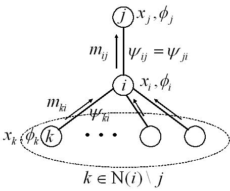
Figure 1: Graphical model: The neighborhood of node $i$.

Fig. 1. plots a portion of a certain graph, describing the neighborhood of node $i$. Each node (empty circle) is associated with a variable and self potential $\phi$, which is a function of this variable, while edges are identified with the pairwise (symmetric) potentials $\psi$. Messages propagate along the edges in both directions. The messages relevant for the computation of message $m_{ij}$ are shown in Fig. 1.). Looking at the right hand side of the integral-product rule (4), node $i$ needs to first calculate the product of all incoming messages, except for the message coming from node $j$. Recall that since $p({\bf x})$ is jointly Gaussian, the factorized self potentials $\phi_{i}(x_{i})\propto\mathcal{N}(\mu_{ii},P_{ii}^{-1})$ and similarly all messages $m_{ki}(x_{i})\propto\mathcal{N}(\mu_{ki},P_{ki}^{-1})$ are of Gaussian form as well.

As the terms in the product of the incoming messages and the self potential in the integral-product rule (4) are all a function of the same variable, $x_{i}$ (associated with the node $i$), then, according to the multivariate extension of Lemma 2, $\phi_{i}(x_{i})\prod_{k\in\textrm{N}(i)\backslash j}m_{ki}(x_{i})$ is proportional to a certain Gaussian distribution, $\mathcal{N}(\mu_{i\backslash j},P_{i\backslash j}^{-1})$. Applying the multivariate version of the product precision expression in (6), the update rule for the inverse variance is given by (over-braces denote the origin of each of the terms)

$$P_{i\backslash j}=\overbrace{P_{ii}}^{\phi_{i}(x_{i})}+\sum_{k\in\textrm{N}(i)\backslash j}\overbrace{P_{ki}}^{m_{ki}(x_{i})},$$ (8)

where $P_{ii}\triangleq A_{ii}$ is the inverse variance a-priori associated with node $i$, via the precision of $\phi_{i}(x_{i})$, and $P_{ki}$ are the inverse variances of the messages $m_{ki}(x_{i})$. Similarly, using (7) for the multivariate case, we can calculate the mean

$$\mu_{i\backslash j}=P_{i\backslash j}^{-1}\Big{(}\overbrace{P_{ii}\mu_{ii}}^{\phi_{i}(x_{i})}+\sum_{{k}\in\textrm{N}(i)\backslash j}\overbrace{P_{ki}\mu_{ki}}^{m_{ki}(x_{i})}\Big{)},$$ (9)

where $\mu_{ii}\triangleq b_{i}/A_{ii}$ is the mean of the self potential and $\mu_{ki}$ are the means of the incoming messages.

Next, we calculate the remaining terms of the message $m_{ij}(x_{j})$, including the integration over $x_{i}$. After some algebraic manipulation, using the Gaussian integral $\int_{-\infty}^{\infty}\exp{(-ax^{2}+bx)}dx=\sqrt{\pi/a}\exp{(b^{2}/4a)}$, we find that the messages $m_{ij}(x_{j})$ are proportional to a normal distribution with precision and mean

$$P_{ij}=-A_{ij}^{2}P_{i\backslash j}^{-1},$$ (10)

$$\mu_{ij}=-P_{ij}^{-1}A_{ij}\mu_{i\backslash j}.$$ (11)

These two scalars represent the messages propagated in the GaBP-based algorithm.

Finally, computing the product rule (5) is similar to the calculation of the previous product and the resulting mean (9) and precision (8), but including all incoming messages. The marginals are inferred by normalizing the result of this product. Thus, the marginals are found to be Gaussian probability density functions $\mathcal{N}(\mu_{i},P_{i}^{-1})$ with precision and mean

$$P_{i}=\overbrace{P_{ii}}^{\phi_{i}(x_{i})}+\sum_{k\in\textrm{N}(i)}\overbrace{P_{ki}}^{m_{ki}(x_{i})},$$ (12)

$$\mu_{i}=P_{i\backslash j}^{-1}\Big{(}\overbrace{P_{ii}\mu_{ii}}^{\phi_{i}(x_{i})}+\sum_{{k}\in\textrm{N}(i)}\overbrace{P_{ki}\mu_{ki}}^{m_{ki}(x_{i})}\Big{)},$$ (13)

respectively.

For a dense data matrix, the number of messages passed on the graph can be reduced from $\mathcal{O}(n^{2})$ (i.e. , twice the number of edges) down to $\mathcal{O}(n)$ messages per iteration round by using a similar construction to Bickson et al.  [9]: Instead of sending a unique message composed of the pair of $\mu_{ij}$ and $P_{ij}$ from node $i$ to node $j$, a node broadcasts aggregated sums to all its neighbors, and consequently each node can retrieve locally $P_{i\backslash j}$ (8) and $\mu_{i\backslash j}$ (9) from the aggregated sums

$$\tilde{P}_{i} = P_{ii}+\sum_{{k}\in\textrm{N}(i)}P_{ki},$$ (14)

$$\tilde{\mu}_{i} = \tilde{P}_{i}^{-1}(P_{ii}\mu_{ii}+\sum_{k\in\textrm{N}(i)}P_{ki}\mu_{ki})$$ (15)

by means of a subtraction

$$P_{i\backslash j} = \tilde{P}_{i}-P_{ji},$$ (16)

$$\mu_{i\backslash j} = \tilde{\mu}_{i}-P_{i\backslash j}^{-1}P_{ji}\mu_{ji}.$$ (17)

The following pseudo-code summarizes the GaBP solver algorithm.

Algorithm 1 (GaBP solver)

1.	Initialize:	$\checkmark$ Set the neighborhood $\textrm{N}(i)$ to include
		$\forall k\neq i\texttt{ such that }A_{ki}\neq 0$.
		$\checkmark$ Fix the scalars
		$\quad\quad P_{ii}=A_{ii}$ and $\mu_{ii}=b_{i}/A_{ii}$, $\forall i$.
		$\checkmark$ Set the initial $i\rightarrow\textrm{N}(i)$ broadcast messages
		$\tilde{P_{i}}=0$ and $\tilde{\mu}_{i}=0$.
		$\checkmark$ Set the initial $k\rightarrow i,k\in\textrm{N}(i)$ internal scalars
		$P_{ki}=0$ and $\mu_{ki}=0$.
		$\checkmark$ Set a convergence threshold $\epsilon$.
2.	Iterate:	$\checkmark$ Broadcast the aggregated sum messages
		$\quad\quad\tilde{P}_{i}=P_{ii}+\sum_{{k}\in\textrm{N}(i)}P_{ki}$,
		$\quad\quad\tilde{\mu}_{i}=\tilde{P_{i}}^{-1}(P_{ii}\mu_{ii}+\sum_{k\in\textrm{N}(i)}P_{ki}\mu_{ki})$, $\forall i$
		(under chosen scheduling).
		$\checkmark$ Compute the $i\rightarrow j,i\in\textrm{N}(j)$ internal scalars
		$\quad\quad P_{ij}=-A_{ij}^{2}/(\tilde{P}_{i}-P_{ji})$,
		$\quad\quad\mu_{ij}=(\tilde{P_{i}}\tilde{\mu_{i}}-P_{ji}\mu_{ji})/A_{ij}$.
3.	Check:	$\checkmark$ If the internal scalars $P_{ij}$ and $\mu_{ij}$ did not
		converge (w.r.t. $\epsilon$), return to Step 2.
		$\checkmark$ Else, continue to Step 4.
4.	Infer:	$\checkmark$ Compute the marginal means
		$\mu_{i}=\big{(}P_{ii}\mu_{ii}+\sum_{k\in\textrm{N}(i)}P_{ki}\mu_{ki}\big{)}/\big{(}P_{ii}+\sum_{{k}\in\textrm{N}(i)}P_{ki}\big{)}=\tilde{\mu}_{i}$, $\forall i$.
		$(\checkmark$ Optionally compute the marginal precisions
		$P_{i}=P_{ii}+\sum_{k\in\textrm{N}(i)}P_{ki}=\tilde{P}_{i}\quad)$
5.	Solve:	$\checkmark$ Find the solution
		$\quad\quad x_{i}^{\ast}=\mu_{i}$, $\forall i$.

II-D Max-Product Rule

A well-known alternative to the sum-product BP algorithm is the max-product (a.k.a. min-sum) algorithm [5]. In this variant of BP, a maximization operation is performed rather than marginalization, i.e. , variables are eliminated by taking maxima instead of sums. For trellis trees (e.g. , graphical representation of convolutional codes or ISI channels), the conventional sum-product BP algorithm boils down to performing the BCJR algorithm, resulting in the most probable symbol, while its max-product counterpart is equivalent to the Viterbi algorithm, thus inferring the most probable sequence of symbols [7].

In order to derive the max-product version of the proposed GaBP solver, the integral(sum)-product rule (4) is replaced by a new rule

$$m_{ij}(x_{j})\propto\operatorname*{arg\,max}_{x_{i}}\psi_{ij}(x_{i},x_{j})\phi_{i}(x_{i})\prod_{k\in\textrm{N}(i)\setminus j}m_{ki}(x_{i}).$$ (18)

Computing $m_{ij}(x_{j})$ according to this max-product rule, one gets (the exact derivation is omitted)

$$m_{ij}(x_{j})\propto\mathcal{N}(\mu_{ij}=-P_{ij}^{-1}A_{ij}\mu_{i\backslash j},P_{ij}^{-1}=-A_{ij}^{-2}P_{i\backslash j}),$$ (19)

which is identical to the messages derived for the sum-product case (10)-(11). Thus interestingly, as opposed to ordinary (discrete) BP, the following property of the GaBP solver emerges.

Corollary 3 (Max-product)

The max-product (18) and sum-product (4) versions of the GaBP solver are identical.

III Convergence and Exactness

In ordinary BP, convergence does not guarantee exactness of the inferred probabilities, unless the graph has no cycles. Luckily, this is not the case for the GaBP solver. Its underlying Gaussian nature yields a direct connection between convergence and exact inference. Moreover, in contrast to BP, the convergence of GaBP is not limited to acyclic or sparse graphs and can occur even for dense (fully-connected) graphs, adhering to certain rules that we now discuss. We can use results from the literature on probabilistic inference in graphical models [8, 10, 11] to determine the convergence and exactness properties of the GaBP solver. The following two theorems establish sufficient conditions under which GaBP is guaranteed to converge to the exact marginal means.

Theorem 4

[8, Claim 4] If the matrix ${\bf A}$ is strictly diagonally dominant (i.e. , $|A_{ii}|>\sum_{j\neq i}|A_{ij}|,\forall i$), then GaBP converges and the marginal means converge to the true means.

This sufficient condition was recently relaxed to include a wider group of matrices.

Theorem 5

[10, Proposition 2] If the spectral radius (i.e. , the maximum of the absolute values of the eigenvalues) $\rho$ of the matrix $|{\bf I}_{n}-{\bf A}|$ satisfies $\rho(|{\bf I}_{n}-{\bf A}|)<1$, then GaBP converges and the marginal means converge to the true means.

There are many examples of linear systems that violate these conditions for which the GaBP solver nevertheless converges to the exact solution. In particular, if the graph corresponding to the system is acyclic (i.e. , a tree), GaBP yields the exact marginal means (and even marginal variances), regardless of the value of the spectral radius [8].

IV Relation to Classical Solution Methods

It can be shown (see also Plarre and Kumar [12]) that the GaBP solver (Algorithm 1) for a system of linear equations represented by a tree graph is identical to the renowned direct method of Gaussian elimination (a.k.a. LU factorization, [1]). The interesting relation to classical iterative solution methods [2] is revealed via the following proposition.

Proposition 6 (Jacobi and GaBP solvers)

The GaBP solver (Algorithm 1)

1. with inverse variance messages arbitrarily set to zero, i.e. , $P_{ij}=0,i\in\textrm{N}(j),\forall{j}$;

2. incorporating the message received from node $j$ when computing the message to be sent from node $i$ to node $j$, i.e. , replacing $k\in\textrm{N}(i)\backslash j$ with $k\in\textrm{N}(i)$;

is identical to the Jacobi iterative method.

Proof:

Arbitrarily setting the precisions to zero, we get in correspondence to the above derivation,

$$P_{i\backslash j} = P_{ii}=A_{ii},$$ (20)

$$P_{ij}\mu_{ij} = -A_{ij}\mu_{i\backslash j},$$ (21)

$$\mu_{i} = A_{ii}^{-1}(b_{i}-\sum_{k\in\textrm{N}(i)}A_{ki}\mu_{k\backslash i}).$$ (22)

Note that the inverse relation between $P_{ij}$ and $P_{i\backslash j}$ (10) is no longer valid in this case. Now, we rewrite the mean $\mu_{i\backslash j}$ (9) without excluding the information from node $j$,

$$\mu_{i\backslash j}=A_{ii}^{-1}(b_{i}-\sum_{k\in\textrm{N}(i)}A_{ki}\mu_{k\backslash i}).$$ (23)

Note that $\mu_{i\backslash j}=\mu_{i}$, hence the inferred marginal mean $\mu_{i}$ (22) can be rewritten as

$$\mu_{i}=A_{ii}^{-1}(b_{i}-\sum_{k\neq i}A_{ki}\mu_{k}),$$ (24)

where the expression for all neighbors of node $i$ is replaced by the redundant, yet identical, expression $k\neq i$. This fixed-point iteration (24) is identical to the element-wise expression of the Jacobi method[2], concluding the proof. ∎

Now, the Gauss-Seidel (GS) method can be viewed as a ‘serial scheduling’ version of the Jacobi method; thus, based on Proposition 6, it can be derived also as an instance of the serial (message-passing) GaBP solver. Next, since successive over-relaxation (SOR) is nothing but a GS method averaged over two consecutive iterations, SOR can be obtained as a serial GaBP solver with ‘damping’ operation [13].

V Application Example: Linear Detection

We examine the implementation of a decorrelator linear detector in a CDMA system with spreading codes based upon Gold sequences of length $N=7$. Two system setups are simulated, corresponding to $n=3$ and $n=4$ users. The decorrelator detector, a member of the family of linear detectors, solves a system of linear equations, ${\bf A}{\bf x}={\bf b}$, where the matrix ${\bf A}$ is equal to the $n\times n$ correlation matrix ${\bf R}$, and the observation vector ${\bf b}$ is identical to the $n$-length CDMA channel output vector ${\bf y}$. Thus, the vector of decorrelator decisions is determined by taking the signum (for binary signaling) of the vector ${\bf A}^{-1}{\bf b}={\bf R}^{-1}{\bf y}$. Note that ${\bf R}_{n=3}$ and ${\bf R}_{n=4}$ in this case are not strictly diagonally dominant, but their spectral radii are less than unity, since $\rho(|{\bf I}_{3}-{\bf R}_{n=3}|)=0.9008<1$ and $\rho(|{\bf I}_{4}-{\bf R}_{n=4}|)=0.8747<1$, respectively. In all of the experiments, we assumed the (noisy) output sample was the all-ones vector.

Algorithm Iterations $t$ (${\bf R}_{n=3}$) Iterations $t$ (${\bf R}_{n=4}$) Jacobi 111 24 GS 26 26 Parallel GaBP 23 24 Optimal SOR 17 14 Serial GaBP 16 13 Jacobi+Steffensen 59 $-$ Parallel GaBP+Steffensen 13 13 Serial GaBP+Steffensen 9 7

TABLE I: Convergence rate.

Table I compares the proposed GaBP solver with standard iterative solution methods [2], previously employed for CDMA multiuser detection (MUD). Specifically, MUD algorithms based on the algorithms of Jacobi, GS and (optimally weighted) SOR were investigated [14, 15, 16]. Table I lists the convergence rates for the two Gold code-based CDMA settings. Convergence is identified and declared when the differences in all the iterated values are less than $10^{-6}$. We see that, in comparison with the previously proposed detectors based upon the Jacobi and GS algorithms, the serial (asynchronous) message-passing GaBP detector converges more rapidly for both $n=3$ and $n=4$ and achieves the best overall convergence rate, surpassing even the optimal SOR-based detector. Further speed-up of the GaBP solver can be achieved by adopting known acceleration techniques from linear algebra. Table I demonstrates the speed-up of the GaBP solver obtained by using such an acceleration method, termed Steffensen’s iterations [17], in comparison with the accelerated Jacobi algorithm (diverged for the 4 users setup). We remark that this is the first time such an acceleration method is examined within the framework of message-passing algorithms and that the region of convergence of the accelerated GaBP solver remains unchanged.

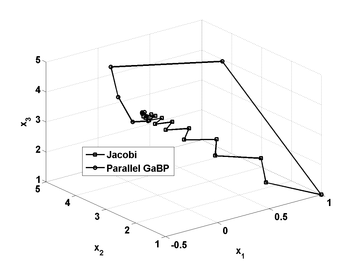
Figure 2: Convergence visualization.

The convergence contours for the Jacobi and parallel (synchronous) GaBP solvers for the case of 3 users are plotted in the space of $\{x_{1},x_{2},x_{3}\}$ in Fig. 2. As expected, the Jacobi algorithm converges in zigzags directly towards the fixed point. It is interesting to note that the GaBP solver’s convergence is in a spiral shape, hinting that despite the overall convergence improvement, performance improvement is not guaranteed in successive iteration rounds. Further results and elaborate discussion on the application of GaBP specifically to linear MUD may be found in recent contributions [18, 19].

References

- [1] G. H. Golub and C. F. V. Loan, Matrix Computation, 3rd ed. Baltimore, MD: The Johns Hopkins University Press, 1996.
- [2] O. Axelsson, Iterative Solution Methods. Cambridge, UK: Cambridge University Press, 1994.
- [3] Y. Saad, Iterative Methods for Sparse Linear Systems. PWS Publishing company, 1996.
- [4] J. Pearl, Probabilistic Reasoning in Intelligent Systems: Networks of Plausible Inference. San Francisco: Morgan Kaufmann, 1988.
- [5] M. I. Jordan, Ed., Learning in Graphical Models. Cambridge, MA: The MIT Press, 1999.
- [6] T. Richardson and R. Urbanke, Modern Coding Theory. Cambridge University Press, 2007.
- [7] F. Kschischang, B. Frey, and H. A. Loeliger, “Factor graphs and the sum-product algorithm,” IEEE Trans. Inform. Theory, vol. 47, pp. 498–519, Feb. 2001.
- [8] Y. Weiss and W. T. Freeman, “Correctness of belief propagation in Gaussian graphical models of arbitrary topology,” Neural Computation, vol. 13, no. 10, pp. 2173–2200, 2001.
- [9] D. Bickson, D. Dolev, and Y. Weiss, “Modified belief propagation for energy saving in wireless and sensor networks,” in Leibniz Center TR-2005-85, School of Computer Science and Engineering, The Hebrew University, 2005. [Online]. Available: http://leibniz.cs.huji.ac.il/tr/842.pdf
- [10] J. K. Johnson, D. M. Malioutov, and A. S. Willsky, “Walk-sum interpretation and analysis of Gaussian belief propagation,” in Advances in Neural Information Processing Systems 18, Y. Weiss, B. Schölkopf, and J. Platt, Eds. Cambridge, MA: MIT Press, 2006, pp. 579–586.
- [11] D. M. Malioutov, J. K. Johnson, and A. S. Willsky, “Walk-sums and belief propagation in Gaussian graphical models,” Journal of Machine Learning Research, vol. 7, Oct. 2006.
- [12] K. Plarre and P. Kumar, “Extended message passing algorithm for inference in loopy Gaussian graphical models,” Ad Hoc Networks, 2004.
- [13] K. M. Murphy, Y. Weiss, and M. I. Jordan, “Loopy belief propagation for approximate inference: An empirical study,” in Proc. of UAI, 1999.
- [14] A. Yener, R. D. Yates, and S. Ulukus, “CDMA multiuser detection: A nonlinear programming approach,” IEEE Trans. Commun., vol. 50, no. 6, pp. 1016–1024, June 2002.
- [15] A. Grant and C. Schlegel, “Iterative implementations for linear multiuser detectors,” IEEE Trans. Commun., vol. 49, no. 10, pp. 1824–1834, Oct. 2001.
- [16] P. H. Tan and L. K. Rasmussen, “Linear interference cancellation in CDMA based on iterative techniques for linear equation systems,” IEEE Trans. Commun., vol. 48, no. 12, pp. 2099–2108, Dec. 2000.
- [17] P. Henrici, Elements of Numerical Analysis. New York: John Wiley and Sons, 1964.
- [18] D. Bickson, O. Shental, P. H. Siegel, J. K. Wolf, and D. Dolev, “Linear detection via belief propagation,” in Proc. 45th Allerton Conf. on Communications, Control and Computing, Monticello, IL, USA, Sept. 2007.
- [19] ——, “Gaussian belief propagation based multiuser detection,” in IEEE Int. Symp. on Inform. Theory (ISIT), Toronto, Canada, July 2008.