OPED Reconstruction Algorithm for Limited Angle Problem

Abstract.

The structure of the reconstruction algorithm OPED permits a natural way to generate additional data, while still preserving the essential feature of the algorithm. This provides a method for image reconstruction for limited angel problems. In stead of completing the set of data, the set of discrete sine transforms of the data is completed. This is achieved by solving systems of linear equations that have, upon choosing appropriate parameters, positive definite coefficient matrices. Numerical examples are presented.

1. Introduction

Image reconstruction from x-ray data is the central problem of computed tomography (CT). An x-ray data is described by a line integral, called Radon transform, of the function that represents the image. A Radon transform of a function $f$ is denoted ${\mathcal{R}}f(\theta,t)$ where $\theta$ and $t$ are parameters in the line equation $\cos\theta x+\sin\theta y=t$. The image reconstruction means to recover the function from a set of line integrals by an approximation procedure, the reconstruction algorithm. For further background we refer to [5, 6, 13]. The quality of the reconstruction depends on how much x-ray data is available and the data geometry, meaning the distribution of the available x-ray lines, as well as on the algorithm being used. The ideal case is when the available data are exactly what the reconstruction algorithm need. Most of the algorithms, for example the FBP (filtered backprojection) algorithm, requires a full set of data that are well distributed in directions along a full circle of views. In many practical cases, however, x-rays in some of the directions could be missing. We then face the problem of reconstructing an image from a set of incomplete data, which is, however, intrinsically ill-posed. In order to apply an algorithm that requires a full set of data on the problem of incomplete data, one needs to derive approximations of the missing data from the available data, for example, by some type of interpolation process, which, however, has to be done carefully as the incomplete data is usually severely ill-posed.

In the present paper we consider the limited angle problem, a type of incomplete data problem for which the radon data ${\mathcal{R}}f(\theta,t)$ are given for $\theta$ in a subset of a half circle, and show that the reconstruction algorithm OPED (based on Orthogonal Polynomial Expansion on the Disk), studied recently in [19, 20, 21], permits a natural approximation for the missing data. The limited angle problem was studied extensively in [2, 8, 9, 10, 11, 15], see also [13]. The problem is known to be highly ill-posed ([2]). The approach in [8, 9, 10, 11] uses the singular value decomposition to generate the missing data, then uses FBP to reconstruct the image.

In our approach, we do not actually generate the missing Radon data per se, but what is missing for the OPED algorithm, which are the discrete sine transforms of the missing data. This algorithm for two dimensional images is based on orthogonal expansion on the disk; in fact, it is a discretization of the $N$-th partial sum of the Fourier expansion in orthogonal polynomials on the disk. One of the essential features of the algorithm is its preservation of polynomials of high degree. In other words, if the function that represents an image happens to be a polynomial of degree no more than $N$, then the algorithm reproduces the image exactly. For smooth functions, this ensures that OPED algorithm has a high order of convergence. In fact it is proved in [19] that it converges uniformly on the unit disk for functions that has second order continuous derivatives. Furthermore, numerical tests have shown that the algorithm reconstructs images accurately with high resolution for both phantom data and real data. Our main result in Section 3 shows that we can make use of the structure of the approximating function in OPED algorithm to generate what is missing for the algorithm, while still maintaining the feature of polynomial preserving, so that the algorithm can be used for the limited angle problem. The method completes the set of discrete sine transforms of the data by solving systems linear equations. We show how to choose parameters so that these matrices are positive definite. The ill-posedness of the limited angle problem is reflected in the ill-conditioning of the matrices. We discuss the dependence of the condition numbers on the parameters that appear in the algorithm, which serves as a guidance for the numerical experiments.

The paper is organized as follows. The follows section contains the background on OPED algorithm. In Section 3, we derive the algorithm for limited angle problem, provide a theoretic background, discuss conditions for the matrices to be positive definite, and study the conditional numbers of the matrices. The numerical results are reported and discussed in Section 4. A shot conclusion finishes the paper in Section 5.

2. Background and OPED algorithm

2.1. Background

Let $f(x,y)$ be a function defined on the unit disk $B=\{(x,y):x^{2}+y^{2}\leq 1\}$. A Radon transform of $f$ is a line integral,

$${\mathcal{R}}f(\theta,t):=\int_{I(\theta,t)}f(x,y)dxdy,\qquad 0\leq\theta\leq 2\pi,\quad-1\leq t\leq 1,$$

where $I(\theta,t)=\{(x,y):x\cos\theta+y\sin\theta=t\}\cap B$ is a line segment inside $B$. The central problem in CT is to recover the function $f(x,y)$, which represents an image, from its Radon transforms, which represent x-rays in mathematical terms. In reality, only a finite collection of x-ray data is available for reconstruction, which can be used to construct, in general, an approximation of $f$. An algorithm is a specific approximation process to $f$ based on the finite collection of data. There are many ways to construct the approximation process. The FBP algorithm is based on an interaction between Fourier and Radon transforms. OPED algorithm is based on orthogonal expansion on the disk.

Let $\Pi_{n}^{2}$ denote the space of polynomials of total degree at most $n$ in two variables. Let ${\mathcal{V}}_{n}(B)$ denote the space of orthogonal polynomials of degree $n$ on $B$ with respect to the Lebesgue measure. A function in $L^{2}(B)$ can be expanded in terms of orthogonal polynomials, that is,

(2.1) $$f(x)=\sum_{k=0}^{\infty}\operatorname{proj}_{k}f(x),\qquad\operatorname{proj}_{k}:L^{2}(B)\mapsto{\mathcal{V}}_{n}(B).$$

It turns out that the projection operator $\operatorname{proj}_{k}f$ has a natural connection to the Radon transforms. In fact, the following expression holds ([19], see also [7, 14, 1]),

(2.2) $$\operatorname{proj}_{k}f(x,y)=\frac{1}{N}\sum_{\nu=0}^{N-1}\frac{1}{\pi}\int_{-1}^{1}{\mathcal{R}}f(\phi_{\nu},t)U_{k}(t)dt(k+1)U_{k}(x\cos\phi_{\nu}+y\sin\phi_{\nu}),$$

where $\phi_{\nu}=\frac{2\pi\nu}{N}$ and $U_{k}(t)$ denotes the Chebyshev polynomial of the second kind,

(2.3) $$U_{k}(t)=\frac{\sin(k+1)\theta}{\sin\theta},\qquad t=\cos\theta.$$

The formula (2.2) allows us to construct a number of approximation processes based on the Radon data. Here are two that are of particular interests to us,

(2.4) $$S_{N}f(x):=\sum_{k=0}^{N-1}\operatorname{proj}_{k}f(x,y)\quad\hbox{and}\quad S_{N}^{\eta}f(x):=\sum_{k=0}^{N-1}\eta(\tfrac{k}{N})\operatorname{proj}_{k}f(x,y),$$

where $\eta$ is a smooth function in $C^{3}[0,\infty)$ such that $\eta(t)=1$ for $t\in[0,\tau]$, where $\tau$ is fixed with $0<\tau<1$, $\eta(t)=0$ for $t\geq 1$, and $\eta(t)$ is strictly decreasing on $[\tau,1]$. The function $S_{N}f$ is the best approximation to $f$ from $\Pi_{N}^{2}$ in $L^{2}(B)$ and it is a projection operator on $\Pi_{N}^{2}$, that is, $S_{N}f=f$ if $f\in\Pi_{N}^{2}$, while the function $S_{N}^{\eta}f$ approximates $f$ in uniform norm with the error of approximation in proportion to the best uniform approximation by polynomials of degree $\lfloor\tau N\rfloor$ and it satisfies $S_{N}^{\eta}f=f$ if $f\in\Pi_{\lfloor\tau N\rfloor}^{2}$ (see [18]). We can discretize $S_{N}f$ or $S_{N}^{\eta}f$, by applying a quadrature formula on the integral over $t$ in (2.2), to get an approximation to $f$ based on discrete Radon data, which is the essence of the OPED algorithm. If we choose Gaussian quadrature with respect to the Chebyshev weight, then the discretized approximation functions, denoted by $A_{N}f$ or $A_{N}^{\eta}f$, respectively, also preserve polynomials of appropriate degrees.

To be more precise, we work with the following explicit OPED algorithm.

Algorithm 2.1.

OPED Algorithm. Let $N_{d}$ and $N$ be two positive integers and $N_{d}\leq N$. Evaluate at each reconstruction points,

(2.5) $${\mathcal{A}}_{N}(x,y)=\frac{1}{N}\sum_{k=0}^{N_{d}-1}\sum_{\nu=0}^{N-1}\eta\left(\frac{k}{N_{d}}\right)\lambda_{k,\nu}(k+1)U_{k}(x\cos\phi_{\nu}+y\sin\phi_{\nu})$$

where $\phi_{\nu}=\frac{2\nu\pi}{N}$,

(2.6) $$\lambda_{k,\nu}=\frac{1}{N_{d}}\sum_{j=0}^{N_{d}-1}\sin(k+1)\psi_{j}{\mathcal{R}}({\phi_{\nu}},\cos\psi_{j}),\qquad\psi_{j}=\frac{(2j+1)\pi}{2N_{d}},$$

and $\eta(t)$ is a smooth function such that $\eta(t)=1$ on $[0,\tau]$ for a fixed $\tau$, $0<\tau<1$, and $\eta(t)\geq 0$ for $t\geq\tau$.

The image is reconstructed by the values of ${\mathcal{A}}_{N}(x,y)$ over a grid of reconstruction points. The function ${\mathcal{A}}_{N}(x,y)$ is a polynomial of degree $N_{d}$. As an operator, it preserves polynomials of degree $\lfloor\tau N_{d}\rfloor$, that is,

$${\mathcal{A}}_{N}f\equiv f\qquad\hbox{for all $f\in\Pi_{\lfloor\tau N_{d}\rfloor}^{2}$}.$$

Naturally $N_{d}$ and $N$ could be the same. For image reconstruction, we often take $N$ and $N_{d}$ as large as 1000, meaning that ${\mathcal{A}}_{N}f$ preserves polynomials of high degrees. The reconstruction has high quality, as supported by both theoretic study in [19] and by numerical experiments in [4, 20, 21]. A fast implementation of the algorithm is discussed in [20], which shows that we need ${\mathcal{O}}(N^{3})$ evaluations for reconstructing an image on a $M\times M$ grid, if $N_{d}\approx M\approx N$.

2.2. OPED algorithm with odd number of views

An x-ray enters an area in the angle $\phi$ is the same as the x-ray that exits with the angle $\pi+\phi$. For Radon transform, this is stated as

(2.7) $${\mathcal{R}}(\phi+\pi,t)={\mathcal{R}}(\phi,-t),\qquad 0\leq\phi\leq 2\pi.$$

As a result, we have been using the OPED algorithm with $N$ being an odd integer to avoid the repetition. For $N$ being odd, we can rewrite the formula of OPED algorithm so that the views are restricted to $[0,\pi]$ instead of $[0,2\pi]$. We state this as a proposition.

Proposition 2.2.

Let $N$ be an odd integer. Then we can replace $\phi_{\nu}=2\pi\nu/N$ in (2.5) and (2.6) by $\gamma_{\nu}=\pi\nu/N$.

Proof.

Let us define

$$\lambda_{k}(\phi)=\frac{1}{N_{d}}\sum_{j=0}^{N_{d}-1}\sin(k+1)\psi_{j}{\mathcal{R}}({\phi},\cos\psi_{j}).$$

Then $\lambda_{k,\nu}=\lambda_{k}(\phi_{\nu})$. Since $N$ is an odd integer, it follows readily that $\phi_{\nu}$ satisfies $\phi_{\nu+(N+1)/2}=\pi+\gamma_{2\nu+1}$. We also have that $\psi_{j}$ satisfies $\pi-\psi_{j}=\psi_{N_{d}-j-1}$. As a result, it follows from (2.7) that

$${\mathcal{R}}(\phi_{\nu+(N+1)/2},\cos\psi_{j})={\mathcal{R}}(\gamma_{2\nu+1},-\cos\psi_{j})={\mathcal{R}}(\gamma_{2\nu+1},\cos\psi_{N_{d}-j-1}).$$

Then, for $0\leq\nu\leq(N-3)/2$, we obtain

$$\lambda_{k}(\phi_{\nu+N/2}) =\frac{1}{N_{d}}\sum_{j=0}^{N_{d}-1}\sin(k+1)\psi_{j}{\mathcal{R}}(\gamma_{2\nu+1},\cos\psi_{N_{d}-j-1})$$

$$=\frac{1}{N_{d}}\sum_{j=0}^{N_{d}-1}\sin(k+1)\psi_{N_{d}-j-1}{\mathcal{R}}(\gamma_{2\nu+1},\cos\psi_{j})$$

$$=(-1)^{k}\frac{1}{N_{d}}\sum_{j=0}^{N_{d}-1}\sin(k+1)\psi_{j}{\mathcal{R}}(\gamma_{2\nu+1},\cos\psi_{j})=(-1)^{k}\lambda_{k}(\gamma_{2\nu+1}).$$

Let $\Omega_{k}(\phi):=\lambda_{k}(\phi)U_{k}(x\cos\phi+y\sin\phi)$. Using $\cos\phi_{\nu+\frac{N+1}{2}}=-\cos\gamma_{2\nu+1}$ and $\sin\phi_{\nu+\frac{N+1}{2}}=-\sin\gamma_{2\mu+1}$, as well as $U_{k}(-t)=(-1)^{k}U_{k}(t)$, it follows that

$$\Omega_{k}(\phi_{\nu+\frac{N+1}{2}})=(-1)^{k}\lambda_{k}(\gamma_{2\nu+1})U_{k}(-x\cos\gamma_{2\nu+1}-y\sin\gamma_{2\nu+1})=\Omega_{k}(\gamma_{2\nu+1}).$$

Consequently, we obtain

$$\sum_{\nu=0}^{N-1}\lambda_{k,\nu}U_{k}(x\cos\phi_{\nu}+y\sin\phi_{\nu})=\sum_{\nu=0}^{N-1}\Omega_{k}(\phi_{\nu})$$

$$\qquad=\sum_{\nu=0}^{\frac{N-1}{2}}\Omega_{k}(\gamma_{2\nu})+\sum_{\nu=0}^{\frac{N-3}{2}}\Omega_{k}(\gamma_{2\nu+1})=\sum_{\nu=0}^{N-1}\Omega_{k}(\gamma_{\mu}),$$

from which the proof of the stated result follows immediately. ∎

2.3. OPED algorithm with even number of views

If $N$ is even, the relation (2.7) shows that some of the rays coincide, so that the formulas in the OPED algorithm can be simplified somewhat. We summarize the essential part in the following proposition.

Proposition 2.3.

Let $N$ be an even integer. Then $\lambda_{k,\nu}$ defined in (2.6) satisfy

(2.8) $$\lambda_{k,\nu+N/2}=(-1)^{k}\lambda_{k,\nu},\qquad 0\leq\nu\leq N/2-1$$

and, furthermore,

(2.9) $$\sum_{\nu=0}^{N-1}\lambda_{k,\nu}U_{k}(x\cos\phi_{\nu}+y\sin\phi_{\nu})=2\sum_{\nu=0}^{N/2-1}\lambda_{k,\nu}U_{k}(x\cos\phi_{\nu}+y\sin\phi_{\nu}).$$

Proof.

Since $N$ is an even integer, $\phi_{\nu}$ satisfies $\phi_{\nu+N/2}=\pi+\phi_{\nu}$. We still have $\pi-\psi_{j}=\psi_{N_{d}-j-1}$. As a result, it follows from (2.7) that

$${\mathcal{R}}(\phi_{\nu+N/2},\cos\psi_{j})={\mathcal{R}}(\phi_{\nu},-\cos\psi_{j})={\mathcal{R}}(\phi_{\nu},\cos\psi_{N_{d}-j-1}).$$

Following the same line of the proof in the previous proposition, the above relation leads to (2.8) and (2.9) Following the same line of the proof in the previous proposition, the above relation leads to (2.8). Similarly, we have in this case $\Omega_{k}(\phi_{\nu+\frac{N}{2}})=\Omega_{k}(\phi_{\nu})$, from which (2.9) follows. ∎

As a of consequence of this proposition, the algorithm for even $N$ becomes:

Algorithm 2.4.

(OPED Algorithm for even $N$). Let $N$ be an even integer. Evaluate at each reconstruction points,

(2.10) $${\mathcal{A}}_{N}(x,y)=\frac{2}{N}\sum_{k=0}^{N_{d}-1}\sum_{\nu=0}^{N/2-1}\eta\left(\frac{k}{N_{d}}\right)\lambda_{k,\nu}(k+1)U_{k}(x\cos\phi_{\nu}+y\sin\phi_{\nu}),$$

where $\phi_{\nu}=\frac{2\pi\nu}{N}$ and $\lambda_{k,\nu}$ are given in (2.6).

In other words, we have (2.5) replaced by (2.10). Notice that the view angles in (2.10) are equally distributed over an half circle; that is, $\phi_{\nu}$ in (2.10) are in $[0,\pi]$. When we work with the limited angle problem, we will further assume that $N_{d}=N/2$ in (2.10); see Section 4.

For $N$ being even, a full data set for the OPED algorithm is then

(2.11) $${\mathcal{D}}_{N}:=\left\{g_{\nu,j}:={\mathcal{R}}(\phi_{\nu},\cos\psi_{j}):0\leq\nu\leq N/2-1,0\leq j\leq N-1\right\},$$

with angle $\phi_{\nu}$ distributed equally over a half circle (an arc of $180^{\circ}$).

3. Derivation of OPED algorithm for limited angle problem

In the limited angle problem, the data available consists of $g_{\nu,j}$ with $\phi_{\nu}$ distributed over an arc of less than $180^{\circ}$. We are particularly interested in the case that $N$ is even and the data is given by

(3.1) $${\mathcal{D}}_{r,N}:=\left\{g_{\nu,j}:r\leq\nu\leq N/2-1,\,0\leq j\leq N-1\right\},$$

where $r$ is a positive integer and $r<N/2-1$. In other words, the Radon projections correspond to the angles $\phi_{\nu_{0}},\ldots,\phi_{\nu_{r-1}}$ are missing from the data set ${\mathcal{D}}_{N}$. In this section we show how the structure of $A_{N}f$ can be explored to deal with such a problem.

3.1. Description of the idea

From the given data, we can compute (via FFT) every element in the set

(3.2) $$\Lambda_{r,N}:=\left\{\lambda_{k,\nu}:\,r\leq\nu\leq N/2-1,\,0\leq k\leq N_{d}-1\right\}.$$

To apply OPED algorithm, the missing data $\lambda_{k,\nu}$ for $0\leq k\leq N_{d}-1$ and $0\leq\nu\leq r-1$ are needed. We now describe our approach to complete the data set.

Note that the evaluation of ${\mathcal{A}}_{N}(x,y)$ in (2.10) can be carried out so long as we know all $\lambda_{k,\nu}$ for $0\leq\nu\leq N/2-1$ and $0\leq k\leq N_{d}-1$. The equation (2.10) is derived from (2.5) when $N$ is even. For more generality, we work in the following with (2.5) in which $N$ can be either even or odd, and accordingly with the available $\lambda_{k,\nu}$ given by

(3.3) $$\Lambda_{r,N}:=\left\{\lambda_{k,\nu}:\,r\leq\nu\leq N-1,\,0\leq k\leq N_{d}-1\right\}.$$

We will need a lemma on the Radon transform of orthogonal polynomials.

Lemma 3.1.

[12] If $P$ is an orthogonal polynomial in ${\mathcal{V}}_{k}(B)$, then for each $t\in(-1,1)$ and $0\leq\theta\leq 2\pi$,

$${\mathcal{R}}P(\theta,t)=\frac{2}{k+1}\sqrt{1-t^{2}}U_{k}(t)P(\cos\theta,\sin\theta).$$

Our new algorithm is based on following observation on $\lambda_{k,\nu}$ defined in (2.6).

Proposition 3.2.

If $f$ is a polynomial of degree at most $\tau N<N_{d}$, then $\lambda_{k,\nu}$ defined in (2.6) satisfies the system of equations

$$\lambda_{k,\mu}=\eta\left(\frac{k}{N_{d}}\right)\frac{1}{N}\sum_{\nu=0}^{N-1}\lambda_{k,\nu}U_{k}(\cos(\phi_{\mu}-\phi_{\nu})),$$

for $0\leq k\leq N_{d}-1$ and $0\leq\mu\leq N-1$.

Proof.

If $f$ is a polynomial of degree $\leq\tau N$, then ${\mathcal{A}}f=f$ and we have

(3.4) $$f(x,y)={\mathcal{A}}f(x,y)=\frac{1}{N}\sum_{k=0}^{N_{d}-1}\sum_{\nu=0}^{N-1}\lambda_{k,\nu}\eta\left(\frac{k}{N_{d}}\right)(k+1)U_{k}(x\cos\phi_{\nu}+y\sin\phi_{\nu}).$$

Since ${\mathcal{R}}f(\phi,t)/\sqrt{1-t^{2}}$ is a polynomial in $t$ of degree at most $\tau N$, as can be seen from Lemma 3.1, and we derived (2.5) by applying Gaussian quadrature of degree $2N_{d}-1$ with respect to the Chebyshev weight, it follows that

$$\lambda_{k,\mu}=\frac{1}{N_{d}}\sum_{j=0}^{N_{d}-1}\sin(k+1)\psi_{j}{\mathcal{R}}f(\phi_{\nu},\cos\psi_{j})=\frac{1}{\pi}\int_{-1}^{1}{\mathcal{R}}f(\phi_{\nu},t)U_{k}(t)dt.$$

It is known that $U_{k}(x\cos\phi_{\nu}+y\sin\phi_{\nu})$ is an orthogonal polynomial in ${\mathcal{V}}_{k}(B)$. Hence, applying Radon transform on (3.4) and using Lemma 3.1, we obtain that

$${\mathcal{R}}f(\phi,s)=\frac{2}{N}\sum_{\nu=0}^{N-1}\sum_{k=0}^{N_{d}-1}\eta\left(\frac{k}{N_{d}}\right)\lambda_{k,\nu}U_{k}(s)\sqrt{1-s^{2}}U_{k}(\cos(\phi-\phi_{\nu})).$$

Integrating against $U_{k}(s)ds$ and using the orthogonality of $U_{k}$, we end up with

$$\frac{1}{\pi}\int_{-1}^{1}{\mathcal{R}}f(\phi,s)U_{k}(s)ds=\eta\left(\frac{k}{N_{d}}\right)\frac{1}{N}\sum_{\nu=0}^{N-1}\lambda_{k,\nu}U_{k}(\cos(\phi-\phi_{\nu})).$$

Setting $\phi=\phi_{\mu}$ in the above relation proves the stated relation. ∎

Assuming that we are given the incomplete data (3.1). Then we can compute $\lambda_{k,\mu}$ in $\Lambda_{r,N}$ defined in (3.3). In order to apply the OPED algorithm, we do not need to know each individual missing data. It is sufficient to find the missing $\lambda_{k,\nu}$; that is, to find

$$\{\lambda_{k,\nu}:0\leq\nu\leq r-1,\,0\leq k\leq N_{d}-1\}.$$

The proposition suggests that we solve these $\lambda_{k,\nu}$ from the following linear system of equations: For $k=0,1,\ldots,N_{d}-1$, solve

(3.5) $$\lambda_{k,\mu}-\sum_{\nu=0}^{r-1}a_{\mu,\nu}^{(k)}\lambda_{k,\nu}=\sum_{\nu=r}^{N-1}a_{\mu,\nu}^{(k)}\lambda_{k,\nu},\qquad 0\leq\mu\leq r-1,$$

where for $k=0,1,\ldots,N_{d}-1$ and $0\leq\nu,\mu\leq N-1$, we define

$$a_{\mu,\nu}^{(k)}=\eta\left(\frac{k}{N_{d}}\right)\frac{\sin(k+1)(\phi_{\mu}-\phi_{\nu})}{N\sin(\phi_{\mu}-\phi_{\nu})},\quad\nu\neq\mu,\quad\hbox{and}\quad a_{\nu,\nu}^{(k)}=\eta\left(\frac{k}{N_{d}}\right)\frac{k+1}{N}.$$

Notice that $\lambda_{k,\nu}$ in the right hand side of (3.5) can be computed from the data in (3.1) by (2.6), so that they are known.

To summarize, the idea for the new algorithm is to solve (3.5) for the missing $\lambda_{k,\nu}$, and then apply OPED algorithm to the full set of $\lambda_{k,\nu}$ for reconstruction.

Solving (3.5) amounts to solve $N_{d}$ linear systems of equations of size $r\times r$. In order for this proposed method to work, it is necessary that the coefficient matrices of these systems are invertible, which we study in the following subsection.

3.2. Non-singularity of the matrices

In this section we assume $N_{d}=N$. We consider the case that $\eta(t)\equiv 1$ first and define

$$B_{k,r}^{(N)}:=\left[b_{\mu,\nu}^{k}\right]_{\mu,\nu\in{\mathcal{V}}_{r}},\quad b_{\mu,\nu}^{k}:=\frac{\sin(k+1)(\phi_{\mu}-\phi_{\nu})}{\sin(\phi_{\mu}-\phi_{\nu})}=U_{k}(\cos(\phi_{\mu}-\phi_{\nu}))$$

and

$$M_{k,r}^{(N)}:=I_{r}-N^{-1}B_{k,r}^{(N)}$$

for $0\leq k\leq N-1$ and $0\leq r\leq N-1$. The matrix $M_{k,r}^{(N)}$ is the coefficient matrix of (3.5) when $\eta(t)\equiv 1$. We note that these are symmetric matrices.

Theorem 3.3.

For $0\leq k,r\leq N-1$,
(a) the matrix $M_{k,r}^{(N)}$ is nonnegative definite with all eigenvalues in $[0,1]$;
(b) the matrix $M_{k,r}^{(N)}$ is positive definite if and only if $k+r<N$;
(c) If $k+r\geq N$, then zero is an eigenvalue of $M_{k,r}^{(N)}$ which has multiplicity equal to $k+r+1-N$.

Proof.

We start with an observation. Let $k=N-l-2$. Since $\phi_{\nu}=2\pi\nu/N$, it follows readily that $\sin(k+1)(\phi_{\mu}-\phi_{\nu})=-\sin(l+1)(\phi_{\mu}-\phi_{\nu})$. Hence, if $\mu\neq\nu$ then $b_{\mu,\nu}^{k}=-b_{\mu,\nu}^{l}$, whereas $b_{\nu,\nu}^{k}=k+1=N-(l+1)=N-b_{\nu,\nu}^{l}$. Consequently, we see that

(3.6) $$M_{N-l-2,r}^{(N)}=I_{r}-\frac{1}{N}\left[NI_{r}-B_{l,r}^{(N)}\right]=\frac{1}{N}B_{l,r}^{(N)}$$

for $0\leq N-l-2\leq N-1$ or $0\leq l\leq N-2$. Thus, we only need to consider $B_{k,r}^{(N)}$.

Let us define column vectors $\cos_{j}$ and $\sin_{j}$ by

$$\cos_{j}=(\cos j\phi_{\mu})_{\mu=0}^{r-1}\quad\hbox{and}\quad\sin_{j}=(\sin j\phi_{\mu})_{\mu=0}^{r-1},\quad j\geq 1,$$

and let $\mathbf{1}=(1,\ldots,1)$ also as a column vector. It is well known that $U_{n}(t)$ can be expressed as

$$U_{2m}(\cos\theta) \,=2\cos 2m\theta+2\cos(2m-2)\theta+\ldots+2\cos 2\theta+1$$

$$U_{2m+1}(\cos\theta) \,=2\cos(2m+1)\theta+2\cos(2m-1)\theta+\ldots+2\cos\theta.$$

Using the fact that $\cos j(\phi_{\mu}-\phi_{\nu})=\cos j\phi_{\mu}\cos j\phi_{\nu}+\sin j\phi_{\mu}\sin j\phi_{\nu}$, we can then write the matrix $B_{2m,r}^{(N)}$ as

$$B_{2m,r}^{(N)} =\mathbf{1}\cdot\mathbf{1}^{T}+\cos_{2}\cdot\cos_{2}^{T}+\sin_{2}\cdot\sin_{2}^{T}+\ldots+\cos_{2m}\cdot\cos_{2m}^{T}+\sin_{2m}\cdot\sin_{2m}^{T}$$

$$=X_{2m}X_{2m}^{T},$$

where $X_{2m}:=(\mathbf{1},\cos_{2},\sin_{2},\ldots,\cos_{2m},\sin_{2m})$ denotes the matrix that has $\mathbf{1},\cos_{2},\allowbreak\sin_{2},\ldots,\cos_{2m},\sin_{2m}$ as its column vectors. In the case of $k=2m+1$, we have

$$B_{2m+1,r}^{(N)}=X_{2m+1}X_{2m+1}^{T},\qquad X_{2m+1}:=(\cos_{1},\sin_{1},\cos_{3},\ldots,\cos_{2m+1},\sin_{2m+1}).$$

Considering the quadratic form $c^{T}B_{k,r}^{(N)}c$, if necessary, this shows that the matrix $B_{k,r}^{(N)}$, hence $N^{-1}B_{k,r}^{(N)}=I_{r}-M_{k,r}^{(N)}$, is nonnegative definite. Consequently, we see that the eigenvalues of $M_{k,r}^{(N)}$ are all bounded by $1$. Furthermore, the matrix $X_{k}$ is of the size $r\times(k+1)$ so that its rank is at most $\min\{k+1,r\}$. Consequently, if $X_{2m}c=0$ for a vector $c\in{\mathbb{R}}^{2m+1}$, then the trigonometric function

$$T_{2m}(t):=c_{1}+c_{2}\cos 2t+c_{2}\sin 2t+\ldots+c_{2m}\cos 2mt+c_{2m+1}\sin 2mt$$

vanishes on the points $t=\phi_{\nu}$ for $0\leq\nu\leq r-1$. If $r\geq 2m+1=k+1$, then the trigonometric polynomial $T_{2m}$ of degree $k$ vanishes on at least $2m+1$ points, which implies that $T_{2m}(t)\equiv 0$, so that $c=0$. It is easy to see that the same also holds for $k=2m+1$. Consequently, the columns of $X_{k}$ are linearly independent if $r\geq k+1$. If $r<k+1$, then we consider the $r\times r$ matrix, $Y_{k}$, formed by the first $r$-th columns of $X_{k}$. Considering $Y_{k}c=0$ as above, we see that $Y_{k}$ has full rank. Consequently, $\operatorname{rank}(X_{k})\geq\operatorname{rank}(Y_{k})\geq r$. Thus, we have proved that $\operatorname{rank}(X_{k})=\min\{k+1,r\}$.

If $k+1\geq r$ then, for $c\in{\mathbb{R}}^{r}$, $c^{T}B_{k,r}^{(N)}c=(c^{T}X_{k})^{2}=0$ so that $c=0$ as $\operatorname{rank}(X_{k})=r$. This shows that $B_{k,r}^{(N)}$ is positive definite, hence invertible. Whereas if $k+1<r$, then the rank of $B_{k,r}^{(N)}$ satisfies

$$\operatorname{rank}(B_{k,r}^{(N)})\geq\operatorname{rank}(X_{k})+\operatorname{rank}(X_{k})-(k+1)=k+1,$$

which shows that $\operatorname{rank}(B_{k,r}^{(N)})=k+1$. Hence, $B_{k,r}^{(N)}$ is singular in this case. Consequently we have proved that $B_{k,r}^{(N)}$ is positive definite if and only if $k+1\geq r$. Hence, by 3.6, the matrix $M_{k,r}^{(N)}$ is invertible if and only if $N-k-2+1\geq r$, which is equivalent to $k+r+1\leq N$.

Furthermore, if $k+1<r$, then the kernel of the matrix $B_{k,r}^{(N)}$ has dimension $r-(k+1)$. It follows that zero is an $r-(k+1)$ fold eigenvalue of the matrix. Again by (3.6), this is equivalent to that 0 is a $k+r+1-N$ fold eigenvalue of $M_{k,r}^{(N)}$. ∎

Since we need to solve (3.5) for all $k=0,1,\ldots,N-1$, the above result shows that the method will not work with $\eta(t)=1$ for any $r\geq 1$. The role that $\eta$ plays then becomes essential.

Let us define by $A_{k,r}^{(N)}$ the coefficient matrix of the system (3.5),

$$A_{k,r}^{(N)}:=I_{r}-\left[a_{\mu,\nu}^{(k)}\right]_{\mu,\nu\in{\mathcal{V}}_{r}}=I_{r}-\eta\left(\frac{k}{N}\right)\left[\frac{\sin(k+1)(\phi_{\mu}-\phi_{\nu})}{N\sin(\phi_{\mu}-\phi_{\nu})}\right]_{\mu,\nu\in{\mathcal{V}}_{r}},$$

where $I_{r}$ is the identity matrix of $r\times r$. This is also a symmetric matrix.

Theorem 3.4.

For $0\leq k,r\leq N-1$,
(a) if $k+r<N$, then the matrix $A_{k,r}^{(N)}$ is positive definite with all eigenvalues in $(0,1]$;
(b) if $k+r\geq N$, then the matrix $A_{k,r}^{(N)}$ is positive definite if and only if $\tau<1-r/N$.

Proof.

Let us denote the eigenvalues of a matrix $A$ by $\mu_{j}(A)$. By the definition, it is easy to see that $\mu_{j}(I_{r}-A_{k,r}^{(N)})=\eta(\tfrac{k}{N})\mu_{j}(I_{r}-M_{k,r}^{(N)})$, which implies that

(3.7) $$\mu_{j}(A_{k,r}^{(N)})=1-\eta(\tfrac{k}{N})+\eta(\tfrac{k}{N})\mu_{j}(M_{k,r}^{(N)}).$$

If $k+r<N$, then $\mu_{j}(M_{k,r}^{(N)})>0$ for $k+r<N$ by the theorem, and (3.7) implies that

$$\mu_{j}(A_{k,r}^{(N)})\geq\eta(\tfrac{k}{N})\mu_{j}(M_{k,r}^{(N)})\geq\eta(1-\tfrac{r}{N})\mu_{j}(M_{k,r}^{(N)})>0$$

since $\eta$ is non-increasing. Thus, for $k+r<N$, the matrix $A_{k,r}^{(N)}$ is positive definite. If $k+r\geq N$, then $M_{k,r}^{(N)}$ is nonnegative definite and has zero as an eigenvalue of multiplicity $k+r+1-N$. By (3.7), $A_{k,r}^{(N)}$ has $1-\eta(\tfrac{k}{N})$ as an eigenvalue of multiplicity $k+r+1-N$, and $A_{k,r}^{(N)}$ is positive definite if and only if $1-\eta(\frac{k}{N})>0$. Since $k+r\geq N$, we have $k=N-r,N-r+1,\ldots,N-1$. The assumption $\tau<1-r/N$ implies then that $\frac{k}{N}>\tau$ for $k+r\geq N$and, consequently, $1-\eta(\frac{k}{N})>0$ as $\eta$ is strictly decreasing on $[\tau,1]$. On the other hand, if $\tau=1-r/N$, then $\eta(\frac{N-r}{N})=\eta(\tau)=1$, so that $A_{k,r}^{(N)}$ has at least one zero eigenvalue when $k\geq N-r$ and, hence, is singular. ∎

As a consequence of this theorem, the matrices $A_{k,r}^{(N)}$ are all positive definite, hence invertible, if $r<(1-\tau)N$, where $\tau$ is the cut-off point in $\eta$. Thus, the condition $r<(1-\tau)N$ becomes a necessary condition for the algorithm to work. The reason that it is not sufficient lies in the numerical analysis. Theoretically, this condition is sufficient for $A_{k,r}^{(N)}$ to be invertible, but these matrices can be severely ill-conditioned which render the algorithm useless. For a positive definite matrix, the conditional number can be defined as the ratio of its largest eigenvalue over its smallest eigenvalue; that is, if $A$ is a $r\times r$ positive definite matrix with eigenvalues $\mu_{0},\ldots,\mu_{r-1}$, then

$$\mathrm{cond}(A):=\max_{0\leq j\leq r-1}\mu_{j}/\min_{0\leq j\leq r-1}\mu_{j}.$$

By (3.7) and the proof of the last theorem, if $k+r\geq N$, then the smallest eigenvalue of $A_{k,r}^{(N)}$ is $1-\eta(1-r/N)$, which can be very small when $\tau$ is close to $1-r/N$, as $\eta$ is strictly decreasing on $[\tau,1]$. Thus, it is necessary to take $r$ away from $1-\tau/N$, or, in other words, choose $\tau\leq 1-r/N+\varepsilon$ for some $\varepsilon>0$, to prevent the matrices $A_{k,r}^{(N)}$ become too ill-conditioned. On the other hand, when $k<\tau N$, we have $A_{k,r}^{(N)}=M_{k,r}^{(N)}$ and the matrices $M_{k,r}^{(N)}$ can be severely ill-conditioned. Thus, we often have to choose $\tau$ fairly small.

The eigenvalues of a related matrix, $C_{\Phi}$, were studied by Slepian in [16], where

$$C_{\Phi}=\left(c_{\mu,\nu}\right)_{\mu,\nu=0}^{r-1},\qquad c_{\mu,\nu}=\frac{\sin 2(\mu-\nu)\Phi}{(\mu-\nu)\pi}.$$

When $0<\Phi<\pi/2$, the eigenvalues of $C_{\Phi}$ are all between $(0,1)$ and the asymptotic of the largest eigenvalue $\mu_{0}$ is given in [16], which shows that $1-\mu_{0}$ can be exponentially decay as $r\to\infty$ (for precise statement, see [16, p. 1387] with the notation $\lambda_{k}(r,\Phi)$). If $\Phi=(k+1)\pi/N$, then we see that

$$c_{\mu,\nu}=\frac{k+1}{N}\frac{\sin(k+1)(\phi_{\mu}-\phi_{\nu})}{\phi_{\mu}-\phi_{\nu}},$$

which is similar to our $b_{\mu,\nu}^{k}$. For fixed $r,k$ and $N$ sufficiently large, the matrix $C_{\Phi}$ with $\Phi=(k+1)/N$ can be regarded as a close approximation to $B_{k,r}^{(N)}$, so that the eigenvalues of $C_{\Phi}$ gives some indication to the eigenvalues of $B_{k,r}^{(N)}$, and hence, those of $M_{k,r}^{(N)}$. However, a small perturbation in the entries of the matrix may lead to a large change in the eigenvalues; thus, it is of interesting to understand the eigenvalues of $M_{k,r}^{(N)}$ itself.

It should be mentioned that the matrix $C_{\Phi}$ and its eigenvalues are instrumental in deriving the singular values of the Radon transform ([8, 9]) as well as in completing data using singular value decomposition for the limited angle problem.

3.3. Algorithms for limited angle problem

We now consider the limited angle problem for which the given data set is (3.1) and we assume that $N$ is even. With simple modification, the method will work with odd $N$ as well.

Recall that for $N$ being even, we use (2.10) instead of (2.5), so that we replace $N$ in the systems of linear equations in (3.5) by $N/2$ and the coefficient matrices of these systems are non-singluar, according to Theorem 3.4, if $\tau<1-2r/N$ provided $N_{d}=N/2$. Below we sum up the algorithm for limited angle problem and we assume $N_{d}=N/2$.

Algorithm 3.5.

(Algorithm for limited angle problem) Given Radon data $\{g_{\nu,k}:\,r\leq\mu\leq N/2-1,0\leq k\leq N/2-1\}$, where $N$ is an even integer.

Setp 1. For $\mu=r,\ldots,N/2-1$, compute for $k=0,1,\ldots,N/2$ by FFT

$$\lambda_{k,\mu}=\sum_{j=0}^{N/2-1}g_{j,\mu}\sin(k+1)\psi_{j},\quad\psi_{j}=\frac{(2j+1)\pi}{N}.$$

Step 2. For a given $r$ choose $\tau$ so that $\tau<1-{2r}/{N}$ and choose an $\eta$. For $k=0,1,\ldots,N/2-1$ solve linear system of equations

(3.8) $$\lambda_{k,\mu}-\sum_{\nu=0}^{r-1}a_{\mu-\nu}^{(k)}\lambda_{k,\nu}=\sum_{\nu=r}^{N/2-1}a_{\mu-\nu}^{(k)}\lambda_{k,\nu},\qquad 0\leq\mu\leq r-1,$$

for $\lambda_{\mu,k}$, $0\leq\mu\leq r-1$, where

$$a_{\mu}^{(k)}=2\eta\left(\frac{2k}{N}\right)\frac{\sin(k+1)(\phi_{\mu})}{N\sin\phi_{\mu}},\quad\mu\neq 0,\quad\hbox{and}\quad a_{0}^{(k)}=2\eta\left(\frac{2k}{N}\right)\frac{k+1}{N}.$$

Step 3. Augmenting $\lambda_{k,\nu}$ computed in Step 1 and Step 2 to obtain a full set

$$\Lambda_{N}:=\{\lambda_{k,\mu}:0\leq\nu\leq N/2-1,0\leq k\leq N/2-1\}$$

and applying OPED Algorithm 2.4 on $\Lambda_{N}$ to reconstruct the image.

The output of the second step of the algorithm gives approximation for the missing data $\lambda_{0,k},\ldots,\lambda_{r-1,k}$ for $k=0,1,\ldots,N/2-1$. Notice that the algorithm does not complete the data set itself, what it completes is the set of sine transform s$\lambda_{k,\mu}$ of the data.

We now turn to the problem of how to choose $\eta$. Let $h_{k}(t)$ be a polynomial of degree $2k+1$ such that $h_{k}(0)=1$, $h_{k}^{(j)}(0)=0$ for $1\leq j\leq k$, and $h_{k}^{(j)}(1)=0$ for $0\leq j\leq k$. Such a polynomial is given explicitly by

$$h_{k}(t)=(1-t)^{k+1}\sum_{j=0}^{k}\binom{k+j}{j}t^{j}.$$

For a fixed $k$ we then define $\eta(t)$ by

(3.9) $$\eta(t):=\begin{cases}1,&0\leq t\leq\tau,\\ h_{k}\left(\frac{t-\tau}{1-\tau}\right),&\tau\leq t\leq 1\\ 0,&t>1.\end{cases}$$

Then $\eta\in C^{k}({\mathbb{R}})$ and it satisfies the desired property. The function $\eta$ curtails the values of high degree $\operatorname{proj}_{k}f$ in the expansion (2.4). Note that $\eta$ does not have to be zero at $t=1$. In fact, we can choose $\eta$ so that it is smooth on $[0,1]$, $\eta(1)=1$ for $0\leq t\leq\tau$ and $\eta(t)$ decreasing to $\eta(1)=\beta\geq 0$ on $[\tau,1]$. For example, here is such a function in $C^{3}$,

$$h_{k,\beta}(t):=(\beta-1)(3t^{2}-2t^{3})+1,$$

which when used in (3.9) gives a function in $C^{3}$ so that $\eta(1)=\beta$.

Naturally then we face the problem of how to choose $\tau$ and $\beta$. As the discussion at the end of the previous subsection shows, we should choose $\tau$ reasonably small to avoid the ill-conditioning of the matrices. The condition $\tau<1-\frac{2r}{N}$, however, is only a necessary condition; we need, in practice, $\tau$ substantially smaller. There is, however, a balance, as the algorithm preserves polynomials up to degree $\tau N_{d}$. Small $\tau$ means lower degree of polynomial preservation and less accuracy in reconstruction. This is where $\beta$ comes into the picture. If $\beta$ is large, say $\beta=0.95$, then $\eta$ will decreasing slowly down from 1 to 0.95, and we will have almost polynomial preserving property. The experiments have shown that larger $\beta$ may lead to worse condition numbers of the matrices, but the increasing is not drastic. On the other hand, the condition numbers increases drastically as $\tau$ increases.

For a fixed $N$ we can compute the condition numbers of $A_{k,r}^{(N)}$ numerically. We give an example. Notice that when $r$ is fixed, the available data $\{g_{k,\nu}:r\leq\nu\leq N/2-1,0\leq k\leq N/2-1\}$ is over an arc of $\pi-2\pi r/N$ radiant or the missing data is over

$$\alpha:=2\pi r/N=(360r/N)^{\circ}.$$

In other words, the given data is limited with angles over an arc of $180-\alpha$ degree and the missing data is over $\alpha$ degree.

Let us take for example $N=502$, which means the full data consists of $251$ views of equally spaced angles over $[0,\pi]$ and $251$ rays per view. For the incomplete data, if $r=21$, then the available data is limited to an arc of $165^{\circ}$, a $15^{\circ}$ difference from the full data. If $r=42$, then the data is limited to an arc of $150^{\circ}$, a $30^{\circ}$ difference from the full data. In Table 1, the the maximum of the condition numbers for our matrices, rounded to nearest integers, are given for different values of $\tau$ and $\beta$ in the cases of $r=21$ and $r=42$.

Table 1. Maximum of condition numbers

r = 21					r= 42
	$\tau$	$\beta$	$\max$			$\tau$	$\beta$	$\max$
	0.0	0.5	44			0.0	0.5	135
	0.0	0.9	160			0.0	0.9	503
	0.1	0.5	293			0.1	0.5	60295
	0.1	0.9	716			0.1	0.9	68296
	0.2	0.5	48900			0.2	0.5	$3.66715\times 10^{10}$
	0.2	0.9	48928			0.2	0.9	$3.66715\times 10^{10}$

For example, in the case of $r=21$, $\tau=0.0$ and $\beta=0.9$, the maximum of the condition number is merely 160. The maximum is very large in the case of $r=42$ and $\tau=0.2$, showing that the matrix $A_{k,r}^{(N)}$ is severely ill-conditioned for some $k$ in this case. Furthermore, the maximum of the condition numbers appears to increase drastically as $r$ increases as well as $\tau$ increases. Another interesting fact is that the dependence on $\beta$ appears to be insignificant for larger $r$ and larger $\tau$. In the Figure 1, the distribution of the condition numbers in the case of $r=42$, $\tau=0$ and $\tau=0.2$ is plotted, which shows that not all matrices among $A_{k,r}^{(N)}$ become ill-conditioned.

  

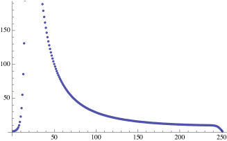
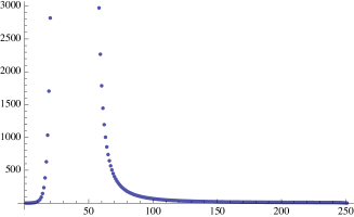
Figure 1. Condition numbers for $r=42$. Left: $\tau=0$. Right: $\tau=0.2$.

An interesting fact is that the conditional numbers in the case of $\tau=0$ remain reasonably in check even when $r$ is large, as seen in the following table, where we choose $\beta=0.9$ to compensate $\tau=0$.

Table 2. Maximum of condition numbers for $\tau=0$ and $\beta=0.9$

$r$	21	42	63	83	126
$\max$	160	503	1037	1757	4084
limited angle	$165^{\circ}$	$150^{\circ}$	$135^{\circ}$	$120^{\circ}$	$90^{\circ}$

In the case of $r=126$, the given data is distributed over an arc of $90^{\circ}$, which means that half of the full data. In this case, the maximum of the condition number is 4084 for $\beta=0.9$, which is still not too large. However, $\tau=0$ means that the algorithm no longer preserves polynomials and this is the case that should be avoided. Still, by choosing $\beta$ large so that the result of the sampling on the coefficients is not too far away from polynomial preservation, the case $\tau=0$ can be used to reconstruct of images as our numerical tests have shwon. In general, however, we should work with positive $\tau$ whenever we can. This is supported by the numerical experiments discussed in the next section.

4. Numerical Experiments and Discussions

We have applied the algorithm in the previous section on several examples, which are presented and discussed below. Recall that our data of limited angle consists of $\{g_{\nu,k}:r\leq\nu\leq N/2-1,0\leq k\leq N/2-1\},$where $N$ is an even integer, and the angle within which the data is distributed is, for a given $r$, $180^{\circ}-(360r/N)^{\circ}.$

4.1. Shepp-Logan phantom

For our first numerical example, we use the classical head phantom of Shepp-Logan [17]. This phantom is shown in Figure 2.

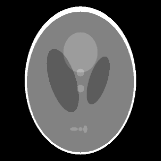
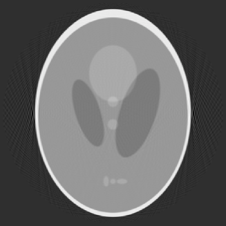
Figure 2. Reconstruction based on full data

The left figure is the original phantom. The right figure is the reconstruction by OPED based on the full data with $N=502$, which means 251 views with angles equally distributed over $[0,\pi]$ and 251 rays per view, and the size of the reconstruction is $256\times 256$ pixels. Reconstruction based on the full data has been discussed in [4, 20, 21], we will not give further details here as our purpose is to demonstrate the feasibility of our method on the limited angle problem.

For the reconstruction on the limited angle data, we choose the same set-up, with 201 angles over $[0,\pi]$ and 201 equally spaced parallel rays in each view.

In our first example, $r=21$, which amounts to data limited in an angle of about $165^{\circ}$; in other words, views from about $15^{\circ}$ angle are missing. The reconstruction by our algorithm is given in Figure 3 in which $\beta=0.9$ and $\tau=0$ for the left figure and $0.2$ for the right figure.

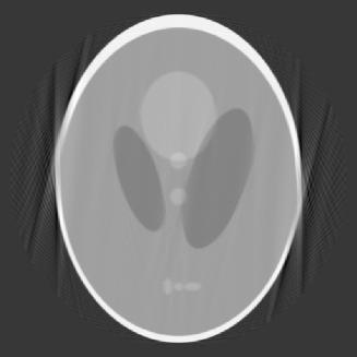
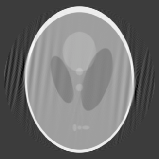
Figure 3. Reconstruction with $r=21$. Left: $\tau=0$  Right: $\tau=0.2$

The left image is reconstructed with $\tau=0$ and $\beta=0.9$; it is a fairly accurate reconstruction, although there are noticeable artifacts in the direction of missing views and a bit distortion around two spots on the edges. The right image is reconstructed with $\tau=0.2$ and $\beta=0.9$; it shows clearly artifacts of ripples, but the image appears to be sharper and has less distortion than the one in the left otherwise. In the case of $\tau=0$, the maximum of the condition numbers of the matrices $A_{k,r}^{(N)}$ is 160, so that the matrices are rather well conditioned. In the case of $\tau=0.2$, the maximum of the conditions numbers is $48928$, which may have contributed to the ripples in the image.

The condition that guarantees the non-singularity of the matrices in this case is $\tau<1-42/502\approx 0.916335$, whereas our computation of eigenvalues shows that $\tau$ has to be much smaller in order that the matrices are well conditioned. For our other examples, we will mostly take $\tau=0$. The choice of $\beta=0.9$ means that our sampling of coefficients follows a curve that decreases from 1 to 0.9, a decline that is rather mild, which leads to reasonable reconstruction image.

In our next example, we consider the case $r=42$, which means that the data is limited to views with angles distributed over an arc of $150^{\circ}$. The reconstruction with $\tau=0$ and $\beta=0.9$ is given in Figure 4.

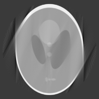
Figure 4. Reconstruction when $r=42$.

In this image, artifacts and distortion are clearly visible and most prominent at two points on the edges of the images. The maximum of the conditional numbers in this case is merely 503, so that the matrices are in fact fairly well conditioned. This suggests that the distortion is likely caused by the choice of $\tau=0$, which means that no polynomial preservation is kept.

4.2. Data with noise

The limited angle problem is well known to be ill-posed. Below we present our reconstruction with noise data. We use again the Shepp-Logan head phantom but add noise in the data, which is Gaussian normally distributed with zero mean and a standard deviation 0.03. The noise is about 2% in the data. For limited angle, we choose $r=21$ and $42$, respectively, which correspond to data limited over an arc of $165^{\circ}$ and $150^{\circ}$, respectively. The reconstructed images by our algorithm with $\tau=0$ and $\beta=0.9$ are given in Figure 5.

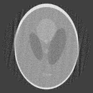
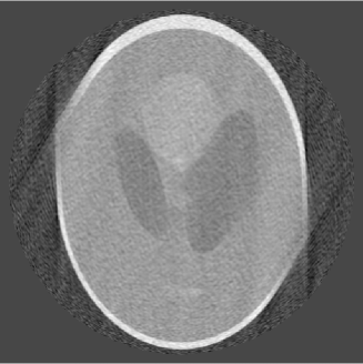
Figure 5. Noise data. Left: $r=21$. Right: $r=42$

These reconstruction should be compared with the left image in Figure 3 and the image in Figure 4, respectively, which are the reconstructed images based on the same limited angle data but without noise. These images indicate that our method is relatively stable, in the sense that the reconstructed images are not distorted much by the noise.

4.3. Discussion

The theoretic study and the numerical experiments point out that the proposed algorithm depends critically on the choice of $\tau$. The matrices remain relatively well conditioned for $\tau=0$ even when $r$ is large, but the case $\tau=0$ introduces distortion in the images, in addition to the artifacts. The reconstruction with $\tau>0$ appears to lead to less distortion in the images. However, the maximum of the condition numbers appears to grow exponentially with $r$ for $\tau>0$ and it increases drastically still for larger $\tau$. The ill-postedness of the matrices likely reflects the ill-posed nature of the limited angle problem. It is likely that solving the linear systems with pre-conditioning algorithms may improve the reconstructed images. This is, however, beyond the scope of the present paper.

5. Conclusion

A method for reconstruction images in the limited angle problem is presented and a theoretic study is carried out. The ill-posed nature of the problem shows up, when $\tau$ is not zero, in the ill-condition of the linear systems of equations that we need to solve. Numerical tests have demonstrated the feasibility of the method.

In order to fully understand the proposed method, further numerical study needs to be carried out. One interesting question is how much of the artifacts and the distortions are due to the ill-conditioning of the matrices when $\tau$ is not too small. The theoretic study indicates that the algorithm should be applied with $\tau$ relatively large if the severely ill-conditioned systems can be solved. On the other hand, as the limited angle problem is intrinsically ill-posed, there will have to be distortion of images when the angle is small.

References

- [1] B. Bojanov and I. K. Georgieva, Interpolation by bivariate polynomials based on Radon projections, Studia Math, 162 (2004), 141 - 160.
- [2] M. E. Davison, The ill-conditioned nature of the limited angle tomography problem, SIAM J. Applied Math. 43, (1983), 428 - 448.
- [3] C. F. Dunkl and Yuan Xu, Orthogonal polynomials of several variables, Cambridge Univ. Press, Cambridge, 2001.
- [4] H. de las Heras, O. Tischenko, Y. Xu and C. Heoschen, Comparison of the interpolation functions to improve a rebinning-free CT-reconstruction algorithm, Z. Med. Physik 18 (2008), 7-16.
- [5] J. Hsieh, Computed Tomography: principles, design, artifacts, and recent advances, SPIE Press Monograph Vol. PM114, Bellingham, Washington, 2003, p. 82-83.
- [6] A. Kak and MSlaney, Principles of Computerized Tomographic Imaging? IEEE Press 1988, reprinted by SIAM, Philadelphia, 2001.
- [7] B. F. Logan and L. A. Shepp, Optimal reconstruction of a function from its projections, Duke Math. J., 42:4, 1975, 645-659.
- [8] A. K. Louis, Approximation of the Radon transform from samples in limited range. Mathematical aspects of computerized tomography (Oberwolfach, 1980), 127–139, Lecture Notes in Med. Inform., 8, Springer, Berlin-New York, 1981.
- [9] A. K. Louis, Incomplete data problems in x-ray computerized tomography I. Singular value decomposition of the limited angle transform Numer. Math. 48 (1986), 251-262.
- [10] A. K. Louis, Development of algorithms in computerized tomography, in The Radon transform, inverse problems, and tomography, 25–42, Proc. Sympos. Appl. Math., 63, Amer. Math. Soc., Providence, RI, 2006.
- [11] A. Louis A and A. Rieder, Incomplete data problems in x-ray computerized tomography II. Truncated projections and region-of-interest tomography, Numer. Math. 56 (1989) 371 383.
- [12] R. Marr, On the reconstruction of a function on a circular domain from a sampling of its line integrals, J. Math. Anal. Appl., 45, 1974, 357-374.
- [13] F. Natterer, The mathematics of computerized tomography, Classics in Applied Mathematics, vol. 32, SIAM, Philadephia, 2001.
- [14] P. Petrushev, Approximation by ridge functions and neural networks, SIAM J. Math. Anal. 30 (1999), 155-189.
- [15] E. T. Quinto, Exterior and limited-angle tomography in non-destructive evaluation, Inverse Problems 14 (1998) 339-353.
- [16] D. Slepian, Prolate spheroidal wave functions, Fourier analysis, and uncertainty, V: the discrete case, Bell Sys. Tech. J. 57 (1978), 1371-1430.
- [17] L. Shepp and B. Logan, The Fourier reconstruction of a head section, IEEE Trans. Nucl. Sci., NS-21, 1974, 21-43.
- [18] Yuan Xu, Weighted approximation of functions on the unit sphere, Const. Approx., 21, 1-28.
- [19] Yuan Xu, A direct approach to the reconstruction of images from Radon projections, Adv. in Applied Math., 36, (2006), 388-420.
- [20] Yuan Xu and O. Tischenko, Fast OPED algorithm for reconstruction of images from Radon data, East. J. Approx. 12 (2007), 427-444.
- [21] Yuan Xu, O. Tischenko and C. Hoeschen, A new reconstruction algorithm for Radon Data, Proc. SPIE, Medical Imaging 2006: Physics of Medical Imaging, vol. 6142, p. 791-798.