Ultrashort pulse propagation and the Anderson localization

Abstract

We investigate the dynamics of a $10$ fs light pulse propagating in a random medium by the direct solution of the 3D Maxwell equations. Our approach employs molecular dynamics to generate a distribution of spherical scatterers and a parallel finite-difference time-domain code for the vectorial wave propagation. We calculate the disorder-averaged energy velocity and the decay time of the transmitted pulse Versus the localization length for an increasing refractive index.

As originally discussed by Anderson Anderson57 , and more recently in several articles john84 ; Kaveh ; Ishimaru84 ; Albada85 ; Maret ; Wiersma97 ; Johnson03 ; Pinheiro04 ; Lubatsch05 ; Wiersma07 ; Skipetrov07 ; toninelli:08 ; Conti08 , including Bose-Einstein condensation Billy08 ; Inguscio08 , elastic networks Hu08 , and optical beams Segev07 , three-dimensional (3D) wave localization may occur in the presence of structural randomness. An interesting issue is the role of localized states in the propagation of ultrashort laser pulses in random media Calba:08 , eventually including nonlinear effects Conti07 .

In this Letter we report on ab-initio computational results of ultra-short pulses in random media with increasing refractive index. Our approach combines Molecular Dynamics (MD) and parallel Finite-Difference Time-Domain (FDTD) codes: the former to provide realistic 3D distributions of scatterers with quenched disorder, the latter to exactly solve the vectorial Maxwell equations Conti07 . With such MD-FDTD technique, we study the propagation of classical waves in 3D disordered dielectrics for a varying scattering strength, as obtained by changing the scatterer refractive index $n$. As $n$ grows, the effective optical path increases and localization occurs. In what follows, we characterize the degree of localization of the electromagnetic (EM) field by the inverse participation ratio $\xi$ of the 3D energy profile and relate it to the transmission delay (expressed in terms of the energy velocity $v_{e}$) and to the decay constant of the trailing edge of the transmitted pulse (expressed in terms of an effective diffusion coefficient $D$). As the strong-localization regime is attained, $D$ and $v_{E}$ decrease; in addition the spectrum of the transmitted pulse displays several narrow peaks. By relating $v_{E}$ to $\xi$, we observe a signature of a transition, above which localized states are present.

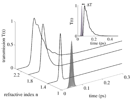
Figure 1: (Color online). Transmitted pulse $T(t)$ in linear scale for increasing refractive index $n$; the filled region is the adopted input pulse. $T(t)$ is scaled to unitary peak value for any $n$. The inset shows the time delay $\Delta T$ used to evaluate the energy propagation velocity $v_{E}$.

Our sample is a distribution of 1000 spherical scatterers obtained by MD simulations. Particle dimensions are chosen in order to match typical samples used in experiments, as e.g. in Vellekoop05 ; Storzer06 . We use a $50/50$ mixture of particle diameters $310$ nm and $248$ nm interacting with a generalized Lennard-Jones potential Conti07 ; at a filling fraction $\phi\cong 0.6$, this results in a largely disordered and tightly packed particle distribution in a cube with edge $L=2.9~{}\mu$m. The refractive index of the scatterers $n$ is chosen in the experimentally accessible range between $1.2$ and $2.8$. Several MD runs furnish different configurations of the disorder.

For each realization, we solve the Maxwell equations by a parallel FDTD algorithm TafloveBook and study the transmission of a Gaussian TEM₀₀ linearly $y-$polarized input pulse, with waist $w_{0}=1~{}\mu$m, impinging on the $xy$ face of the cube at normal incidence. The input pulse temporal profile is also Gaussian, with duration $t_{0}=10$ fs and carrier wavelength $\lambda_{0}=532$ nm. Numerical results have been averaged over five MD configurations of the $1000$ colloidal particles.

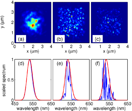
Figure 2: (Color online). (a-c) spatial distribution of the energy at the output face of the sample (at $t=0.5$ ps for a CW excitation at $\lambda=532$ nm). (d-f) spectrum of the electric field $E_{y}$ (thin line) calculated for $n=1.4$, $2.2$ and $n=2.8$; the thick line is the spectrum of the incident pulsed beam.

For each set of MD-FDTD simulations we collect: i) the total transmission $T(t)$ by integrating the $z-$component of the Poynting vector with respect to the transverse ($x,y$) output plane, ii) the $y-$component of the output electric field $E_{y}$, iii) the corresponding spectrum and iv) the EM energy density $\mathcal{E}$. In addition, we calculate the distribution of decay times $g(\tau)$:

$$T(t)=\int_{0}^{\infty}e^{-t/\tau}g(\tau)d\tau,$$ (1)

by a best-fit with a superposition of exponentially decaying functions. The mean value $\bar{\tau}$ for the decay-time is then used to calculate the “effective” light diffusion constant as $D=L^{2}/\pi^{2}\bar{\tau}$ (in the broadband short-sample regime here considered the diffusion approximation is not expected to be strictly valid).The energy propagation velocity $v_{E}$ is calculated by determining the time $\Delta T$ spent by the pulse peak (from the Poynting vector) to travel from the input to the output face of the sample (see inset in Fig. 1), letting $v_{E}=L/\Delta T$, and averaging over disorder realization.
To characterize the localization length, we calculate the inverse participation ratio $\xi$:

$$\xi=\sqrt[3]{\frac{(\int_{V}\mathcal{\mathcal{E}}^{2}(x,y,z)dV)^{2}}{\int_{V}\mathcal{\mathcal{E}}^{4}(x,y,z)dV}},$$ (2)

being $V=L^{3}$ the sample volume. $\xi$ is such that if the energy profile decays as an exponential with decay constant $l_{\xi}$, it is $\xi=2l_{\xi}$; hence it directly measures the spatial extension of $\mathcal{E}(x,y,z)$. $\xi$ is calculated by using a continuous wave (CW) beam at $\lambda=532$ nm, to avoid the simultaneous excitation of several modes.

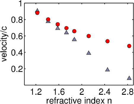
Figure 3: (Color online). Phase $v_{p}$ (circles) and energy $v_{E}$ (triangles) velocity versus $n$.

Figure 1 shows the input (filled region) and the transmitted pulses $T(t)$ (solid lines), for increasing values of $n$; the $T(t)$ tail gets longer due to the reduced light diffusivity $D$, while the transmitted pulse slows down (see figure 3 below). As shown in Fig. 2a-c, spatial distribution of the energy $\mathcal{E}$ radically changes from extended $(n=1.4)$ to localized states $(n=2.2$ and $n=2.8)$. Correspondingly, the spectrum of $E_{y}$ splits into multiple modes (Fig. 2d-f), which implies longer lifetimes for the involved EM resonances and a dynamic slowing down (Fig. 1).

In Fig. 3 we compare the trend of $v_{E}$ (triangles) versus $n$ with that of the corresponding phase velocity $v_{p}$ (circles), which is calculated as $v_{p}\simeq c/\bar{n}$ [being $\bar{n}=\phi~{}n+(1-\phi)$, the mean refractive index of the colloidal spheres dispersed in air]. The increase of the degree of localization is accompanied by the concurrent swelling of the discrepancy between $v_{E}$ and $v_{p}$, which becomes appreciable for $n$ greater than a critical value $n_{c}\cong 1.8$. Previous experimental investigations have reported significant deviations from an exponential transmission for an average index $\bar{n}=1.55$ Storzer06 ; in our case we have as the critical value for the localization $\bar{n}=1.48$. However further work is required for a strict quantitative comparison with experiments.

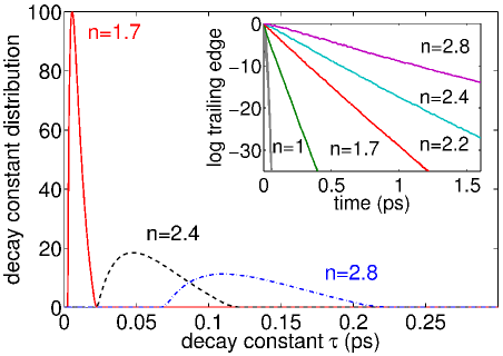
Figure 4: (Color online). Distribution of decay-times of the trailing edge of the transmission $T$ for various $n$. The inset shows the log-scale plot of normalized transmitted signals $T(t)$ (trailing edge).

Figure 4 shows the decay constant distribution $g(\tau)$ of trailing edge of the transmission $T(t)$, as calculated from Eq. (1). The inset of Fig. 4 shows the trailing edge of the scaled and temporally shifted transmitted pulse in logarithmic scale; the reported linear trends apparently indicate the absence of any sensible deviation from a single exponential, which however becomes evident from the spreading of $g(\tau)$. Note that at the localization, the width of $g(\tau)$ is comparable to its mean value $\bar{\tau}$.

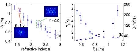
Figure 5: (Color online).(a) Localization length $\xi$ versus refractive index $n$; the error bars and average values as calculated over $5$ realizations of the disorder. The two insets show the snapshot of the energy profile at the output face of the sample for two values of $n$. (b)Parametric plot (versus $n$) of the ratio $v_{p}/v_{e}$ (left scale) and of $D$ (right scale) versus $\xi$.

Figure 5a shows the participation ratio $\xi$ for different values of the refractive index $n$. As expected the EM resonances become more localized as the optical path in each scatterer increases; however since $\xi$ is a volume averaged quantity, it does not display a discontinuous trend versus $n$. In Fig. 5b we draw the ratio between phase and energy velocity $v_{p}/v_{E}$ and the dynamic diffusion $D$ versus $\xi$. This analysis yields a crossover at $\xi(n_{c})$, where the discrepancy between $v_{E}$ and $v_{p}$ is evident. Beyond the threshold the reduction of the localization length is accompanied by the slowing down of the pulse and a simple one-to-one relation between $\xi$ and $v_{E}$ is evident. It is important to stress that $D$ is expected to vanish at the Anderson transition for an infinitely extended structure; here we find that, for finite size systems, $D$ (and the energy velocity $v_{E}$) directly measures the degree of spatial localization.

In conclusion we reported on what we believe to be the first time-resolved analysis of ultra-short light pulses in 3D disordered samples. Our approach combines molecular dynamics and finite-difference time-domain codes, thus providing a realistic distribution of the scatterers and an exact theory of wave propagation. The distribution of the decay-time is shown to largely spread at the Anderson transition. The plot of the ratio between the energy and the phase velocity versus the localization length displays a critical character; the more localized are the excited EM resonances, the slower is the input pulse propagation. The diffusion constant is not vanishing at the localization transition and it is a direct measure of the spatial extension of the EM field. These findings are expected to stimulate novel theoretical works and experiments in the large community dealing with energy propagation in the presence of disorder, ranging from optics to quantum systems.
Acknowledgments. — The research leading to these results has received funding from the European Research Council under the European Community’s Seventh Framework Program (FP/2007-2013)/ERC grant agreement n. 201766. We acknowledge support to INFM-CINECA and CASPUR for the initiative for parallel computing.

References

- (1) P. Anderson, Phys. Rev. 109, 1492 (1958).
- (2) S. John, Phys. Rev. Lett. 53, 2169 (1984).
- (3) M. Kaveh, Phil. Mag. B 56, 693 (1987).
- (4) L. Tsang and A. Ishimaru, J. Opt. Soc. Am. A1, 836 (1984).
- (5) M. Albada and A. Lagendijk, Phys. Rev. Lett. 55, 2692 (1984).
- (6) P. Wolf and G. Maret, Phys. Rev. Lett. 55, 2692 (1985).
- (7) D. S. Wiersma, P. Bartolini, A. Lagendijk, and R. Righini, Nature 390, 671 (1997).
- (8) P. M. Johnson, A. Imhof, B. P. J. Bret, J. G. Rivas, and A. Lagendijk, Phys. Rev. E68, 016604 (2003).
- (9) F. A. Pinheiro, M. Rusek, A. Orlowski, and B. A. Tiggelen, Phys. Rev. E 69, 026605 (2004).
- (10) A. Lubatsch, J. Kroha, and K. Busch, Phys. Rev. B71, 184201 (2005).
- (11) R. Sapienza, P. García, J. Bertolotti, M. D. Martín, A. Blanco, L. Vina, C. López, and D. Wiersma, Phys. Rev. Lett. 99, 233902 (2007).
- (12) S. E. Skipetrov and B. A. Tiggelen, Phys. Rev. Lett. 96, 043902 (2006).
- (13) C. Toninelli, E. Vekris, G. A. Ozin, S. John, and D. S. Wiersma, Physical Review Letters 101, 123901 (2008).
- (14) C. Conti and A. Fratalocchi, Nat.Phys. 4, 794 (2008).
- (15) J. Billy, V. Josse, Z. Zuo, A. Bernard, B. Hambrecht, P. Lugan, D. Clement, L. Sanchez-Palencia, P. Bouyer, and A. Aspect, Nature 453, 891 (2008).
- (16) G. Roati, C. D’Errico, L. Fallani, M. Fattori, C. Fort, M. Zaccanti, G. Modugno, M. Modugno, and M. Inguscio, Nature 453, 895 (2008).
- (17) H. Hu, A. Strybulevych, J. H. Page, S. E. Skipetrov, and B. A. Van Tiggelen, arXiv:0805.1502 (2008).
- (18) T. Schwartz, G. Bartal, S. Fishman, and M. Segev, Nature 446, 52 (2007).
- (19) C. Calba, L. Méès, C. Rozé, and T. Girasole, J. Opt. Soc. Am. A 25, 1541 (2008).
- (20) C. Conti, L. Angelani, and G. Ruocco, Phys. Rev. A75, 033812 (2007).
- (21) I. M. Vellekoop, P. Lodahl, and A. Lagendijk, Phys. Rev. E71, 056604 (2005).
- (22) M. Storzer, P. Gross, C. M. Aegerter, and G. Maret, Phys. Rev. Lett. 96, 063904 (2006).
- (23) A. Taflove and S. C. Hagness, Computational Electrodynamics: the finite-difference time-domain method (Artech House, 2000), 3rd ed.