Gravitational collapse of radiation fluid in higher dimensions

Abstract

Abstract: We examine the problem of the gravitational collapse using higher dimensional Husain spacetime for the null fluid. The equations of state chosen to solve the field equations contain linear, quadratic and arbitrary powers of the radial parameter. The resulting mass evolution is discussed for each case.

Keywords: Accretion; Black Hole; General Relativity; Gravitational Collapse

I Introduction

The problem of gravitational collapse of massive bodies is fascinating and a long standing one in general relativity. This problem arises since general relativity predicts vanishing pressure gradients against daunting gravitational forces in massive objects (of the order of solar masses). Generally, spherically symmetrical object of mass $M$ and radius $r$ related by $r\sim 2M$ (in units $c=G=1$), undergoes unrestricted collapse penrose . This process may not be spherically symmetrical if the collapsing object possesses angular momentum. The theory of gravitational collapse has been widely studied. Examples are: Collapse of a massive dust cloud snyder , charged perfect fluid sphere mashoon , rotating massive body wagoner ; cohen , role of bulk viscosity during collapse nakia ; herrera , collapse in the background of cosmological constant shapiro , thin spherical shell of dust israel , collapse of homogeneous scalar fields roberto and collapse in higher dimensional spacetimes bizon ; goswami .

Almost all the gravitational collapse models lead to the formation of spacetime singularities generally hidden by one or more horizons. A singularity is a region where invariants like Kretschman scalar and curvature scalar diverge. Numerical simulations of gravitational collapse of spheroids show that if the collapsing spheroid is sufficiently compact, the singularities are hidden inside the event horizon while they become naked (devoid of event horizon) if the spheroid is sufficiently large shapiro1 . However, there are some models in which the formation of singularity is avoided e.g. if the collapsing star radiates all the matter torres . Another such model is that of a ‘regular phantom black hole’ which contains Schwarzschild like causal structure and the singularity is replaced by the de Sitter infinity bronn1 .

There has been huge interest in naked singularities, although their existence is not very clear and these are prohibited by the cosmic censorship hypothesis patel . The existence and formation of naked singularities has been suggested for the gravitational collapse in self-similar spacetimes lake . The visibility of a singularity is possible if there exists a null geodesic emanating from the singularity. Then it requires the existence of families of future directed non-spacelike curves which emanate from the vicinity of the singularity joshi . The observation of these non-spacelike curves will give sufficient information about the singularity itself. Such a mysterious singularity can also be observable if sufficiently strong shearing effects near the singularity delay the formation of the event horizon joshi1 . Another such possibility is that of a black hole accreting phantom energy which results in its ‘evaporation’ and leading to a naked singularity babichev ; jamil ; jamil1 ; jamil2 ; jamil3 . Astrophysically, the phenomenon of gravitational collapse is manifested in the form of a gamma ray burst in which a super-giant star explodes and releases immense heat flux while the stellar core collapses to form a black hole remanent zhe .

The problem of spherical collapse of a null fluid has been studied earlier by Husain viqar and recently extended to higher dimensions by Debnath et al debnath . We here investigate the same problem using equations of state which are more general than the barotropic EoS $p=\omega\rho$. These EoS yield interesting behaviors for the evolution of mass of the black hole.

II Modeling of system

We assume an ($n+2$)-dimensional spherically symmetric Husain spacetime given by debnath

$$ds^{2}=-\left(1-\frac{m(v,r)}{r^{n-1}}\right)dv^{2}+2dvdr+r^{2}d\Omega_{n}^{2},$$ (1)

where the radial coordinate is restricted in the range $0<r<\infty$ and the advanced null coordinate $v=t-r$ with $-\infty\leq v\leq\infty$ is called the Eddington coordinate. Here we have the energy momentum tensor with two components: null radiation fluid and the matter fluid i.e.

$$T_{\mu\nu}=T_{\mu\nu}^{(n)}+T_{\mu\nu}^{(m)},$$ (2)

where

$$T_{\mu\nu}^{(n)}=\sigma l_{\mu}l_{\nu},$$ (3)

and

$$T_{\mu\nu}^{(m)}=(\rho+p)(l_{\mu}\eta_{\nu}+l_{\nu}\eta_{\mu})+pg_{\mu\nu}.$$ (4)

Everywhere in this paper, all Greek indices range from 1 to $n+2$. Here $l^{\mu}=(1,0,0,...,0)$, and $\eta_{\mu}=\left(\frac{1}{2}\left(1-\frac{m}{r^{n-1}}\right),-1,0,...,0\right)$, are future-like Null vectors, satisfying $l_{\lambda}l^{\lambda}=\eta_{\lambda}\eta^{\lambda}=0$, and $l_{\lambda}\eta^{\lambda}=-1$. Also $\sigma$ is the is the energy density corresponding to the Vaidya null direction. We require the energy momentum tensor to satisfy the energy conditions given by (a) Weak and strong energy conditions are: $\sigma>0,\ \rho\geq 0,\ p\geq 0$. (b) Dominant energy condition (DEC) is: $\sigma>0,\ \rho\geq p,\ p\geq 0$.

The Einstein field equations are

$$G_{\mu\nu}=T_{\mu\nu},$$ (5)

for the metric (1) with matter field having stress-energy tensor given by

$$\rho = \frac{nm^{\prime}}{2r^{n}},$$ (6)

$$p = -\frac{m^{\prime\prime}}{2r^{n-1}},$$ (7)

$$\sigma = \frac{n\dot{m}}{2r^{n}}.$$ (8)

Here prime ^′ and overdot . denote differentiation with respect to the parameters $r$ and $v$ respectively. For the positive definiteness of $\rho$, $p$ and $\sigma$, we require

$$(a)\ m^{\prime}\geq 0,\ m^{\prime\prime}\leq 0\ and\ \ (b)\ \dot{m}>0.$$ (9)

We take the following cases of equations of state to solve the field equations (6) - (8):

1. $p(v)=-Ar+B\rho(v)$,

2. $p(v)=(Dr+Er^{2})\rho(v)$,

3. $p(v)=Cr^{k}\rho(v)$.

Here $A$, $B$, $C$, $D$ and $E$ are arbitrary constants independent of both $r$ and $v$. Note that the barotropic EoS $p=\omega\rho$, represents an asymptotically flat spacetime if the parameter $\omega$ is constrained by $\frac{1}{2}<\omega\leq 1$, while $\omega=1$ represents a charged Vaidya solution viqar .

II.1 Case-1: EoS Linear in $r$

We consider an EoS which is linear in variable $r$ and is given by

$$p(v)=-Ar+B\rho(v),$$ (10)

Using Eqs. (6), (7) and (10), we get

$$m^{\prime\prime}(r,v)=2Ar^{n}-\frac{nBm^{\prime}(r,v)}{r}.$$ (11)

Solving Eq. (11), we obtain

$$m(r,v)=C_{1}(v)+C_{2}(v)\frac{r^{1-Bn}}{1-Bn}+\frac{2Ar^{2+n}}{(2+n)(1+n+Bn)},$$ (12)

where $C_{1}(v)$ and $C_{2}(v)$ are arbitrary functions of time $v$. Differentiating Eq. (12), w.r.t $r$ yields

$$m^{\prime}(r,v)=C_{2}(v)r^{-Bn}+\frac{2Ar^{n+1}}{1+n+Bn},$$ (13)

while second differentiation gives

$$m^{\prime\prime}(r,v)=-C_{2}(v)Bnr^{-1-Bn}+\frac{2A(n+1)r^{n}}{1+n+Bn}.$$ (14)

Also differentiation of Eq. (12) w.r.t $v$ gives

$$\dot{m}(r,v)=\dot{C}_{1}(v)+\dot{C}_{2}(v)\frac{r^{1-Bn}}{1-Bn}.$$ (15)

Now using Eq. (13) $m^{\prime}\geq 0$ $\Rightarrow$ $\frac{2Ar^{n+1}}{1+n+Bn}+r^{-Bn}C_{2}(v)\geq 0$. It yields

$$r\geq\left[-\frac{C_{2}(1+n+Bn)}{2A}\right]^{\frac{1}{1+n+Bn}}.$$ (16)

Now $-\frac{2A}{C_{2}(1+n+Bn)}\geq 0$ if either $A>0$ and $C_{2}(1+n+Bn)<0$ or vice-versa. The later quantity yields $C_{2}>0$ and $1+n+Bn<0$ and vice versa. Also $m^{\prime\prime}\leq 0$ implies

$$\frac{2A(n+1)r^{n}}{1+n+Bn}-Bnr^{-1-Bn}C_{2}(v)\leq 0,$$ (17)

which gives

$$r^{1+n+Bn}\leq Bn\frac{(1+n+Bn)}{2A(1+n)}.$$ (18)

Further, $\dot{m}>0$ implies

$$\dot{C}_{1}(v)+\dot{C}_{2}(v)\frac{r^{1-Bn}}{1-Bn}>0,$$ (19)

or

$$\frac{\dot{C}_{1}}{\dot{C}_{2}}>\frac{r^{1-Bn}}{Bn-1}.$$ (20)

Now horizon of the metric is obtained by $1-\frac{m(r,v)}{r^{n-1}}=0$. It implies $m(r,v)=r^{n-1}$ which further yields

$$C_{1}(v)+C_{2}(v)\frac{r^{1-Bn}}{1-Bn}+\frac{2Ar^{2+n}}{(2+n)(1+n+Bn)}=r^{n-1},$$ (21)

which is an algebraic equation in $r$.

In the graphs to follow, we plot the evolution of a black hole mass by considering different models (i.e. cases 1 to 3) resulting from the equations of state of a null fluid. Our graphs result from different choices of functions $C_{i}$, $i=1...6$ which are chosen quite arbitrarily including polynomial, trigonometric and the exponential functions, and exhibit various behaviors for the mass parameter $m$. These functions $C_{i}$, then lead to increasing, decreasing or fluctuating manner of mass.

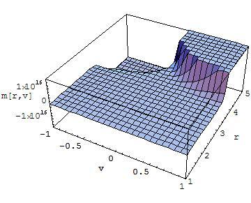
Figure 1: The mass $m(r,v)$ is plotted against $r$ and $v$ for the choice of functions $C_{1}$ and $C_{2}$.

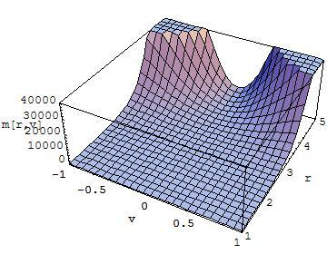
Figure 2: The mass $m(r,v)$ is plotted against $r$ and $v$ for the choice of functions $C_{1}$ and $C_{2}$.

In figure 1, we have chosen $C_{1}(v)=e^{v^{2}}$ and $C_{2}(v)=\sin v^{3}$. The constant parameters are fixed at $A=3$, $B=-8$ and $n=4$. It is shown that mass increases in steps as $r$ increases for $v>0$ whereas for $v<0$, the mass increases as $r$ decreases. In figure 2, the functions are chosen as $C_{1}(v)=e^{v^{2}}$ and $C_{2}(v)=\sin v^{2}$; while the constants are taken to be $A=-3$, $B=-2$ and $n=4$. The graph shows that this model is similar to the previous one except for the symmetry in $v$ i.e. the mass increases with the increases in radial coordinate $r$.

II.2 Case-2: EoS quadratic in $r$

We now take another EoS which is quadratic in $r$ given by

$$p(v)=(Dr+Er^{2})\rho(v).$$ (22)

The governing equation is

$$m^{\prime\prime}(r,v)=-n\left(D+Er\right)m^{\prime}(r,v).$$ (23)

Solving Eq. (23), we obtain

$$m(r,v)=C_{3}(v)+C_{4}(v)\exp\left(\frac{D^{2}n}{2E}\right)\sqrt{\frac{2}{\pi E}}\int\limits_{0}^{\sqrt{\frac{n}{2E}}(D+Er)}e^{-z^{2}}dz.$$ (24)

Also differentiation of Eq. (24) w.r.t $r$ gives

$$m^{\prime}(r,v)=C_{4}(v)\exp\left(-\frac{1}{2}nr(2D+Er)\right).$$ (25)

Substitution of (25) in (23) gives

$$m^{\prime\prime}(r,v)=-nC_{4}(v)(D+Er)\exp\left(-\frac{1}{2}nr(2D+Er)\right).$$ (26)

Differentiation of Eq. (24) w.r.t $v$ results

$$\dot{m}(r,v)=\dot{C}_{3}(v)+\dot{C}_{4}(v)\exp\left(\frac{D^{2}n}{2E}\right)\sqrt{\frac{2}{\pi E}}\int\limits_{0}^{\sqrt{\frac{n}{2E}}(D+Er)}e^{-z^{2}}dz.$$ (27)

Now $m^{\prime}(r,v)\geq 0$ $\Rightarrow C_{4}(v)\exp(-\frac{1}{2}nr(2D+Er))\geq 0$ $\Rightarrow C_{4}(v)\geq 0$. Further, $m^{\prime\prime}(r,v)\leq 0\Rightarrow-n(D+Er)C_{4}(v)\leq 0$, when $n(D+Er)\geq 0$. Also $\dot{m}(r,v)>0$ implies

$$\frac{\dot{C}_{3}(v)}{\dot{C}_{4}(v)}>-\exp\left(\frac{D^{2}n}{2E}\right)\sqrt{\frac{2}{\pi E}}\int\limits_{0}^{\sqrt{\frac{n}{2E}}(D+Er)}e^{-z^{2}}dz.$$ (28)

Now to calculate the horizon we take $m(r,v)=r^{n-1}$ which gives

$$C_{3}(v)+C_{4}(v)\exp\left(\frac{D^{2}n}{2E}\right)\sqrt{\frac{2}{\pi E}}\int\limits_{0}^{\sqrt{\frac{n}{2E}}(D+Er)}e^{-z^{2}}dz=r^{n-1}.$$ (29)

In figure 3, we have chosen $C_{3}(v)=e^{v^{3}}$ and $C_{4}(v)=\cot v^{2}$. The constant parameters are fixed at $D=2$, $E=3$ and $n=6$. Here the mass $m$ possesses symmetry about $v=0$. The mass eventually decreases for large $v$. In figure 4, the functions are chosen as $C_{3}(v)=e^{v}$ and $C_{4}(v)=\csc v^{2}$ with the same choice of constants as in Fig. 3. The mass decreases when $v$ increases except for the singularity at $v=0$.

II.3 Case-3: EoS with arbitrary power in $r$

Let us now take the EoS

$$p(v)=Cr^{k}\rho(v).$$ (30)

Here $C$ and $k$ are arbitrary constants. The governing differential equation is given by

$$m^{\prime\prime}(r,v)=-nCr^{k-1}m^{\prime}(r,v).$$ (31)

The solution of the above equation is

$$m(r,v)=C_{5}(v)-\frac{r}{k}C_{6}(v)\left(\frac{Cnr^{k}}{k}\right)^{-\frac{1}{k}}\Gamma\left(\frac{1}{k},\frac{Cnr^{k}}{k}\right),$$ (32)

where we have an incomplete Gamma function given by

$$\Gamma\left(\frac{1}{k},\frac{Cnr^{k}}{k}\right)=\int\limits_{\frac{Cnr^{k}}{k}}^{\infty}x^{\frac{1}{k}-1}e^{-x}dx.$$ (33)

Differentiation of Eq. (32) w.r.t $r$, we have

$$m^{\prime}(r,v)=C_{6}(v)\exp\left(-\frac{Cnr^{k}}{k}\right).$$ (34)

Again differentiating yields

$$m^{\prime\prime}(r,v)=-Cnr^{k-1}C_{6}(v)\exp\left(-\frac{Cnr^{k}}{k}\right).$$ (35)

Further differentiation w.r.t $v$ gives

$$\dot{m}(r,v)=\dot{C}_{5}(v)-\frac{r}{k}\dot{C}_{6}(t)\left(\frac{Cnr^{k}}{k}\right)^{-\frac{1}{k}}\Gamma\left(\frac{1}{k},\frac{Cnr^{k}}{k}\right),$$ (36)

Now $m^{\prime}(r,v)\geq 0$ implies $C_{6}(v)\geq 0$. Also $m^{\prime\prime}(r,v)\leq 0$ implies $-Cnr^{k-1}C_{6}(v)\exp(-\frac{Cnr^{k}}{k})\leq 0$, hence $Cnr^{k-1}C_{6}(v)\geq 0$. Further $\dot{m}(r,v)>0$ implies

$$\frac{\dot{C}_{5}(v)}{\dot{C}_{6}(v)}>\frac{r}{k}\left(\frac{Cnr^{k}}{k}\right)^{-\frac{1}{k}}\Gamma\left(\frac{1}{k},\frac{Cnr^{k}}{k}\right).$$ (37)

Now horizon of the spacetime is obtained by solving

$$C_{5}(v)-\frac{C_{6}(v)r}{k}\left[\left(\frac{Cnr^{k}}{k}\right)^{-\frac{1}{k}}\Gamma\left(\frac{1}{k},\frac{Cnr^{k}}{k}\right)\right]=r^{n-1}.$$ (38)

In figure 5, we have chosen $C_{5}(v)=e^{v^{2}}$ and $C_{6}(v)=v^{4}$. The constant parameters are fixed at $c=2$, $k=6$ and $n=3$. In figure 6, the functions are chosen as $C_{5}(v)=e^{v^{3}}$ and $C_{6}(v)=v^{3}$ with the same choice of constants as in Fig. 5. The mass increases as $v$ increases in both cases. Thus the accretion of the null fluid results in the increase in mass of the black hole.

Also note that the dominant energy condition $\rho\geq p$ implies

$$r\geq-\frac{nm^{\prime}}{m^{\prime\prime}}.$$ (39)

which is a general expression. For $p=-Ar+B\rho$, it gives

$$r\geq-n\left[\frac{2Ar^{n+1}+c_{1}r^{-Bn}(1+n+Bn)}{2A(n+1)r^{n}-c_{1}Bnr^{-1-Bn}(1+n+Bn)}\right].$$ (40)

For $p=(Dr+Er^{2})\rho(t)$, the condition Eq. (39) leads to

$$r\geq\frac{1}{D+Er}.$$ (41)

It further gives $(D+Er)r\geq 1\Rightarrow r\geq 1$ and $(D+Er)r\geq 1$. The later yields $r\geq\frac{1-D}{E}$.

In the third case, $p=Cr^{k}\rho(t)$ the DEC implies

$$r\geq\frac{1}{Cr^{k-1}}\Rightarrow r\geq\left(\frac{1}{C}\right)^{\frac{1}{k}}.$$ (42)

III Conclusion

In this paper, we have investigated the gravitational collapse model of higher dimensional Husain spacetime. We have obtained three different expressions of mass in the corresponding three cases. These expressions contain certain functions $C_{i}$ which needs to be chosen arbitrarily since no boundary conditions are imposed on the governing dynamical equations. However our choices of these functions lead to some interesting results: In cases 1 and 3, the mass of black hole is increasing due to accretion of null fluid. These solutions physically describe the inward (ingoing) Husain spacetime poisson . However the solutions obtained in case-2 describe the outward (outgoing) Husain spacetime since the mass is decreasing. Our solutions also satisfy the weak and dominant energy conditions which are necessarily satisfied in the classical gravity. Moreover, the equations of state chosen here, are generalizations of the previously used ones in viqar and hence give a much deeper understanding of the process.

Acknowledgment

We would like to thank Viqar Husain, Ujjal Debnath and Alberto Saa for useful correspondence related to this work.

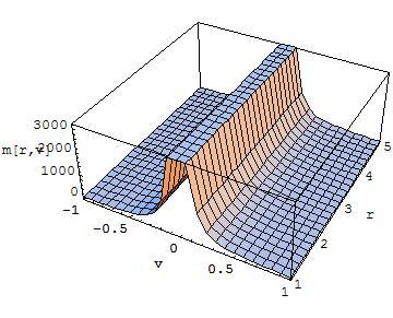
Figure 3: The mass $m(r,v)$ is plotted against $r$ and $v$ for the choice of functions $C_{3}$ and $C_{4}$.

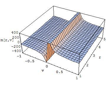
Figure 4: The mass $m(r,v)$ is plotted against $r$ and $v$ for the choice of functions $C_{3}$ and $C_{4}$.

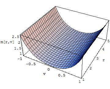
Figure 5: The mass $m(r,v)$ is plotted against $r$ and $v$ for the choice of functions $C_{5}$ and $C_{6}$.

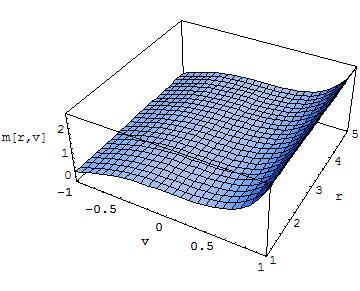
Figure 6: The mass $m(r,v)$ is plotted against $r$ and $v$ for the choice of functions $C_{5}$ and $C_{6}$.

References

- (1) R. Penrose, Gen. Relativ. Gravit. 34 (2002) 1141.
- (2) W.B. Oppenheimer and H. Snyder, Phys. Rev. 56 (1939) 455.
- (3) B. Mashoon and M.H. Partovi, Phys. Rev. D 20 (1979) 2455.
- (4) R.V. Wagoner, Phys. Rev. 138 (1965) 1583.
- (5) J.M. Cohen, Phys. Rev. 173 (1968) 1258.
- (6) N. Carlevaro and G. Montani, Class. Quant. Grav. 22 (2005) 4715.
- (7) L. Herrera et al, gr-qc/0804.3584v1.
- (8) D. Markovic and S.L. Shapiro, Phys. Rev. D 61 (2000) 084029.
- (9) W. Israel, Phys. Rev. 153 (1967) 1388.
- (10) R. Giambo, Class. Quant. Grav. 22 (2005) 2295.
- (11) P. Bizon et al, Phys. Rev. D 72 (2005) 121502R.
- (12) R. Goswami and P.S. Joshi, Phys. Rev. D 76 (2007) 084026.
- (13) S.L. Shapiro and S.A. Teukolsky, Phys. Rev. Lett. 66 (1991) 994.
- (14) F. Fayos and R. Torres, Class. Quant. Grav. 25 (2008) 175009.
- (15) K.A. Bronnikov and J.C. Fabris, Phys. Rev. Lett. 96 (2006) 251101.
- (16) K.D. Patel et al, Chin. Phys. Lett. 25 (2008) 854.
- (17) K. Lake and T. Zannias, Phys. Rev. D 41 (1990) 3866R.
- (18) P.S. Joshi, Phys. Rev. D 75 (2007) 044005.
- (19) P.S. Joshi et al, Phys. Rev. D 65 (2002) 101501.
- (20) E. Babichev et al, Phys. Rev. Lett. 93 (2004) 021102.
- (21) M. Jamil et al, Eur. Phys. J. C 58 (2008) 325
- (22) M. Jamil, Eur. Phys. J. C 62 (2009) 609
- (23) F. De Paolis et al, Int. J. Theor. Phys. DOI 10.1007/s10773-009-0242-4
- (24) M. Jamil, Il Nuovo Cimento B 123 (2008) 599
- (25) C. Zhe et al, Commun. Theor. Phys. 50 (2008) 271.
- (26) V. Husain, Phys. Rev. D 53 (1995) R1759
- (27) U. Debnath et al, Gen. Relativ. Gravit. 40 (2008) 749
- (28) E. Poisson, A Relativist’s Toolkit: The Mathematics of Black Hole Mechanics, Cambridge University Press, 2004.