VELOCITY DOMINATED SINGULARITIES IN THE CHEESE SLICE UNIVERSE

Abstract

We investigate the properties of spacetimes resulting from matching together exact solutions using the Darmois matching conditions. In particular we focus on the asymptotically velocity term dominated property (AVTD). We propose a criterion that can be used to test if a spacetime constructed from a matching can be considered AVTD. Using the Cheese Slice universe as an example, we show that a spacetime constructed from a such a matching can inherit the AVTD property from the original spacetimes. Furthermore the singularity resulting from this particular matching is an AVTD singularity.

1 Introduction

The Friedmann-Lemaître-Robertson-Walker (FLRW) [2, 3, 4, 5] spacetime is a good cosmological model with which to approximate our universe, but it does not account for inhomogeneities that are observed in small and large scale structure. In an attempt to model more realistic cosmologies that can account for large scale inhomogeneities there have been some models proposed that are constructed my matching together various solutions. The most famous of which is the Einstein-Straus “Swiss Cheese” models [6]. More recently there has been a planar model proposed by matching together FLRW and Kasner [7] spacetimes. In relation to the Einstein-Straus models, these models have been termed the “Cheese Slices” universe. Such constructions could be of interest in relation to the observed layering in the distribution of galaxies reported by Broadhurst et al. [8].

However, if such cosmologies are to be used as models of our universe, we must understand their implications at all stages of evolution including at the initial singularity. In particular, when a cosmology is constructed by matching together different spacetimes, what structure does the singularity inherit from the matching? Does a matching at late times naturally imply, in any sense, a “well behaved” matching at the singularity? Such questions are difficult to formulate in the most general terms, thus we choose to focus on the aspect of velocity dominated singularities.

Belinskii, Khalatnikov and Lifshitz (BKL) [9] have conjectured that in a generic singularity the evolution towards the singularity is independent of spatial curvature. Since then other authors have attempted to formulate more precise definitions of this property such as Eardley, Liang and Sachs [10] in their definition of velocity dominated singularities. Their definition has been generalized by Isenberg and Moncrief [11] and is known as the asymptotically velocity term dominated (AVTD) property.

In particular with the Cheese Slice universe, we have a matching of two AVTD spacetimes with asymptotically velocity term dominated singularities (AVTDS). The question arises of whether or not the singularity in the Cheese slice universe inherits the AVTD property from the spacetimes used in its construction. In section 2 we show how a spacetime constructed from a matching can be considered to be AVTD. We will also detail the Darmois matching conditions [12] that we adopt as our matching criteria throughout. Then in section 3 we show that the Cheese Slice singularity is indeed an AVTDS.

In the following Greek indexes indicate four dimensions, $\alpha,\beta,\gamma\ldots=\{0,1,2,3\}$. Latin indexes indicate three dimensions, $a,b,c\ldots=\{1,2,3\}$ and upper case indexes indicate two dimensions, $A,B,C\ldots=\{1,2\}$. We will also refer to spacetimes constructed by matching together different solutions as a “matched spacetime”.

2 The AVTD Property of a Matched Spacetime

2.1 Definitions

Let $U$ be a spacetime with metric $g_{\alpha\beta}$ and coordinates $x^{\alpha}$. We begin by choosing a spatial foliation with intrinsic coordinates $\xi^{a}$ on each leaf of the foliation. Next we identify the intrinsic metric,

$$\gamma_{ab}=\frac{\partial x^{\alpha}}{\partial\xi^{a}}\frac{\partial x^{\beta}}{\partial\xi^{b}}g_{\alpha\beta},$$ (1)

and extrinsic curvature,

$$K_{ab}=\frac{\partial x^{\alpha}}{\partial\xi^{a}}\frac{\partial x^{\beta}}{\partial\xi^{b}}\nabla_{\alpha}n_{\beta},$$ (2)

of the spacelike three surfaces, where $n_{\alpha}$ is the normal to the surface. The mean curvature is then $K=K^{a}_{a}$. The timelike foliation vector, $\partial/\partial t$, where $t$ is a timelike coordinate that labels successive leaves of the foliation, describes the evolution of the three surface and is related to the surface normal via the lapse $N$ and shift $M_{\alpha}$,

$$\frac{\partial}{\partial t}=Nn_{\alpha}+M_{\alpha}.$$ (3)

The matter density, $\rho$, momentum, $J_{a}$, and spatial stress densities, $S_{ab}$, must also be considered. These quantities must satisfy the Einstein Field Equations written in the form of constraint equations [11]

$${\vphantom{R}}^{(3)}{R}-K^{ab}K_{ab}+K^{2}=2\rho,$$ (4)

$${\vphantom{\nabla}}^{(3)}{\nabla}_{a}K^{a}_{b}-{\vphantom{\nabla}}^{(3)}{\nabla}_{b}K=-J_{b}$$ (5)

and evolution equations,

$$\frac{\partial}{\partial t}\gamma_{ab}=-2NK_{ab}+\mathscr{L}_{M}\gamma_{ab},$$ (6)

$$\frac{\partial}{\partial t}K^{a}_{b}=N\left[{\vphantom{R}}^{(3)}{R}^{a}_{b}+KK^{a}_{b}+S^{a}_{b}+\frac{1}{2}\gamma^{a}_{b}\left(\rho-S^{c}_{c}\right)\right]-{\vphantom{\nabla}}^{(3)}{\nabla}^{a}{\vphantom{\nabla}}^{(3)}{\nabla}_{b}N+\mathscr{L}_{M}K^{a}_{b},$$ (7)

where ${\vphantom{R}}^{(3)}{R}$ and ${\vphantom{R}}^{(3)}{R}_{ab}$ are the spatial Ricci scalar and Ricci tensor respectively. ${\vphantom{\nabla}}^{(3)}{\nabla}$ is the three dimensional covariant derivative and $\mathscr{L}_{M}$ is the Lie derivative in the direction of $M_{\alpha}$. Also geometrized units have been used where $8\pi G=1$

Next the velocity term dominated solutions (VTD) are defined by neglecting all the spatial derivatives in the field equations. This leads to the VTD constraint equations [11],

$$\tilde{K}^{ab}\tilde{K}_{ab}+\tilde{K}^{2}=2\tilde{\rho},$$ (8)

$${\vphantom{\nabla}}^{(3)}{\nabla}_{a}\tilde{K}^{a}_{b}-{\vphantom{\nabla}}^{(3)}{\nabla}_{b}\tilde{K}=-\tilde{J}_{b},$$ (9)

and the VTD evolution equations,

$$\frac{\partial}{\partial t}\tilde{\gamma}_{ab}=-2N\tilde{K}_{ab},$$ (10)

$$\frac{\partial}{\partial t}\tilde{K}^{a}_{b}=N\left[\tilde{K}\tilde{K}^{a}_{b}+\tilde{S}^{a}_{b}+\frac{1}{2}\tilde{\gamma}^{a}_{b}\left(\rho-\tilde{S}^{c}_{c}\right)\right].$$ (11)

Note that in general the spatial derivatives in $\rho$, $J_{a}$ and $S_{ab}$ are removed as well. We use the $\tilde{}$ to indicate their distinctiveness from the quantities in the Einstein eq. (4)–(7).

Solutions of the field eq. (4)–(7) are then defined to be AVTD if in the limit of large $t$ they approach the solutions to the VTD eq. (8)–(11). That is, as $t\rightarrow\infty$, the values of

$$\left\{\gamma_{ab},K_{ab},\rho,J_{a},S_{ab}\right\}-\left\{\tilde{\gamma}_{ab},\tilde{K}_{ab},\tilde{\rho},\tilde{J}_{a},\tilde{S}_{ab}\right\}=0.$$ (12)

A singularity is said to be an AVTDS if the spacetime is AVTD and the foliation is chosen such that the singularity is approached as $t\rightarrow\infty$.

2.2 The Matching of Spacetimes

We will use the Darmois matching conditions [12] to piece together different spacetimes. Suppose we have two regions of spacetime, $V^{-}$ and $V^{+}$ with metrics $g^{-}_{\alpha\beta}$ and $g^{+}_{\alpha\beta}$ respectively. According to the Darmois conditions, these two regions of spacetime match across a hypersurface $\Sigma$ if the first and second fundamental forms, calculated in terms of the coordinates on $\Sigma$, are identical. More precisely, let $\chi^{a}$ be the coordinates on $\Sigma$. The first and second fundamental forms are defined as,

$$\Upsilon_{ab}=\frac{\partial x^{\alpha}}{\partial\chi^{a}}\frac{\partial x^{\beta}}{\partial\chi^{b}}g_{\alpha\beta},$$ (13)

and

$$\Omega_{ab}=\frac{\partial x^{\alpha}}{\partial\chi^{a}}\frac{\partial x^{\beta}}{\partial\chi^{b}}\nabla_{\alpha}n^{\Sigma}_{\beta},$$ (14)

where $n^{\Sigma}_{\alpha}$ is the normal to $\Sigma$. This is identical in form to eq. (1) and (2), however, we state the definition and notation here to emphasize the distinction between the timelike surface $\Sigma$ and the spatial three-surfaces of the foliation. The Darmois conditions are then

$$\Upsilon^{-}_{ab}=\Upsilon^{+}_{ab}$$ (15)

and

$$\Omega^{-}_{ab}=\Omega^{+}_{ab}.$$ (16)

The superscript $-$ and $+$ indicate the quantity is calculated from either $V^{-}$ or $V^{+}$ with the appropriate metrics and normals. If the Darmois conditions (15) and (16) are satisfied then we can match $V^{-}$ and $V^{+}$ along $\Sigma$ resulting in a new exact solution of the Einstein Field Equations with no additional stress energy required along $\Sigma$.

We now describe in what sense a matched spacetime could be considered AVTD. Let $W$ be the spacetime constructed from the matching of $V^{-}$ and $V^{+}$ across the surface $\Sigma$. Also, let $\Pi^{\pm}_{t^{\pm}}$ denote leaves of a foliation of $V^{\pm}$, parametrized by $t^{\pm}$, such that $V^{\pm}$ is AVTD. In general $t^{-}$ and $t^{+}$ are different time coordinates. If each leaf of the foliation $\Pi^{-}_{t^{-}}$ matches with each leaf of the foliation $\Pi^{+}_{t^{+}}$ along the surface $\Sigma$, then this constitutes a foliation of $W$ such that $W$ is AVTD.

Note that the corresponding VTD solutions must also match across the surface $\Sigma$ in the same manner.

To clarify the matching of the $\Pi^{-}_{t^{-}}$ with $\Pi^{+}_{t^{+}}$, let us single out one leaf of the foliation on each side and call them $\Pi^{\pm}_{0}$. See Figure 1.

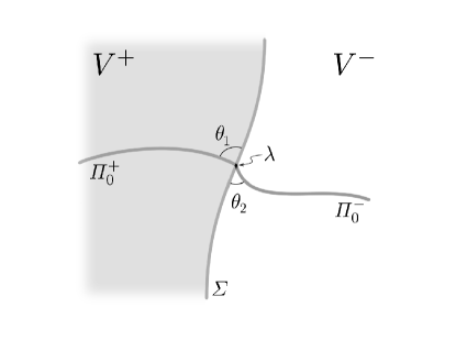
Figure 1: A leaf of the foliation on each side is singled out, $\Pi_{0}^{\pm}$. The intersection of $\Pi_{0}^{\pm}$ with $\Sigma$ is the what we refer to as the corner, $\Lambda$, which is itself a two-surface.

$\Pi^{\pm}_{0}$ are spatial three-surfaces in $V^{\pm}$. We wish to match $\Pi^{-}_{0}$ with $\Pi^{+}_{0}$ across the surface $\Sigma$. However, $\Sigma$ is a timelike three-surface and the intersection of $\Pi^{\pm}$ with $\Sigma$ is a spatial two-surface. Let us call this two-surface the “corner” and denote it by $\Lambda$ with the coordinates $\zeta^{A}$. There is also a two-dimensional space of normals to $\Lambda$. Let $m^{A}_{\alpha}$ be an orthonormal basis for this space.

Fortunately the matching conditions at a corner have already been thoroughly investigated by Taylor [13]. If the Darmois matching conditions are satisfied along two intersecting hypersurfaces then certain conditions must be true at the corner. Thus the matching conditions at a corner are derived from the Darmois conditions. We quote the result here.

The first and second fundamental forms on the corner are defined as

$$\hat{\gamma}_{AB}=\frac{\partial x^{\alpha}}{\partial\zeta^{A}}\frac{\partial x^{\beta}}{\partial\zeta^{B}}g_{\alpha\beta},$$ (17)

$$\hat{K}^{C}_{AB}=\frac{\partial x^{\alpha}}{\partial\zeta^{A}}\frac{\partial x^{\beta}}{\partial\zeta^{B}}\nabla_{\alpha}m^{C}_{\beta}.$$ (18)

There is also a torsion vector defined as,

$$\tau_{A}=\frac{\partial x^{\alpha}}{\partial\zeta^{A}}m^{1\beta}\nabla_{\alpha}m^{2}_{\beta}.$$ (19)

Finally, let $\theta_{A}^{\pm}$ denote the angle between $\Pi^{\pm}$ and $\Sigma$.

Then the two three-spaces $\Pi^{-}$ and $\Pi^{+}$ match at the corner $\Lambda$ if

$$\hat{\gamma}^{-}_{AB}=\hat{\gamma}^{+}_{AB},$$ (20)

$$\hat{K}^{C-}_{AB}=\hat{K}^{C+}_{AB},$$ (21)

$$\tau^{-}_{A}=\tau^{+}_{A}$$ (22)

and

$$\theta_{A}^{-}=\theta_{A}^{+},$$ (23)

where, as above, the superscripts $-$ and $+$ indicates that the quantity is calculated in $V^{-}$ or $V^{+}$.

3 Singularities in the Cheese Slice Universe

We now turn to an example of a spacetime constructed from a matching of exact solutions that satisfy the Darmois conditions and exhibits the AVTD property in the terms described above. The Cheese Slice universe is constructed by matching together FLRW and Kasner spacetimes along planar surfaces [14]. Note that the matched spacetime does not require any additional stress-energy on the matching surface. Such a spacetime could be used to model large scale inhomogeneities in our universe. The ability to combine FLRW regions with large vacuum regions makes the Cheese Slices a more comprehensive cosmological model than the FLRW on its own.

3.1 The Matchings

The FLRW line element in cylindrical coordinates is given by,

$$ds^{2}_{F}=-dt^{2}+a^{2}(t)\left[\frac{dr^{2}}{1-kr^{2}}+r^{2}d\phi^{2}+(1-kr^{2})dz^{2}\right],$$ (24)

with $k=\{-1,0,1\}$. The Kasner line element is given by,

$$ds^{2}_{K}=-dT^{2}+T^{2p_{1}}dX^{2}+T^{2p_{2}}dY^{2}+T^{2p_{3}}dZ^{2},$$ (25)

with the restrictions

$$p_{1}+p_{2}+p_{3}=1=p_{1}^{2}+p_{2}^{2}+p_{3}^{2}.$$ (26)

If the FLRW spacetime is flat and pressure free ($k=0$,$a(t)=t^{4/3}$) and the Kasner exponents are $p_{1}=p_{2}=\frac{2}{3}$, $p_{3}=-\frac{1}{3}$ then one can show that the first and second fundamental forms, eq. (13) and (14), are identical when calculated on the surface $z=z_{0}$ in the FLRW spacetime and $Z=Z_{0}$ in the Kasner spacetime, where $z_{0}$ and $Z_{0}$ are constants. Thus the Darmois conditions are satisfied and we can match these two spacetimes along this surface to construct the Cheese Slice universe. Note that this matching can be repeated indefinitely and with layers of arbitrary thicknesses. See Figure 2(a).

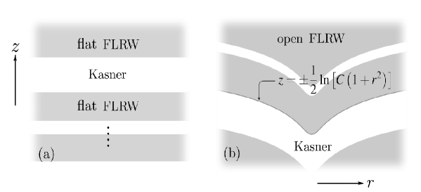
Figure 2: (a) The Cheese slice universe constructed by matching together flat FLRW and Kasner spacetimes along the surface $z=const$. (b) The Cheese Slice universe constructed with open FLRW regions using a different matching surface. Both matchings can be carried on indefinitely with layers of arbitrary thicknesses.

A similar matching can also take place with an open FLRW universe ($k=-1$), but the matching surface must take a different form [15]. In this case the surface must be of the form

$$z=\pm\frac{1}{2}\ln[C(1+r^{2})],$$ (27)

where $C$ is a positive constant. Refer to Figure 2(b) for an illustration of this matching surface.

3.2 The Singularities

Both the Kasner and the FLRW spacetimes have an initial singularities ($t=0=T$). We look at the cases of the flat FLRW matching and the open FLRW matching in turn.

3.2.1 Case (i) Flat FLRW, $k=0$

The coordinates defined in eq. (24) and (25) single out a natural foliation that we will use to check the AVTD property for the flat case. The Kasner spacetimes satisfies the VTD eq. (8)–(11) directly therefore it is trivially AVTD. With the pressure free FLRW spacetime the flat case satisfies the VTD eq. (8)–(11) as well with the following quantities,

$$\tilde{\gamma}_{ab}=a^{2}\,\textrm{diag}\left(1,r^{2},1\right),\qquad\tilde{K}_{ab}=a_{,t}a\,\textrm{diag}\left(1,r^{2},1\right),$$

$$\tilde{\rho}=3\left(\frac{a_{,t}}{a}\right)^{2},\quad\textrm{and}\qquad\tilde{J}_{a}=0=\tilde{S}_{ab},$$ (28)

where $\phantom{a}{}_{,t}=\frac{\partial}{\partial t}$. Thus both sides are AVTD. Furthermore, we can make the coordinate transformation $\tau=-\ln t$ to set the singularity at $\tau=\infty$ and all the conditions of an AVTDS are satisfied.

To show that the matched spacetime is also AVTD with the chosen foliation we must check that the corner conditions, eq. (20)–(23), are satisfied.

On the FLRW side the corner is defined as $z=z_{0}$ and $t=t_{0}$, with $z_{0}$ and $t_{0}$ being constants. Thus we have,

$$\hat{\gamma}^{+}_{AB}=a^{2}\,\textrm{diag}\left(1,r^{2}\right),\qquad\hat{K}^{+1}_{AB}=-a_{,t}a\,\textrm{diag}\left(1,r^{2}\right),$$

$$\hat{K}^{+2}_{AB}=0\qquad\textrm{and}\qquad\tau^{+}_{A}=0.$$ (29)

On the Kasner side the corner is defined as $Z=Z_{0}$ and $T=T_{0}$, with $Z_{0}$ and $T_{0}$ being constants. Thus we have,

$$\hat{\gamma}^{-}_{AB}=\textrm{diag}\left(T^{2p_{1}},T^{2p_{2}}\right),\qquad\hat{K}^{-1}_{AB}=T^{-1}\,\textrm{diag}\left(-p_{1}T^{2p_{1}},-p_{2}T^{2p_{2}}\right),$$

$$\hat{K}^{-2}_{AB}=0\qquad\textrm{and}\qquad\tau^{-}_{A}=0.$$ (30)

If we choose the coordinates on the corner as $\zeta^{A}=\{u,v\}$, parametrize the surface as $r\cos\phi=u=X$ and $r\sin\phi=v=Y$ we can satisfy eq. (20)–(22). Recall that $a=t^{2/3}$ and $p_{1}=p_{2}=2/3$. Furthermore the surfaces defining the corners are orthogonal on both sides and the matching surface subtends an angle of $\pi$ as seen from either side and thus eq. (23) is also satisfied. Therefore we have a matching at the corner and the flat Cheese Slice universe is AVTD.

Also, notice that for the matching to take place we have also identified the time coordinates $t=T$. With the coordinate transformation $\tau=-\ln t=-\ln T$ we can set the singularity at $\tau=\infty$ and the conditions for an AVTDS are satisfied.

3.2.2 Case (ii) Open FLRW, $k=-1$

In general the AVTD property is highly dependent on the choice of foliation. A spacetime that is AVTD in one foliation might not appear to be AVTD in another, thus we must be careful in our choice of foliation. To show that the open Cheese Slices can be AVTD we make the following transformation on the FLRW side,

$$\tilde{z}=z-\frac{1}{2}\ln(1+r^{2}).$$ (31)

The FLRW metric (24) then becomes,

$$ds^{2}_{F}=-dt^{2}+a^{2}(t)\left[dr^{2}+r^{2}d\phi^{2}+2rdrd\tilde{z}+(1+r^{2})d\tilde{z}^{2}\right].$$ (32)

On the Kasner side we will make the transformations,

$$R=\sqrt{X^{2}+Y^{2}},$$ (33)

$$\Phi=\arctan(Y/X),$$ (34)

$$\tilde{Z}=Z-\frac{9}{16b^{5}}\left[-3bT^{\frac{1}{3}}\sqrt{1+b^{2}T^{\frac{2}{3}}}+2b^{3}T\sqrt{1+b^{2}T^{\frac{2}{3}}}+3\ln\left(\sqrt{1+b^{2}T^{\frac{2}{3}}}+bT^{\frac{1}{3}}\right)\right]$$ (35)

and

$$\tilde{t}=\frac{3}{2b^{3}}\left[bT^{\frac{1}{3}}\sqrt{1+b^{2}T^{\frac{2}{3}}}-\ln\left(\sqrt{1+b^{2}T^{\frac{2}{3}}}+bT^{\frac{1}{3}}\right)\right],$$ (36)

where $b$ is a positive constant. With these transformations the Kasner metric (25) becomes,

$$ds^{2}_{K}=-d\tilde{t}^{2}+T^{\frac{4}{3}}\left(dR^{2}+R^{2}d\Phi^{2}\right)+2bd\tilde{t}d\tilde{Z}+T^{-\frac{2}{3}}d\tilde{Z}^{2}.$$ (37)

The matching now takes place along the surface $\tilde{z}=\tilde{z}_{0}$ on the FLRW side and $\tilde{Z}=\tilde{Z}_{0}$ on the Kasner side, with $\tilde{z}_{0}$ and $\tilde{Z}_{0}$ being constants. The coordinates, $\phi=\Phi$ and $t=\tilde{t}$, can be identified along the matching surface. We must also have $r=\frac{2}{3}bR$ and $a^{2}(t)=\frac{9}{4b^{2}}T^{\frac{4}{3}}(\tilde{t})$.

We will use this new foliation to check the AVTD property. Starting with the FLRW case it is straightforward to check that eq. (4)–(7) are satisfied with the following quantities,

$$\begin{array}[]{l}\gamma_{11}=a^{2},\\ \gamma_{13}=a^{2}r,\\ \gamma_{22}=a^{2}r^{2},\\ \gamma_{33}=a^{2}(r^{2}+1),\end{array}\qquad\begin{array}[]{l}K_{11}=a_{,t}a,\\ K_{13}=a_{,t}ar,\\ K_{22}=a_{,t}ar^{2},\\ K_{33}=a_{,t}a(r^{2}+1),\end{array}$$

$$\rho=3\left(\frac{a_{,t}^{2}-1}{a^{2}}\right),\quad\textrm{and}\qquad J_{a}=0=S_{ab}.$$ (38)

The corresponding VTD solution is the flat FLRW solution. We can see that eq. (12) is satisfied and thus the open FLRW is AVTD.

Turning to the Kasner case we find that it also satisfies the VTD eq. (8)–(11) with the lapse and shift being,

$$N=\sqrt{1+b^{2}T^{\frac{2}{3}}}\qquad\textrm{and}\qquad M_{a}=(0,0,b)$$ (39)

respectively. Therefore it is once again trivially AVTD.

Next we check the corner conditions, eq. (20)–(23). The corners on the FLRW and Kasner sides are defined as $\{\tilde{z}=\tilde{z}_{0},t=t_{0}\}$ and $\{\tilde{Z}=\tilde{Z}_{0},\tilde{t}=\tilde{t}_{0}\}$ respectively with $t_{0}$ and $\tilde{t}_{0}$ being constants. Recall that the coordinates are such that $r=\frac{2}{3}bR$ and $\Phi=\phi$. Let us use the superscripts $-$ to denote the Kasner side and $+$ to denote the FLRW side. The first corner condition, eq. (20), is satisfied with,

$$\hat{\gamma}^{-}_{AB}=\textrm{diag}(\frac{9}{4b^{2}}T_{0}^{\frac{4}{3}},RT_{0}^{\frac{4}{3}})=\textrm{diag}(a_{0}^{2},ra_{0}^{2})=\hat{\gamma}^{+}_{AB},$$ (40)

where $T_{0}=T(\tilde{t}_{0})$ and $a_{0}=a(t_{0})$. Let an orthonormal basis of the corner be chosen on both sides such that,

$$\begin{array}[]{ll}m^{-1}_{\alpha}=(0,0,0,T_{0}^{-\frac{1}{3}}\sqrt{1+b^{2}T_{0}^{\frac{2}{3}}})&m^{+1}_{\alpha}=(0,0,0,a_{0})\\ m^{-2}_{\alpha}=(1,0,0,-b)&m^{+2}_{\alpha}=(1,0,0,0)\end{array}.$$ (41)

Then the second corner condition, eq. (21), is satisfied with,

$$\hat{K}^{-1}_{AB}=\frac{3}{2}bT_{0}^{\frac{2}{3}}\,\textrm{diag}(1,\frac{4}{9}b^{2}R^{2})=a_{0}\,\textrm{diag}(1,r^{2})=\hat{K}^{+1}_{AB}$$ (42)

and

$$\hat{K}^{-2}_{AB}=\frac{2}{3b^{2}}T_{0}^{\frac{1}{3}}\sqrt{1+b^{2}T_{0}^{\frac{2}{3}}}\,\textrm{diag}(1,\frac{4}{9}b^{2}R^{2})=a_{,t0}a_{0}\,\textrm{diag}(1,r^{2})=\hat{K}^{+2}_{AB}.$$ (43)

The torsion is identically zero on both sides satisfying eq. (22). On the FLRW side the foliation is orthogonal to the matching surface and the matching surface itself subtends an angle of $\pi$ about the corner. On the Kasner side, the foliation is not orthogonal to the matching surface. Fortunately the matching surface also subtends an angle of $\pi$ about the corner. This ensures condition eq. (23) is satisfied on both sides.

Similar to the flat matching, the time coordinate may be transformed as desired, since it is identical on both sides, to ensure that the singularity is reached as $t\rightarrow\infty$ and the singularity may be considered an AVTDS.

Finally, let us illustrate how this singularity in the Cheese Slice universe manifests itself. In the Kasner regions the initial singularity is of a cigar type and at late times the Kasner regions have pancake-like singularities. In the FLRW slices we have an initial point-like singularity and no singularities at late times. Thus we can visualize the initial singularity of the Cheese Slices as an inhomogeneous chain of cigar-like singularities joined by point-like singularities. At late times, the Cheese Slices become an inhomogeneous matter filled space with pancake-like singularities throughout, as illustrated in Figure (3).

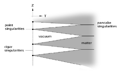
Figure 3: The Singularities of the Cheese Slice Model. The initial singularity is a chain of cigar singularities, corresponding to the Kasner vacuum regions, and point singularities, corresponding to FLRW regions. At late time, the vacuum regions become arbitrarily thin pancake-like singularities.

4 Conclusions

We have proposed a criterion with which we may consider a matched spacetime to be AVTD. First, both sides of the matched spacetime must be AVTD. Secondly each leaf of the chosen foliation must also match across the surface at an intersection that we refer to as the corner. We have also demonstrated this with the example of the Cheese Slice universe. The flat Cheese Slice satisfies these conditions in a straightforward manner whereas the open Cheese slice required more effort to find a foliation that satisfied the AVTD property and the matching conditions. In a general matching it may be difficult to find a foliation that is consistent with the matching and the AVTD property. However, as we have shown, it is possible in the case of Cheese Slice universe for the singularity to inherit the AVTD property from the different spacetimes used in its construction.

In addition to modeling inhomogeneities, these models of matched spacetimes are also very useful in investigating what matching conditions could tell us about the properties of spacetimes themselves. For example, we conjecture that any spacetime that can be smoothly matched to an AVTD spacetime, using the Darmois conditions, must necessarily be AVTD. The resulting matched spacetime would also be AVTD. The general proof of this remains to be seen and is open to investigation. If true, this could lead the way to using the Darmois conditions to prove AVTD properties of other spacetimes.

References

- [1]
- [2] A. Friedmann, Z. Phys. 10 (1922) 377
- [3] G. Lemaître, Annales Soc. Sci. Brux. Ser. I Sci. Math. Astron. Phys. A53 (1933) 51–85
- [4] H. P. Robertson, Astrophys. J. 82 (1935) 284
- [5] A. G. Walker, proc. London math. Soc. 42(90) (1936)
- [6] A. Einstein and E. G. Straus, Reviews of Modern Physics 17 (1945) 120–124
- [7] E. Kasner, American Journal of Mathematics 43(4), (1921) 217–221
- [8] T. J. Broadhurst, R. S. Ellis, D. C. Koo and A. S. Szalay, Nature 343 (1990) 726–728
- [9] V. Belinskii, E. Lifshitz and I. Khalatnikov, Adv. Phys. 19 (1970) 525–573
- [10] D. Eardley, E. Liang and R. Sachs, J. Math. Phys. 13(1) (1972) 99–107
- [11] J. Isenberg and V. Moncrief, Annals of Physics 199 (1990) 84–122
- [12] G. Darmois, Mémorial des Sciences Mathematiques 25 (1927) 25
- [13] J. P. W. Taylor, Class. Quantum Grav. 21 (2004) 3705–3715
- [14] C. C. Dyer, S. Landry and E. B. Shaver, Physical Review D 47(4) (1993) 1404–1406
- [15] C. C. Dyer and C. Oliwa, Class. Quantum Grav. 18 (2001) 2719–2729