Scattering a pulse from a chaotic cavity: Transitioning from algebraic to exponential decay

Abstract

The ensemble averaged power scattered in and out of lossless chaotic cavities decays as a power law in time for large times. In the case of a pulse with a finite duration, the power scattered from a single realization of a cavity closely tracks the power law ensemble decay initially, but eventually transitions to an exponential decay. In this paper, we explore the nature of this transition in the case of coupling to a single port. We find that for a given pulse shape, the properties of the transition are universal if time is properly normalized. We define the crossover time to be the time at which the deviations from the mean of the reflected power in individual realizations become comparable to the mean reflected power. We demonstrate numerically that, for randomly chosen cavity realizations and given pulse shapes, the probability distribution function of reflected power depends only on time, normalized to this crossover time.

I Introduction

Waves and wave behavior are ubiquitous. Examples are acoustic waves in matter, electromagnetic waves, and physical particles in the quantum mechanical regime. Thus understanding wave behavior is important in many different fields; systems which are radically different physically can often be represented by the same mathematics. The simplest model of wave behavior is the Helmholtz equation,

$$(\nabla^{2}+k^{2})\phi=0,$$ (1)

which typically must be supplemented with boundary conditions. Equation (1) describes many physical situations exactly (such as acoustic waves within a homogeneous, linear, bulk medium or quantum particles in free space). Inhomogeneous situations con often be modelled by Eq. (1) with $k\rightarrow k(\vec{r})$ where $k(\vec{r})$ is a function of position. If the system has loss or gain, $k$ can be allowed to become complex. Driving terms can be added to represent transducers or ports. In this paper, we focus on scalar waves described by Eq. (1) with constant $k$, but the results generalize well to many other wave problems.

Unfortunately, for all but the simplest of geometries, Eq. (1) is analytically intractable. Thus techniques, both numerical and theoretical, have been developed to solve Eq. (1). These techniques and their effectiveness vary depending on the regime and physical scenario one wishes to study. In this paper, we limit ourself to the semiclassical regime; i.e., the regime in which the wavelength of the waves excited in the system is much shorter than the scattering elements in the system. In this limit, it is known (via the correspondence principle from Quantum Mechanics) that the resulting dynamics are closely related to the trajectories a classical particle would take through the system. This analogy applies even to purely classical waves, such as waves on the surface of water where the role of classical particle dynamics is now replaced by the dynamical evolution of ray trajectories. In this paper, we consider only those systems in which the corresponding classical dynamics is purely chaotic (i.e., all classical trajectories which start infinitesimally far apart diverge exponentially in time). In addition, we focus on the scattering properties of such systems, assuming that the system of interest is a closed cavity that couples to the outside world only via well-defined localized channels.

The scattering properties of such wave systems have been well studied, both experimentally Weaver (1989); Ellegaard et al. (1995); Chinnery and Humphrey (1996); Chinnery et al. (1997); Lindelof et al. (1986); Blumel et al. (1992) and theoretically Porter (1965); Alhassid (2000); Guhr et al. (1998); Dittes et al. (1992); Alt et al. (1995); Zozoulenko and Blomquist (2003); Buttiker (2000), in a wide variety of contexts. Much of the the theory has focused on the frequency domain, and sophisticated techniques exist to analyze and characterize the scattering process. See Refs. Alhassid (2000) and Guhr et al. (1998); Dittes et al. (1992); Alt et al. (1995); Zozoulenko and Blomquist (2003); Buttiker (2000) and the references cited therein. Similarly, the time domain response of typical wave systems to a delta-function impulse has also been considered Dittes et al. (1992); Alt et al. (1995); Zozoulenko and Blomquist (2003); Buttiker (2000), especially in relationship to fidelity decay(for an overview of fidelity decay, see the Ref. Gorin et al. (2006) and the references therein). In this paper we consider an intermediate situation: we excite the wave system, through an external port with a pulse modulated sinusoidal signal, exciting a large but finite number of modes. The problem of scattering pulse-modulated sinusoidal waves arises in a host of diagnostic situations, such as radar, sonar, nuclear scattering, etc. In what follows, for specificity, we discuss our problem in the context of electromagnetic waves. For simplicity, we consider only lossless two-dimensional microwave cavities excited through a small antenna. We emphasize that the results we obtain can be generalized to higher-dimensional systems and to quantum mechanical or other wave-chaotic systems(e.g., acoustic or elastic wave systems).

On a formal level, the time domain dynamics of such a system is straightforward. The system is open and linear. An incident pulse with a small but finite width in the time domain excites a large number of modes in the cavity, which then radiate their energy back out through the port. Because the system is linear, the reflected voltage can be expressed as a superposition of contributions from modes of the open system. The chaotic dynamics is expressed, not through the dynamics of the individual modes, but rather in the eigenvalue statistics Gutzwiller (1990) and the statistics of the coupling between the port and the cavity.

As showed in Sec. II, the contribution from each mode decays exponentially in time. For short times compared with the Heisenberg time (the inverse of the mean spacing of mode frequencies), the resulting dynamics will be determined primarily by the semiclassical dynamics within the cavity Schomerus and Tworzydlo (2004). However, for large times compared with the Heisenberg time, the ensemble average of the reflected power decreases as a power law in time Dittes et al. (1992). This is due to the fact that there is a probability distribution of mode decay rates which extends to zero decay rate, and for long times the average is dominated by modes with very small decay rates. In the case of a single realization of the chaotic cavity, the incident pulse excites a large number of modes with very similar amplitudes, and consequently the reflected power initially behaves as though the sum of modes were an ensemble average, and the total power decays as a power law. We call this behavior self-averaging. In a single specific realization, however, there are only a finite number of modes excited. Eventually the slowest-decaying mode in the realization will be much larger than the other modes, and the sum will be dominated by this slowest mode, which decays exponentially. Thus for extremely long times we expect that the reflected power for any single realization will fall exponentially, eventually becoming much smaller than the ensemble average.

To test this hypothesis, we have created a program that models the time-domain behavior of generic chaotic systems. It does this by first generating the spectrum and coupling constants of a cavity using the previously published Zheng et al. (2006a) Random Coupling Model (RCM) and then integrating the evolution equations for fields in the cavity, which are modelled in the RCM as a set of driven, damped coupled harmonic oscillators. Single realizations of the power reflected from these cavities, as well as the ensemble average of 50 different cavities, are shown in Fig. 1, where we show two very different realizations: one (Fig. 1(a)) in which the self-averaging persists throughout the length of the time shown and one (Fig. 1(b)) in which self-averaging occurs early, but becomes dominated by solitary slowly decaying modes before the conclusion of the numerical simulation.

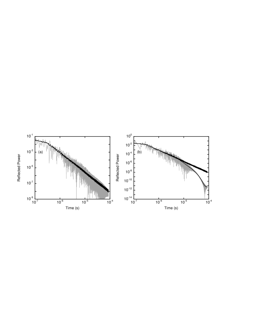
Figure 1: Using the Random Coupling Model (RCM), we created a program capable of simulating the time-domain response of an individual chaotic cavity to a pulse injected into the cavity through a small antenna. By repeatedly creating individual cavities using the RCM, we created an ensemble of such cavities. The gray lines represent the power reflected back into the cavity from two single realizations of the chaotic cavity. The dark solid line represents the reflected power averaged over 50 realizations of the chaotic cavity. The dashed line represents the time-averaged power for the single realization. Figure (a) represents a cavity where self-averaging persists throughout the entire simulation, but figure (b) is dominated by solitary modes after about $10^{-5}$ seconds.

Our goal in this paper is to quantitatively describe the transition from self-averaging to exponential decay. In particular, we wish to predict the time-scale needed to see this transition. In Sec. II, we describe the time-domain model we use for our analysis. In Sec. III, we find the probability distribution function of the decay rates of the open-cavity modes (for the slowest decaying modes in the cavity) as a function of the cavity’s port reflection coefficient. In Sec. IV we find the average, standard deviation and (indirectly) the higher-order moments of the reflected power as a function of time, and use these moments to derive a normalized time which, along with the power spectrum of the incident pulse, is all that is needed to obtain a characterization of the transition from self-averaging to exponential decay. In Sec. V, we evaluate the theory from Sec. IV by numerically finding the number of modes which fall below certain fractions of the average, and we compare the theory with simulation results.

II Model

We base our model system on that used in previous work Zheng et al. (2006a); specifically a quasi-two-dimensional, electromagnetic cavity defined by two conducting plates of area $A$ separated by a distance $h$ which are electrically connected along their perimeters by a conducting side-wall. The cavity is excited by an antenna that induces currents in the plates. The wave equation for this system is

$$\frac{1}{c^{2}}\frac{\partial^{2}}{\partial t^{2}}V_{T}-\nabla^{2}V_{T}=h\mu u\frac{\partial I}{\partial t},$$ (2)

where $c=(\epsilon\mu)^{-1/2}$ is the speed of propagation of waves in the uniform medium inside the cavity, $\epsilon$ and $\mu$ are the permittivity and permeability of this (non-dispersive) medium, $V_{T}(x,y)$ is the voltage difference between the plates, an antenna is modelled through the function $u(x,y)$ which gives the profile of current flowing in the antenna between the surfaces ($\int\int dx\,dy\,u(x,y)=1$), and $I(t)$ is the time-dependent current driving the antenna. Further, as the side walls of the cavity are conducting, $V_{T}=0$ along the perimeter of the cavity. A voltage $V(t)$ is induced at the terminals of the model antenna which is given in terms of the antenna profile $u$ and $V_{T}$

$$V=\int dx\,dy\,uV_{T}.$$ (3)

The antenna is excited by an incident voltage pulse $V_{\textrm{inc}}(t)$ arriving along a transmission line of characteristic impedance $Z_{0}$. The incident wave excites the cavity and produces a reflected wave pulse $V_{\textrm{ref}}(t)$ travelling away from the cavity in the transmission line. At the junction between the transmission line and the cavity the voltages and currents at the antenna and on the transmission line match,

$$V(t) = V_{\textrm{inc}}(t)+V_{\textrm{ref}}(t),$$ (4)

$$I(t) = Z_{0}^{-1}[V_{\textrm{inc}}(t)-V_{\textrm{ref}}(t)].$$ (5)

We now introduce Fourier transforms with transform frequency $\omega$ such that each time-dependent variable is represented in the following way,

$$V_{T}(x,y,t)=\int\frac{d\omega}{2\pi}e^{j\omega t}\bar{V}_{T}(x,y,\omega).$$ (6)

The transformed field within the cavity is then represented as a superposition of the orthonormal modes of the closed cavity,

$$\bar{V}_{T}(x,y,\omega)=\sum_{n}c_{n}(\omega)\phi_{n}(x,y).$$ (7)

where $(\nabla_{x,y}^{2}+k_{n}^{2})\phi_{n}=0$, and $\phi_{n}=0$ on the cavity side walls.

Solving the transformed wave equation gives the amplitudes $c_{n}(\omega)$ which can then be inserted in Eq. (3) to find the transformed voltage,

$$\bar{V}(\omega)=\bar{I}(\omega)Z_{e}(\omega),$$ (8)

where

$$Z_{e}(\omega)=-j\sqrt{\frac{\mu}{\epsilon}}\sum_{n}\frac{kh}{k^{2}-k_{n}^{2}}\left[\int dx\,dy\,u\phi_{n}\right]^{2}$$ (9)

is the (exact) cavity impedance. Here $k_{n}^{2}$ are the eigenvalues of the closed cavity and $k=\omega/c$.

In Ref. (Zheng et al., 2006a, Eq. 14), it was shown that, if one assumed for the purpose of evaluating Eq. (9) that the eigenfunctions behave as if they were a superposition of random plane waves, the overlap between the eigenfunctions and antenna current profile could be expressed in terms of the radiation resistance of the antenna,

$$R_{rad}(k)=\frac{kh}{4}\sqrt{\frac{\mu}{\epsilon}}\int\frac{d\theta}{2\pi}|\bar{u}(\vec{k})|^{2},$$ (10)

where $\bar{u}(\vec{k})$ is the spatial Fourier transform of the profile function $u(x,y)$, and the integral is over the angle $\theta$ of the vector $\vec{k}$.

Here $R_{Rad}=\textrm{Re}[Z_{Rad}]$ where $Z_{Rad}$, the radiation impedance, is the impedance $\bar{V}(\omega)/\bar{I}(\omega)$ that would apply if the cavity side walls were moved to infinity and outward propagating radiation conditions were imposed.

With this random plane wave assumption, the exact impedance $Z_{e}$ in Eq. (9) was replaced by a statistical model impedance,

$$Z(\omega)=-\frac{j}{\pi}\sum_{n}\frac{k\Delta w_{n}^{2}}{k^{2}-k_{n}^{2}}\frac{R_{Rad}(k_{n})}{k_{n}},$$ (11)

where $w_{n}$ are zero mean, unit variance, independent Gaussian random variables. It was further assumed in Ref. Zheng et al. (2006a) that the eigenvalues $k_{n}^{2}$ have the statistical properties of eigenvalues of a Gaussian Orthogonal Ensemble (GOE) random matrix with mean spacing given by Weyl’s formula,

$$\langle k_{n+1}^{2}-k_{n}^{2}\rangle_{n}\equiv\Delta=4\pi/A.$$ (12)

We now use the relationship (Eq. (8)) between the voltage $\bar{V}(\omega)$ and current $\bar{I}(\omega)$ along with the transformed version of Eqs. (4) and (5) to find the transform of the reflected voltage pulse,

$$\bar{V}_{\textrm{ref}}(\omega)=\rho(\omega)\bar{V}_{\textrm{inc}}(\omega),$$ (13)

where the reflection coefficient $\rho(\omega)$ is given by

$$\rho(\omega)=\frac{Z(\omega)-Z_{0}}{Z(\omega)+Z_{0}}.$$ (14)

Although the derivation above has focused on the electromagnetic case, the expression Eq. (14) describes the reflection of a wide variety of waves when they hit an interface, viz., electromagnetic, acoustic, quantum mechanical, etc. The connection becomes closer when one considers, as we will, incident pulses whose transformed bandwidth $\omega_{B}$ is narrow enough that the radiation resistance and mean frequency spacing can be considered constant over the range of excited frequencies.

The time-dependence of the reflected pulse can be found by using the inverse Fourier transformation,

$$V_{\textrm{ref}}(t)=\int\frac{d\omega}{2\pi}\rho(\omega)\bar{V}_{\textrm{inc}}(\omega)e^{j\omega t}.$$ (15)

The long-term behavior of the reflected pulse is governed by the poles of $\rho(\omega)$ (denoted $\omega_{k}$), which satisfy

$$Z_{0}+Z(\omega_{k})=0.$$ (16)

The complex frequencies $\omega_{k}$ have positive imaginary parts as they correspond to decaying modes. We can approximate the long time dependence of the reflected pulse by pushing the inversion contour in Eq. (15) up into the upper half of the $\omega$-plane and deforming it around each pole

$$V_{\textrm{ref}}(t)=-2j\sum_{k}\frac{Z_{0}}{Z^{\prime}(\omega_{k})}\bar{V}_{\textrm{inc}}(\omega_{k})e^{j\omega_{k}t},$$ (17)

where $Z^{\prime}(\omega_{k})=dZ/d\omega|_{\omega=\omega_{k}}$. Thus, the long time behavior of $V_{\textrm{ref}}(t)$ is determined by the properties of eigenfrequencies $\omega_{k}$ of the open system. These eigenfrequencies have real values whose average spacing is denoted by $\Delta\omega$. In principle, $\Delta\omega$ can vary as a function of mode number. If we assume that the incident pulse has a spectrum centered at a carrier frequency $\omega_{0}$, with a bandwidth $\omega_{B}\ll\omega_{0}$ we can relate $\Delta\omega$ to the mean spacing $\Delta$ of $k_{n}^{2}$ values

$$\Delta\omega=\frac{c^{2}\Delta}{2\omega_{0}}.$$ (18)

The inverse of this quantity can be identified with what is known as the Heisenberg time in the Quantum Chaos community.

Each mode has a decay rate $\gamma_{k}=\textrm{Im}(\omega_{k})$ which varies from mode to mode. We denote the probability density function of these decay rates by $P_{\gamma}(\gamma)$. Considering the number of excited modes to be effectively finite, since each mode decays exponentially, the long time behavior of the reflected signal is dominated by modes with the smallest values of $\gamma_{k}$. From Eq. (16), along with the expression for $Z(\omega)$ in Eq. (11), it can be seen that these weakly coupled modes will have particularly small $w_{n}$ and thus $\textrm{Re}(\omega_{k})\simeq k_{n}c$. Given this observation, we can approximate the complex mode frequencies $\omega_{n}$ by solving for the poles in the weak coupling approximation. Specifically, in Eq. (11), our expression for the impedance, we separate the term with $\omega_{n}\simeq k_{n}c$ from the others,

$$Z(\omega_{n})=jX_{n}-j\frac{R_{Rad}(\omega_{0})\Delta\omega w_{n}^{2}}{\pi(\omega_{n}-k_{n}c)},$$ (19)

where we have changed our indexing labels from $k$ to $n$ (because every $k_{n}$ has a corresponding $\omega_{n}$), and

$$X_{n}=-\frac{1}{\pi}\sum_{n^{\prime}\neq n}\frac{k_{n}w_{n^{\prime}}^{2}\Delta}{k_{n}^{2}-k_{n^{\prime}}^{2}}\frac{R_{Rad}(k_{n^{\prime}})}{k_{n^{\prime}}}.$$ (20)

Thus, we can solve Eq. (16) approximately for the complex mode frequencies,

$$\frac{\omega_{n}-k_{n}c}{\Delta\omega}=jw_{n}^{2}\frac{R_{Rad}}{\pi(Z_{0}+jX_{n})}.$$ (21)

From this we obtain an expression for the decay rate,

$$\gamma_{n}=\Delta\omega w_{n}^{2}\frac{R_{Rad}Z_{0}}{\pi(Z_{0}^{2}+X_{n}^{2})}.$$ (22)

The reactance $X_{n}$, like the impedance $Z$ is a statistical quantity. It has an average value to which all the terms in Eq. (20) contribute, and which can be calculated by replacing the sum by an integral Zheng et al. (2006a),

$$\langle X_{n}\rangle=X_{Rad}=-\frac{1}{\pi}P\left\{\int_{0}^{\infty}dk_{n^{\prime}}^{2}\,\frac{k_{n}}{k_{n^{\prime}}}\frac{R_{Rad}(k_{n^{\prime}})}{k_{n}^{2}-k_{n^{\prime}}^{2}}\right\}.$$ (23)

where the symbol $P$ indicates that principal value definition of the the integral is to be taken. This average value is the radiation reactance of the antenna. The reactance $X_{n}$ has a fluctuating part which scales as the radiation resistance and is due primarily to terms in the sum where $n$ and $n^{\prime}$ are not too different,

$$X_{n}=X_{Rad}+R_{Rad}\xi_{n}.$$ (24)

The quantity $\xi_{n}$ has a universal distribution which we will investigate in depth later.

Using Eqs. (19) and (21) we may evaluate $Z^{\prime}(\omega_{n})$ in the denominator of Eq. (17). The result for the reflected signal is

$$V_{\textrm{ref}}(t)=-2\sum_{n}\frac{Z_{0}R_{Rad}}{(Z_{0}+jX_{n})^{2}}w_{n}^{2}e^{j\omega_{n}t}\Delta\omega\bar{V}_{\textrm{inc}}(\omega_{n}).$$ (25)

Taking the magnitude of this, we obtain the reflected power,

$$P_{\textrm{ref}}(t)=\bar{P}_{\textrm{ref}}(t)+\tilde{P}_{\textrm{ref}}(t),$$ (26)

where

$$\bar{P}_{\textrm{ref}}(t)=\sum_{n}\frac{\left|2\pi\Delta\omega\bar{V}_{\textrm{inc}}(\omega_{n})\right|^{2}}{Z_{0}}\frac{\gamma_{n}^{2}}{\Delta\omega^{2}}e^{-2\gamma_{n}t},$$ (27a)

$$\tilde{P}_{\textrm{ref}}(t)=\sum_{n,m\neq n}\frac{\left|2\pi\Delta\omega\right|^{2}\bar{V}_{\textrm{inc}}(\omega_{n})\bar{V}_{\textrm{inc}}^{*}(\omega_{m})}{Z_{0}}\frac{\gamma_{n}\gamma_{m}}{\Delta\omega^{2}}e^{j(\omega_{n}-\omega_{m}^{*})t}e^{2j(\psi_{m}-\psi_{n})},$$ (27b)

and $\psi_{n}$ is the phase of $Z_{0}+jX_{n}$.

The two contributions to the reflected power (27a) and (27b) are very different. In the first contribution the terms decay exponentially and smoothly and the sum is always positive. In fact, if we smooth over a timescale longer than the Heisenberg time, this first term will remain essentially unchanged. The second term, on the other hand, oscillates rapidly on a timescale comparable to the Heisenberg time, but tends to zero if averaged over long timescales. For the very long timescales needed to see the transition from self-averaging to exponential decay, we can treat the rapidly fluctuating terms in $P_{\textrm{ref}}(t)$ as random variables with the phases in the exponents ($\left(\omega_{n}-\omega_{m}^{*}\right)t$) being uniformly distributed. Under this assumption, we find that, for a single realization of the chaotic cavity, the fluctuating part of $P_{\textrm{ref}}$ is random and has a variance of

$$\sigma^{2}=\langle\left[\tilde{P}_{\textrm{ref}}(t)\right]^{2}\rangle_{t}\leq\bar{P}^{2}_{\textrm{ref}}(t).$$ (28)

where $\langle\ldots\rangle_{t}$ indicates a sliding averaging in $t$ over a timescale that is long compared to the Heisenberg time but short compared to the characteristic time for variation of $\bar{P}_{\textrm{ref}}(t)$. That is, the order of magnitude of the oscillating part of $P_{\textrm{ref}}$ is typically the same as that of the smoothed part. Thus, if the smoothed part of $P_{\textrm{ref}}$ drops exponentially, the fluctuations around it will as well. Hence, if the power stays self-averaged, the fluctuations will be as large as the signal itself. When we consider the transition from self-averaging to exponential decay, we consider only the statistics of the smoothed part of $P_{\textrm{ref}}$, ignoring the oscillating part which does not contribute to the self-averaging. Thus in our theory we consider only the time-averaged power $\bar{P}_{\textrm{ref}}(t)$, Eq. (27a), which is the key result of this section.

III Finding $P_{\gamma}(\gamma_{n})$

From Eq. (27a), we see that the average reflected power is a sum over contributions from exponentially decaying modes. Because of the exponential decay, the relative amplitudes of the modes will separate exponentially in time, with the modes with the smallest $\gamma_{n}$ eventually dominating the sum. Thus, the crossover time from self-averaging to exponential decay depends on the behavior of the probability distribution function of $\gamma_{n}$ for small values of $\gamma_{n}$. In this section we find the behavior of $P_{\gamma}(\gamma_{n})$, the probability distribution function for the decay rates for $\gamma_{n}\ll\Delta\omega$. Previous work has been done on the subject (for instance, in the case of a lasing chaotic cavity, see Refs. Frahm et al. (2000); Schomerus et al. (2000)), including analytical solutions for the $P_{\gamma}(\gamma)$ for all $\gamma$ Fyodorov and Sommers (1997); Sommers et al. (1999), but because we focus on the single port case with time reversal symmetry for small $\gamma$ only, many approximations can be made which greatly simplify the derivation, which we present here.

We start by considering the statistics of $\xi_{n}$, where $\xi_{n}$ is defined in Eq. (24). We show in Appendix A that the statistics of $\xi_{n}$ are given in terms of the angle $\psi_{n}=\tan^{-1}(\xi_{n})$, where $\psi_{n}$ is distributed according to the pdf,

$$P_{\psi_{n}}(\psi_{n})=\frac{\cos(\psi_{n})}{2}.$$ (29)

Using this result and Eq. (22), we find an expression for $P_{\gamma}(\gamma_{n})$ where $\gamma_{n}\ll\Delta\omega$:

$$P_{\gamma}(\gamma_{n})=\frac{1}{\sqrt{2\pi}}\int_{-\pi/2}^{\pi/2}d\psi_{n}\,\cos\psi_{n}\int_{0}^{\infty}dw\,e^{-w^{2}/2}\delta\left(\gamma_{n}-w^{2}\frac{r_{r}\Delta\omega}{\pi\left[1+(r_{r}\tan(\psi_{n})+x_{r,n})^{2}\right]}\right),$$ (30)

where $r_{r}=R_{Rad}(k)/Z_{0}$ and $x_{r}=X_{Rad}(k)/Z_{0}$. The innermost integral can be evaluated leaving only an integral over $\psi_{n}$. Further, since we are only interested in the case of small $\gamma_{n}\ll\Delta\omega$, the main contribution comes from $|w|\ll 1$. The result is

$$P_{\gamma}(\gamma_{n})\cong\frac{P_{0}}{2\sqrt{\gamma_{n}\Delta\omega}}\textrm{ for }\gamma_{n}\ll\Delta\omega,$$ (31)

where

$$P_{0}=(2r_{r})^{-1/2}\int_{-\pi/2}^{\pi/2}d\psi_{n}\,\sqrt{\cos^{2}\psi_{n}+(r_{r}\sin\psi_{n}+x_{r}\cos\psi_{n})^{2}}.$$ (32)

The quantity $P_{0}$ given in Eq. (32) can be rewritten in terms of the radiation reflection coefficient of the port that applies when the walls of the cavity have been moved out to infinity,

$$\rho_{r}=\frac{z_{r}-1}{z_{r}+1},$$ (33)

where $z_{r}=r_{r}+ix_{r}=(R_{Rad}+jX_{Rad})/Z_{0}$ is the normalized radiation impedance of the antenna. To see this, we introduce the intermediate variable $\beta=z_{r}^{2}-1$ and define a new integration variable $\phi=\psi_{n}-\textrm{arg}(\beta)/2$ in Eq. (32). The result of these variable changes is

$$P_{0}=\sqrt{2\frac{1-|\rho_{r}|}{1+|\rho_{r}|}}E\left(\frac{2j\sqrt{|\rho_{r}|}}{1-|\rho_{r}|}\right),$$ (34)

where

$$E(k)=\int_{0}^{\pi/2}d\phi\,\sqrt{1-k^{2}\sin^{2}(\phi)}$$ (35)

is the complete elliptic integral of the second kind.

We confirm Eqs. (31) and (34) numerically by generating an ensemble of $\gamma_{n}$ values. To do this we solve Eq. (16) by generating different realizations of the Gaussian random variables $w_{n}$ and random matrix eigenvalues $k_{n}^{2}$ appearing in the definition of $Z(\omega)$, Eq. (11). We find the mode frequencies by noting that as $Z_{0}\rightarrow\infty$, $\omega_{n}\rightarrow k_{n}c$ for all modes. We then introduce $Y_{0}=Z_{0}^{-1}$ and differentiate both sides of Eq. (16) with respect to $Y_{0}$, obtaining a differential equation for $\omega_{n}(Y_{0})$,

$$\frac{d\omega_{n}}{dY_{0}}=\frac{Z^{2}(\omega_{n})}{Z^{\prime}(\omega_{n})},$$ (36)

which can be solved numerically to find $\omega_{n}$ for finite $Z_{0}$. Note that although both $Z^{2}(\omega_{n})$ and $Z^{\prime}(\omega_{n})$ are singular as $\omega_{n}\rightarrow k_{n}c$, their ratio is finite.

By generating 1000 different realizations of $k_{n}^{2}$ and $\omega_{n}$ (truncating the spectrum to include only 600 terms), and integrating Eq. (36) numerically using fourth-order Runga-Kutta from $Y_{0}=0$ to $Y_{0}=R_{Rad}^{-1}$, it is possible to generate pdfs of $\tilde{w}_{n}\equiv\sqrt{\gamma_{n}}$ as a function of $|\rho_{r}|$. We choose the pdfs of $\tilde{w}_{n}$ instead of $\gamma_{n}$ because $P_{\tilde{w}}(\tilde{w}=0)=P_{0}/\Delta\omega$, which is finite and thus numerically easier to fit. The results are shown in Fig. 2 where the numerical results and the theory are seen to be in clear agreement. We note that this numerical test (solving Eq. (36) for $Y_{0}=R_{Rad}^{-1}$) does not assume the weak coupling limit and thus confirms our assumptions in obtaining Eq. (34).

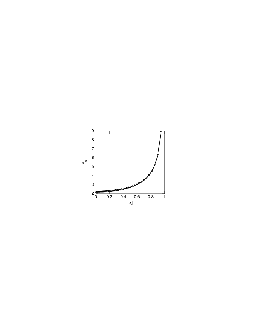
Figure 2: A comparison of numerically generated values for $P_{0}$ (circles) with the theoretical result from Eq. (34) (the solid line). The circles represent numerical calculations of $P_{0}$ with the radiation reactance of the port set to be $X_{Rad}=0$. To get different values of $|\rho_{r}|$, $Y_{0}$ was changed as described in Eq. (36).

IV The Statistics of $\bar{P}_{\textrm{ref}}(t)$

The smoothed reflected power $\bar{P}_{\textrm{ref}}(t)$ given by Eq. (27a) is a sum of terms each of which is a random variable. The terms are not strictly independent. This follow from the fact that there are correlations between the eigenvalues of the closed system, and $\gamma_{n}$, given by Eq. (22), depends on these eigenvalues through the reactance $X_{n}$, defined in Eq. (20). Fortunately the correlation is significant only for almost adjacent modes. For times large enough that the self-averaging breaks, the fraction of modes contributing will be small, and thus, the majority of contributing modes will be well separated and approximately independent of each other.

Hence for our purposes, $\bar{P}_{\textrm{ref}}$ can be treated as a sum of a large number of independent terms. Thus, for times when a large number (but small fraction) of modes have comparable magnitudes, for an ensemble of cavity realizations, $\bar{P}_{\textrm{ref}}$ is a Gaussian random variable centered on $\langle\bar{P}_{\textrm{ref}}(t)\rangle$ with a small standard deviation. As we demonstrate in the following sections, the standard deviation starts out small, but as the number of contributing modes decreases, the standard deviation increases relative to the mean, eventually becoming much larger than the mean. As this happens, the simple Gaussian distribution changes into a more complex distribution with the majority of modes becoming much smaller than the average, corresponding to the shift from self-averaging to exponential decay.

These shifts can be treated analytically by considering the moments of $\bar{P}_{\textrm{ref}}$. We first (Sec.  IV.1) consider the mean and standard deviation of $\bar{P}_{\textrm{ref}}$ to find a scaling law describing the transition from Gaussian to non-Gaussian behavior. Armed with the results from this comparison, in Sec. IV.2 we generalize the results to higher-order moments (via the cumulants), showing that for large times all moments of $\bar{P}_{\textrm{ref}}$ obey the same scaling law. We then numerically demonstrate that the cumulative distribution function of $\bar{P}_{\textrm{ref}}/\langle\bar{P}_{\textrm{ref}}\rangle$ satisfies the scaling law for multiple pulse shapes, as predicted.

IV.1 The Mean and Variance

We can calculate the mean and the variance of $\bar{P}_{\textrm{ref}}$ for all times as

$$\langle\bar{P}_{\textrm{ref}}\rangle=\sum_{n}\frac{|2\pi\Delta\omega\bar{V}_{\textrm{inc}}(\omega_{n})|^{2}}{Z_{0}}\mu_{1},$$ (37)

and

$$\langle(\bar{P}_{\textrm{ref}}-\langle\bar{P}_{\textrm{ref}}\rangle)^{2}\rangle=\sum_{n}\frac{|2\pi\Delta\omega\bar{V}_{\textrm{inc}}(\omega_{n})|^{4}}{Z_{0}^{2}}(\mu_{2}-\mu_{1}^{2}),$$ (38)

where

$$\mu_{m}(t)=\int_{0}^{\infty}\frac{d\gamma P_{0}}{2\sqrt{\gamma\Delta\omega}}\left[\frac{\gamma^{2}}{\Delta\omega^{2}}e^{-\gamma t}\right]^{m}.$$ (39)

Evaluation of the integral in Eq. (39) gives

$$\mu_{m}(t)=\frac{P_{0}}{2(m\Delta\omega t)^{2m+1/2}}\Gamma(2m+1/2).$$ (40)

Equations (37) and (39) give the result that the average reflected power (averaged over an ensemble of reflecting cavities) decreases as a power law in time, which is in agreement with previous theory Dittes et al. (1992); Dittes (2000),

$$\langle\bar{P}_{\textrm{ref}}(t)\rangle\sim t^{-5/2}.$$ (41)

Equation (38) is useful for finding the range of values that are most likely to contain $\bar{P}_{\textrm{ref}}$; for small times with an approximately Gaussian pdf for $\bar{P}_{\textrm{ref}}$, we expect that the majority of realizations will fall within the range $[\langle\bar{P}_{\textrm{ref}}\rangle-2\sigma_{P},\langle\bar{P}_{\textrm{ref}}\rangle+2\sigma_{P}]$ where $\sigma_{P}=\langle(\bar{P}_{\textrm{ref}}-\langle\bar{P}_{\textrm{ref}}\rangle)^{2}\rangle^{1/2}$. For large times, however, $\sigma_{P}>\langle\bar{P}_{\textrm{ref}}\rangle$. We see this by first considering the ratio

$$\frac{\mu_{2}}{\mu_{1}^{2}}=\frac{(\Delta\omega t)^{1/2}}{P_{0}}\frac{\Gamma(9/2)}{2^{7/2}\Gamma(5/2)^{2}}.$$ (42)

Thus, for large times, $\mu_{2}\gg\mu_{1}^{2}$, and $\mu_{2}$ dominates Eq. (38). For large times, we have

$$\frac{\sigma_{P}^{2}}{\langle\bar{P}_{\textrm{ref}}\rangle^{2}}=\frac{(t\Delta\omega)^{1/2}}{P_{0}}\frac{\Gamma(9/2)}{2^{7/2}\Gamma(5/2)^{2}}\frac{\sum_{n}|V_{\textrm{inc}}(\omega_{n})|^{4}}{\left[\sum_{n}|V_{\textrm{inc}}(\omega_{n})|^{2}\right]^{2}}$$ (43)

Equation (43) can be made more transparent by considering the sums over $|V_{\textrm{inc}}|^{2m}$. The incident pulse can be considered to have two independent properties: a shape and a width. If we double the width of the pulse in the frequency domain (or equivalently if we halve the average mode separation) without changing the shape, the sums in Eq. (43) will, to a good approximation, simply double. We thus define the effective number of modes excited by the wave to be

$$N=\frac{\left[\sum_{n}|V_{\textrm{inc}}(\omega_{n})|^{2}\right]^{2}}{\sum_{n}|V_{\textrm{inc}}(\omega_{n})|^{4}}.$$ (44)

In the case of a square wave excitation in the frequency domain, Eq. (44) gives exactly the number of modes excited. In the case of more typical pulses, such as a Gaussian pulse, Eq. (44) defines a relationship between the pulse width and the number of significant excited modes.

Substituting Eq. (44) into Eq. (43), we get

$$\frac{\sigma_{P}^{2}}{\langle\bar{P}_{\textrm{ref}}\rangle^{2}}=\tau^{1/2}\frac{\Gamma(9/2)}{2^{7/2}\Gamma(5/2)^{2}},$$ (45)

where

$$\tau=\frac{t\Delta\omega}{N^{2}P_{0}^{2}}.$$ (46)

As long as $\sigma_{P}/\langle\bar{P}_{\textrm{ref}}\rangle$ is small, it is reasonable to expect the majority of realizations of $\bar{P}_{\textrm{ref}}$ to be within two sigma of the average, and numerically we find that this is true. From Eq. (45), we see that for $t\Delta\omega\gg 1$ and $\tau\ll 1$ (possible because $N$ is assumed to be large) this is possible. Eventually the standard deviation will be comparable to the mean and for very long times the standard deviation will be much larger than the mean. This shift corresponds to the change from self-averaging to exponential decay.

IV.2 Higher Moments

An analysis of the higher moments of $\bar{P}_{\textrm{ref}}$ follows essentially the same steps as those to find the mean and variance. We find the moments of $\bar{P}_{\textrm{ref}}$ by finding the moments of the individual terms in $\bar{P}_{\textrm{ref}}$, dropping all but the leading order term in $t^{-1/2}$, and combining them properly to get the moments of the sum. We cannot do this by simply summing the moments of the individual terms; the sums of the moments are not in general the moments of the sum. However, if we define the moment-generating function,

$$M(h)=\langle e^{h\bar{P}_{\textrm{ref}}}\rangle=1+\sum_{p=1}^{\infty}\frac{h^{p}\langle\bar{P}_{\textrm{ref}}^{p}\rangle}{p!},$$ (47)

we see that the moments of $\bar{P}_{\textrm{ref}}$ are given by

$$\langle\bar{P}_{\textrm{ref}}^{m}\rangle=M^{(m)}(0).$$ (48)

Here $M^{(m)}(h)$ is the $m$th derivative of $M(h)$ with respect to its argument. This can be related to a function known as the cumulant-generating function

$$g(h)=\log(M(h))=\sum_{p=1}^{\infty}\kappa_{p}\frac{h^{p}}{p!}$$ (49)

where $\kappa_{m}$ is the $m$th cumulant, defined as

$$\kappa_{m}=g^{(m)}(0).$$ (50)

We show in Appendix (B) that, in analogy to Eq. (43), the higher-order cumulants (and thus all higher-order moments) of $\bar{P}_{\textrm{ref}}$ are given by

$$\frac{\kappa_{m}}{\kappa_{1}^{m}}=\left(2\sqrt{\tau}\right)^{m-1}\frac{\Gamma(2m+1/2)}{m^{2m+1/2}\Gamma(5/2)^{m}}\frac{N^{m-1}\sum_{n}|V_{\textrm{inc}}(\omega_{n})|^{2m}}{\left(\sum_{n}|V_{\textrm{inc}}(\omega_{n})|^{2}\right)^{m}}.$$ (51)

If we use the definition of $N$ from Eq. (44) and approximate all sums over $n$ with integrals over $\omega_{n}$, we find that the expression $N^{m-1}\sum_{n}|V_{\textrm{inc}}(\omega_{n})|^{2m}/\left(\sum_{n}|V_{\textrm{inc}}(\omega_{n})|^{2}\right)^{m}$ is, to a good approximation, independent of the width of the power spectrum but dependent on the shape. In the case of a square power spectrum, this factor is identically one for all $m$. For a Gaussian pulse we find that

$$\frac{N^{m-1}\sum_{n}|V_{\textrm{inc}}(\omega_{n})|^{2m}}{\left(\sum_{n}|V_{\textrm{inc}}(\omega_{n})|^{2}\right)^{m}}=\sqrt{\frac{2^{m-1}}{m}}.$$ (52)

Similarly, for a pulse with a Lorentzian power spectrum,

$$\frac{N^{m-1}\sum_{n}|V_{\textrm{inc}}(\omega_{n})|^{2m}}{\left(\sum_{n}|V_{\textrm{inc}}(\omega_{n})|^{2}\right)^{m}}=\frac{2^{m-1}\Gamma(m-\frac{1}{2})}{\sqrt{\pi}\Gamma(m)}.$$ (53)

Equation (51), combined with replacing the sums over $|V_{\textrm{inc}}(\omega)|^{2m}$ with integrals, demonstrates the most important theoretical result of this paper: all statistical properties of the reflected power depend only on the shape of the pulse (independent of width) and the normalized time $\tau$ defined in Eq. (46). Thus the cross-over from self-averaging to exponential decay, no matter how measured, will depend only on $\tau$ and the pulse shape.

V Numerical Results

In this section, we compare different methods of calculating $\bar{P}_{\textrm{ref}}(t)$ to show that our theoretical conclusions are correct. To view the resulting distributions, we find the ensemble average of the calculated values of $\bar{P}_{\textrm{ref}}(t)$ and then compare the individual realizations to the average. In particular, we define $C(\alpha,\tau)$ to be the fraction of realizations which are less than $\alpha$ times the ensemble average (i.e. $C(\alpha,\tau)$ is the cumulative distribution of $\bar{P}_{\textrm{ref}}$ at the normalized time $\tau$).

To both test and evaluate the theoretical results in Sec. IV, we perform two separate, independent calculations which should, according to our theory, produce the same results. The first method calculates the sum in Eq. (27a) with the $\gamma_{n}$ independent of $\textrm{Re}(\omega_{n})$ and distributed according to the Porter-Thomas distribution with one degree of freedom,

$$P(\gamma)=\frac{e^{-\gamma/2}}{\sqrt{2\pi\gamma}}.$$ (54)

This distribution is chosen because it has the same behavior for small $\gamma$ as is indicated in Eq. (31). We consider two different pulse spectra, $\bar{V}_{\textrm{inc}}(\omega_{n})$, Gaussian and Lorentzian, with two different widths $N=20$ and $30$, where $N$ is defined in Eq. (44). Finally, we take the $\omega_{n}$ to be uniformly spaced when evaluating the sums. We call these results the theoretical results because they are a numerical evaluation of the theoretical assumptions used in Sec. IV. The theoretical results are shown in Fig. 3 for the case of the two pulse shapes and two spectral widths. The first thing to note about the plots is that the results for $N=20$ and $N=30$ lie on top of each other, showing that the definition of $\tau$(46) correctly accounts for variation of the pulse width. (There is a small deviation in the Lorentzian case for small values of $\alpha$ that will be addressed subsequently.) The second thing to note is that the $C(\alpha>0.3)$ curves for the two pulse shapes are very similar. Thus, the fraction of realizations close to or greater than the mean is the same in the two cases. Where the two pulse shapes differ is for times $\tau\gg 1$ and small $\alpha\ll 1$. In the Gaussian case almost all realizations fall well below the average as $\tau$ gets large, whereas in the Lorentzian case there is a larger fraction of realizations with measurable power ($\alpha>0.001$) at late time. This is due to the long tail in the Lorentzian distribution exciting a large number of modes with small but significant levels of power. The difference between the $N=20$ and $N=30$ cases is due to truncation of the spectrum at $600$ modes.

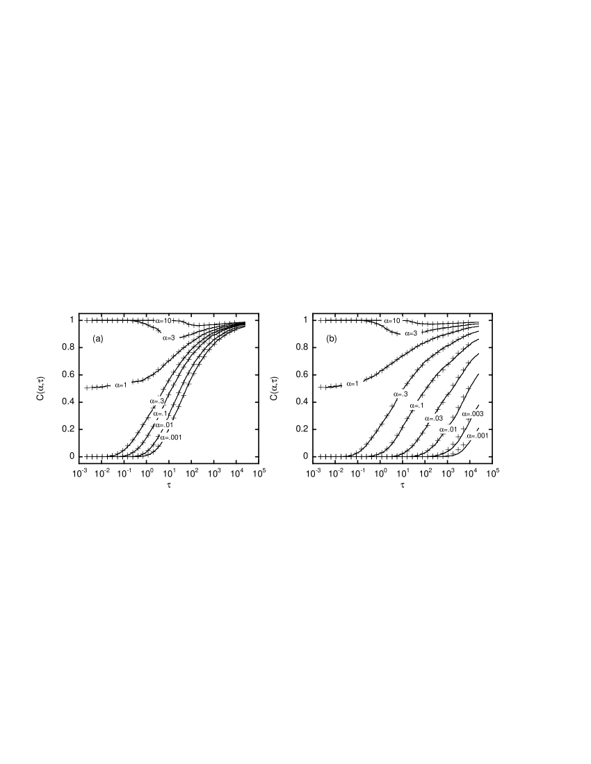
Figure 3: The fraction of realizations of $\bar{P}_{\textrm{ref}}$ which are less than $\alpha\langle\bar{P}_{\textrm{ref}}\rangle$ as a function of normalized time $\tau$ for (a) a Gaussian spectrum and (b) a Lorentzian spectrum. The black lines(‘+’ symbols) represent the statistics for $N=20(30)$. Note that plots for $N=20$ and $N=30$ are slightly different for the Lorentzian case with small $\alpha$. This is due to the fact that the contributions for small $\alpha$ come from the tails of the distribution, which we numerically truncated to calculate these plots.

The second test employs the time-domain code used to generate the data in Fig. 1. We then time-smooth the resulting power (using a Gaussian window with a width of $10$ Heisenberg times) to calculate $\bar{P}_{\textrm{ref}}$. The time domain code is described in Appendix C. In Fig. (4) we compare results for $C(\alpha,\tau)$ using 50 realizations with the theoretical curves. The time-domain code is run only to $\tau=1$ which for these parameters corresponds to $~{}1744$ Heisenberg times. The time domain simulation results agree well with the theoretical results considering the finite sample size.

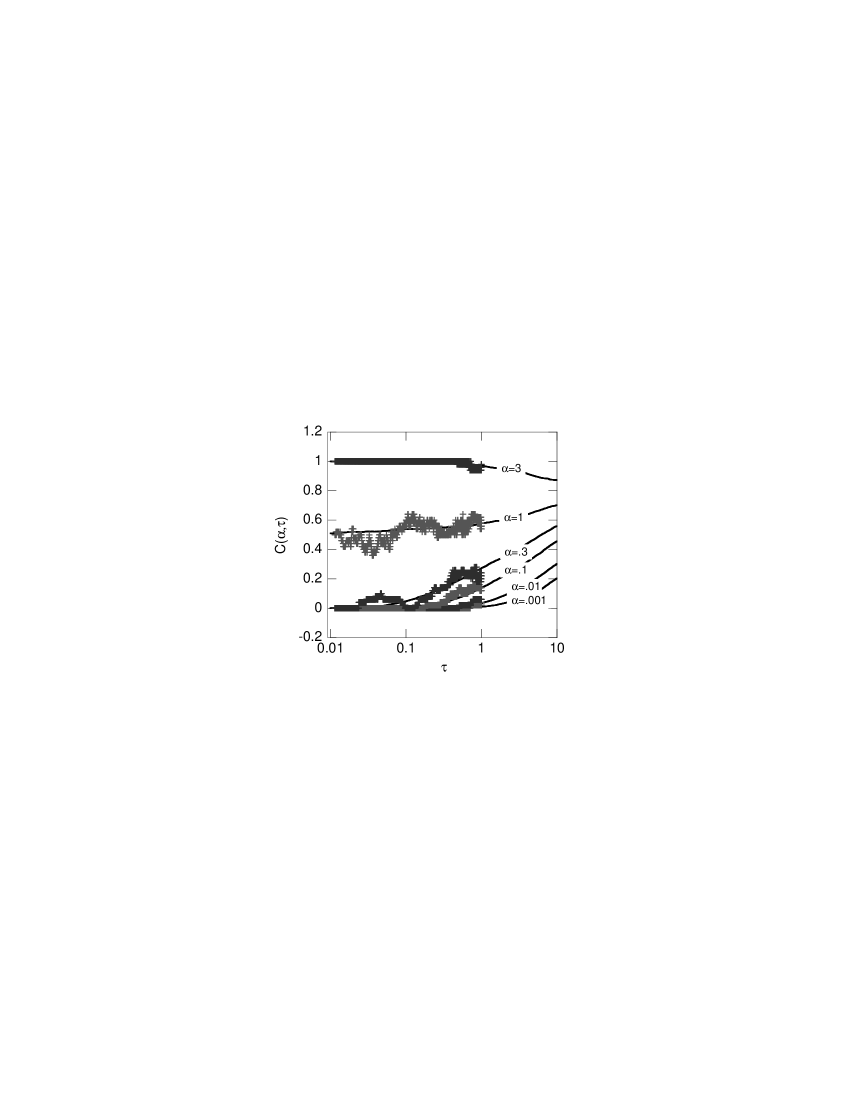
Figure 4: The fraction of realizations of $\bar{P}_{\textrm{ref}}$ which are less than $\alpha\langle\bar{P}_{\textrm{ref}}\rangle$ as a function of normalized time $\tau$ for the theoretical results calculated numerically (the solid lines) and the same results calculated from integrating Eq. (2) directly (indicated by the ‘+’ symbols). Random Matrix Theory is explicitly used to calculate the spectrum and coupling constants for the time-domain integration.

In addition, we have performed tests which have allowed the value of $P_{0}$ to vary, and have solved Eq. (36) to get the complex values of $\omega_{n}$. The results agree well with the theoretical results of Fig. 3 and are not displayed.

VI Conclusions

In this paper, we have found numerically and theoretically that the long term behavior of power reflected from a lossless, microwave cavity excited through a single port self-averages for times larger than the Heisenberg time, decaying as a power law in time. We have also found, theoretically and numerically, that for times much longer than the Heisenberg time, when $\tau$, the normalized time, is of order 1, that single modes in the cavity will begin to dominate the long term decay and the reflected power will begin to decay exponentially. The details of this behavior have been found to depend on the shape of the power spectrum of the incident pulse that excited the cavity, but to otherwise depend only on the normalized time. Because much of the theory used to derive this behavior depends only on generic Random Matrix Theory, we expect that this behavior will translate into other lossless wave-chaotic systems (e.g., acoustic, quantum mechanical, etc.), independent of details.

Appendix A Finding the Distribution of $\xi_{n}$ for Small $\gamma_{n}$

To find the distribution of $\xi_{n}$ defined in Eq. (24) for small $\gamma_{n}$, we exploit the fact that, in a two-port system with the ports identical and described by Random Matrix Theory, the diagonal elements of the normalized impedance matrix each have the same statistics as the single-port normalized impedance. Then using the exact statistics of the two-port RMT impedance, we can find the statistics of the one-port impedance (20).

We see this by first writing the elements of the two-port normalized impedance matrix as a sum, analogous to Eq. (11),

$$\xi_{i,j}=-\frac{j}{\pi}\sum_{n}\frac{w_{i,n}w_{j,n}}{k^{2}-k_{n}^{2}},$$ (55)

where the $w_{i,n}$ are independent Gaussian random variables and the $k_{n}^{2}$ have the statistics of the eigenvalues of a GOE random matrix.

As shown in previous work Zheng et al. (2006b), the 2x2 matrix $\xi$ has the following statistics: its eigenvalues $\tan\theta_{1}$, and $\tan\theta_{2}$ have a joint pdf,

$$P(\theta_{1},\theta_{2})\propto\left|\sin\left(\frac{\theta_{2}-\theta_{1}}{2}\right)\right|,$$ (56)

and its eigenvectors $(\cos\nu,\sin\nu)$ and $(-\sin\nu,\cos\nu)$ have $\nu$ uniformly distributed and independent of $\theta_{1}$ and $\theta_{2}$. Consequently, a diagonal element of $\xi$ can also be parameterized as

$$\xi_{i,i}=\cos^{2}\eta\tan\theta_{1}+sin^{2}\eta\tan\theta_{2}.$$ (57)

Comparing Eqs. (55) and (57), we see that the singularity at $k=k_{n}$ in Eq. (55) is matched by either $\theta_{1}$ or $\theta_{2}$ going through $\pi/2$; for specificity we assume that it is $\theta_{1}$. For small $\gamma_{n}$, corresponding to small $w_{n}^{2}$, the coefficient of the singularity is small, which corresponds to $\cos^{2}\eta\approx 0$. Thus, for small $\gamma_{n}$, $\xi_{n}$ has the statistics given by

$$\xi_{n}=\tan\theta_{2}|_{\theta_{1}=\pi/2}$$ (58)

which inserted into Eq. (56) produces the pdf for $\psi_{n}=\tan^{-1}\xi_{n}=\theta_{2}$

$$P(\psi_{n})=\frac{\cos\psi_{n}}{2}$$ (59)

Numerically we confirm this by generating a single 600x600 element matrix from the Gaussian Orthogonal Ensemble and calculating and scaling the eigenvalues to get an appropriate spectrum. We then repeatedly generate 600 realizations of 600 coupling constants and use them to calculate 360,000 realizations of $X_{n}$, which we then normalize to calculate $\psi_{n}$. The resulting statistics are demonstrated in Fig. 5.

Figure 5: A comparison of a numerically-generated pdf of $\psi_{n}$ (‘+’ symbols) with the anticipated result from Eq. (59), $\cos(\psi_{n})/2$ (the solid line).

Appendix B Finding the Cumulants of $\bar{P}_{\textrm{ref}}$

To obtain Eq. (51), we note that the cumulant generating function of $\bar{P}_{\textrm{ref}}$ obeys

$$g(h) = \log\left(\left\langle\exp\left(h\sum_{n}\frac{\left|2\pi\Delta\omega\bar{V}_{\textrm{inc}}(\omega_{n})\right|^{2}}{Z_{0}}\frac{\gamma_{n}^{2}}{\Delta\omega^{2}}e^{-2\gamma_{n}t}\right)\right\rangle\right)$$ (60)

$$= \sum_{n}\log\left(\left\langle\exp\left(h\frac{\left|2\pi\Delta\omega\bar{V}_{\textrm{inc}}(\omega_{n})\right|^{2}}{Z_{0}}\frac{\gamma_{n}^{2}}{\Delta\omega^{2}}e^{-2\gamma_{n}t}\right)\right\rangle\right).$$

This result is a specific example of a general property of cumulants Kenney and Keeping (1951): The $m$th cumulant of a sum of independent variables is the sum of the $m$th cumulants of the single variables. Thus, in analogy to Eq. (49), we define the cumulant-generating function and the cumulants $\tilde{\kappa}_{p}$ for each term in the sum in Eq. (60) as

$$\tilde{g}(q)=\log\left(\left\langle\exp\left(q\frac{\gamma_{n}^{2}}{\Delta\omega^{2}}e^{-2\gamma_{n}t}\right)\right\rangle\right)=\sum_{p=1}^{\infty}\tilde{\kappa}_{p}\frac{q^{p}}{p!},$$ (61)

and by matching coefficients of $h^{m}$ in Eq. (60), we get that

$$\kappa_{m}=\tilde{\kappa}_{m}\sum_{n}\frac{\left|2\pi\Delta\omega\bar{V}_{\textrm{inc}}(\omega_{n})\right|^{2m}}{Z_{0}^{m}}.$$ (62)

All that is left is to find the long-term behavior for $\tilde{\kappa}_{m}$. To do this, we note that we can rewrite the average exponential in Eq. (61) as

$$\left\langle\exp\left(q\frac{\gamma_{n}^{2}}{\Delta\omega^{2}}e^{-2\gamma_{n}t}\right)\right\rangle=1+\sum_{n=1}^{\infty}\frac{q^{n}\mu_{n}}{n!}.$$ (63)

Because $q$ is a dummy variable which can be arbitrarily small, we can also expand the logarithm in Eq. (61) to get that

$$\sum_{p=1}^{\infty}\tilde{\kappa}_{p}\frac{q^{p}}{p!}=\sum_{n=1}^{\infty}\frac{q^{n}\mu_{n}}{n!}-\frac{1}{2}\left(\sum_{n=1}^{\infty}\frac{q^{n}\mu_{n}}{n!}\right)^{2}+\frac{1}{3}\left(\sum_{n=1}^{\infty}\frac{q^{n}\mu_{n}}{n!}\right)^{3}-\ldots.$$ (64)

By matching coefficients of $q^{p}$ on both sides of Eq. (64), we find that Kenney and Keeping (1951),

$$\tilde{\kappa}_{1} = \mu_{1},$$ (65)

$$\tilde{\kappa}_{2} = \mu_{2}-\mu_{1}^{2},$$ (66)

$$\tilde{\kappa}_{m} = \mu_{m}-m\mu_{m-1}\mu_{1}+\ldots-(-1)^{m}\mu_{1}^{m},$$ (67)

where the elided terms are products of different $\mu_{n}$ such that the indices add up to $m$. For large $t$, all of these polynomial terms are small compared $\mu_{m}$. We can see this by noting that $\mu_{m}\propto(t\Delta\omega)^{-2m-1/2}$. Thus

$$\frac{\mu_{m}}{\mu_{l}\mu_{m-l}}\propto(t\Delta\omega)^{1/2},$$ (68)

where the proportionality constant can be shown to be order 1. For every extra factor of $\mu_{l}$ included in a term, we pick up an extra factor of $(t\Delta\omega)^{1/2}$ in the numerator of the ratio between $\mu_{m}$ and that term. Thus for large times we have that $\mu_{m}$ is much greater than any of the other polynomial terms in Eq. (67) and therefore

$$\tilde{\kappa}_{m}\approx\mu_{m}.$$ (69)

Combining Eqs. (40), (62), and (69), we get Eq. (51).

Appendix C The time domain code

In this section, we describe the time domain code used to create the realizations in Fig. 1. This code effectively solves Eq. (2) using the approximations that were inserted into Eq. (9) to produce Eq. (11). In addition, it makes use of a slowly varying envelope approximation which greatly increases the size of the numerically stable time-step and also transforms Maxwell’s Equations into Schrödinger’s Equation.

To solve Eq. (2), we first find expand $V(x,y,t)$ in terms of the eigenfunctions of the closed system

$$\bar{V}_{T}(x,y,t)=\sum_{n}\frac{\tilde{c}_{n}(t)\phi_{n}(x,y)}{\sqrt{\int d\theta\,|u(\vec{w}_{0}c)|^{2}}}.$$ (70)

We note that the $c_{n}(\omega)$ from Eq. (7) are proportional to Fourier transforms of the $\tilde{c}_{n}(t)$. Substituting Eq. (70) into Eq. (2) and using the orthonormality of the $\phi_{n}$, we get

$$\frac{1}{c^{2}}\frac{d^{2}}{dt^{2}}\tilde{c}_{n}(t)+k_{n}^{2}\tilde{c}_{n}(t)=\frac{8\pi R_{R}(\omega_{0}c)}{\omega_{0}}\frac{dI(t)}{dt}\left[\frac{\int dx\,dy\,u\phi_{n}}{\sqrt{\int d\theta\,|u(\vec{w}_{0}c)|^{2}}}\right],$$ (71)

where we have used the definition of radiation resistance from Ref. (Zheng et al., 2006a, Eq. 19) to remove the factor $h\mu$. The value of $\omega_{0}$ is the modulation frequency used in the envelope approximation (See Eqs. (72) and (73)).

To apply the envelope approximation, we assume that

$$I(t)=I_{\textrm{env}}(t)e^{j\omega_{0}t}$$ (72a)

$$\tilde{c}_{n}(t)=d_{n}(t)e^{j\omega_{0}t}$$ (72b)

where

$$\frac{d}{dt}I_{\textrm{env}}(t)\ll\omega_{0}I_{\textrm{env}}(t)\\$$ (73a)

$$\frac{d}{dt}d_{m}(t)\ll\omega_{0}d_{m}(t).$$ (73b)

$$\frac{d^{2}}{dt^{2}}d_{m}(t)\ll\omega_{0}\frac{d}{dt}d_{m}(t).$$ (73c)

Then we drop all terms which are small, noting that $k_{n}\approx\omega_{0}/c$, which implies that $k_{n}^{2}c^{2}-\omega_{0}^{2}=(k_{n}c-\omega_{0})(k_{n}c+\omega_{0})$ is on the order of $\omega_{0}$. This gives us

$$\left[\frac{2j\omega_{0}}{c^{2}}\frac{\partial}{\partial t}+(k_{n}^{2}-\frac{\omega_{0}^{2}}{c^{2}})\right]d_{n}(t)=8j\pi R_{R}(\omega_{0}c)I_{\textrm{env}}(t)\left[\frac{\int dx\,dy\,u\phi_{n}}{\sqrt{\int d\theta\,|u(\vec{w}_{0}c)|^{2}}}\right]$$ (74)

Again we replace the overlap integral between $\phi_{n}$ and $u$ with the statistical approximation found in Ref. (Zheng et al., 2006a, Eq. 14) to get

$$\left[\frac{2j\omega_{0}}{c^{2}}\frac{\partial}{\partial t}+(k_{n}^{2}-\frac{\omega_{0}^{2}}{c^{2}})\right]d_{n}(t)=\sqrt{8\Delta}w_{n}jR_{R}(\omega_{0}c)I_{\textrm{env}}(t).$$ (75)

Similarly, combining Eqs. (70) and (3) and using the envelope approximation throughout, we get

$$V_{\textrm{env}}(t)=\sum_{n}V_{n}(t),$$ (76)

where $V_{\textrm{env}}(t)$ is the envelope of $V(t)$ in analogy to Eq. (72) and

$$V_{n}(t)=\frac{\sqrt{\Delta}}{4\pi}d_{n}(t)w_{n}.$$ (77)

Solving Eqs. (4) and (5) for $I(t)$ by eliminating $V_{\textrm{ref}}(t)$ and inserting the result into Eq. (75), we get

$$\left[\frac{2j\omega_{0}}{c^{2}}\frac{\partial}{\partial t}+(k_{n}^{2}-\frac{\omega_{0}^{2}}{c^{2}})\right]V_{n}(t)=j\frac{\Delta R_{R}(\omega_{0}c)w_{n}^{2}}{\sqrt{2}\pi Z_{0}}\left(2V_{i,\textrm{env}}(t)-\sum_{m}V_{m}(t)\right),$$ (78)

where $V_{i,\textrm{env}}(t)$ is the envelope of $V_{\textrm{inc}}(t)$ in direct analogy to Eq. (72).

Equation (78) is a set of complex first order linear differential equations analogous to Shrödinger’s equation. By truncating the spectrum to a finite number of modes, it is possible to solve Eq. (78) numerically via standard numerical integration techniques. In our case, we choose forth-order Runga Kutta. We generate the values of $k_{n}^{2}-k_{0}^{2}$ by generating 600x600 random matrices from the Gaussian Orthogonal Ensemble, finding the spectrum, and unfolding it such that the $k_{n}^{2}-k_{0}^{2}$ have a uniform density. We also generate the 600 $w_{n}$ as Gaussian random variables with 0 mean and width 1. All of the remaining variables (including the initial conditions) are physical parameters that must be set to match the situation we wish to simulate.

For the runs displayed in this paper, we chose $R_{R}(\omega_{0}c)/Z_{0}=1$, $\omega_{0}=22.5\textrm{ GHz}$, and $\Delta=10\textrm{ m}^{-2}$. The $k_{n}$ were chosen to lie between $\approx 51\textrm{ m}^{-1}$ and $93\textrm{ m}^{-1}$. For initial conditions, $V_{n}(0)=0$. The envelope of the incident pulse, $V_{i,\textrm{env}}$, had the form

$$V_{i,\textrm{env}}(t)=e^{-(t\sigma_{\omega}-5)^{2}/2}$$ (79)

with $\sigma_{\omega}=150\textrm{ MHz}$.

References

- Weaver (1989) R. L. Weaver, J. Acoust. Soc. Am. 85 (1989).
- Ellegaard et al. (1995) C. Ellegaard, T. Guhr, K. Lindemann, H. Q. Lorensen, J. Nygard, and M. Oxborrow, Phys. Rev. Lett. 75, 1546 (1995).
- Chinnery and Humphrey (1996) P. A. Chinnery and V. F. Humphrey, Phys. Rev. E 53, 272 (1996).
- Chinnery et al. (1997) P. A. Chinnery, V. F. Humphrey, and C. Beckett, J. Acoust. Soc. Am. 101, 250 (1997).
- Lindelof et al. (1986) P. E. Lindelof, J. Norregaard, and J. Hanberg, Phys. Scr. T14, 17 (1986).
- Blumel et al. (1992) R. Blumel, I. H. Davidson, W. P. Reinhardt, H. Lin, and M. Sharnoff, Phys. Rev. A 45, 2641 (1992).
- Porter (1965) C. E. Porter, Statistical Theory of Spectra: Fluctuations (Academic Press, New York, NY, 1965).
- Alhassid (2000) Y. Alhassid, Rev. Mod. Phys. 72, 895 (2000).
- Guhr et al. (1998) T. Guhr, A. Müller-Groeling, and H. A. WeidenMüller, Phys. Rep. 299, 189 (1998).
- Dittes et al. (1992) F.-M. Dittes, H. L. Harney, and A. Muller, Phys. Rev. A 45, 701 (1992).
- Alt et al. (1995) H. Alt, H.-D. Gräf, H. L. Harney, R. Hofferbert, H. Lengeler, A. Richter, P. Schardt, and H. A. Weidenmüller, Phys. Rev. Lett. 74, 62 (1995).
- Zozoulenko and Blomquist (2003) I. V. Zozoulenko and T. Blomquist, Phys. Rev. B 67, 085320 (2003).
- Buttiker (2000) M. Buttiker, J. Low Temp. Phys. 118, 519 (2000).
- Gorin et al. (2006) T. Gorin, T. Prosen, T. H. Seligman, and M. Znidaric, Phys. Rep.-Rev. Sec. Phys. Lett. 435, 33 (2006).
- Gutzwiller (1990) M. C. Gutzwiller, Chaos in Classical and Quantum Mechanics (Springer-Verlag, 1990).
- Schomerus and Tworzydlo (2004) H. Schomerus and J. Tworzydlo, Phys. Rev. Lett. 93, 154102 (2004).
- Zheng et al. (2006a) X. Zheng, T. M. Antonsen, and E. Ott, Electromagnetics 26, 3 (2006a).
- Frahm et al. (2000) K. M. Frahm, H. Schomerus, M. Patra, and C. W. J. Beenakker, Europhys. Lett. 49, 48 (2000).
- Schomerus et al. (2000) H. Schomerus, K. M. Frahm, M. Patra, and C. W. J. Beenakker, Physica A 278, 469 (2000).
- Fyodorov and Sommers (1997) Y. V. Fyodorov and H.-J. Sommers, J. Math. Phys. 38, 1918 (1997).
- Sommers et al. (1999) H.-J. Sommers, Y. V. Fyodorov, and M. Titov, J. Phys. A: Math. Theor. 32, L77 (1999).
- Dittes (2000) F.-M. Dittes, Phys. Rep. 339, 215 (2000).
- Zheng et al. (2006b) X. Zheng, T. M. Antonsen, and E. Ott, Electromagnetics 26, 37 (2006b).
- Kenney and Keeping (1951) J. F. Kenney and E. S. Keeping, Mathematics of Statistics, vol. 2 (Princeton, NJ, 1951), 2nd ed.