A Gaussian Belief Propagation Solver for Large Scale Support Vector Machines

Abstract

Support vector machines (SVMs) are an extremely successful type of classification and regression algorithms. Building an SVM entails solving a constrained convex quadratic programming problem, which is quadratic in the number of training samples. We introduce an efficient parallel implementation of an support vector regression solver, based on the Gaussian Belief Propagation algorithm (GaBP).

In this paper, we demonstrate that methods from the complex system domain could be utilized for performing efficient distributed computation. We compare the proposed algorithm to previously proposed distributed and single-node SVM solvers. Our comparison shows that the proposed algorithm is just as accurate as these solvers, while being significantly faster, especially for large datasets. We demonstrate scalability of the proposed algorithm to up to 1,024 computing nodes and hundreds of thousands of data points using an IBM Blue Gene supercomputer. As far as we know, our work is the largest parallel implementation of belief propagation ever done, demonstrating the applicability of this algorithm for large scale distributed computing systems.

1 Introduction

Support-vector machines (SVMs) are a class of algorithms that have, in recent years, exhibited superior performance compared to other pattern classification algorithms. There are several formulations of the SVM problem, depending on the specific application of the SVM (e.g., classification, regression, etc.).

One of the difficulties in using SVMs is that building an SVM requires solving a constrained quadratic programming problem, whose size is quadratic in the number of training examples. This fact has led to extensive research on efficient SVM solvers. Recently, several researchers have suggested using multiple computing nodes in order to increase the computational power available for solving SVMs.

In this article, we introduce a distributed SVM solver based on the Gaussian Belief Propagation (GaBP) algorithm. We improve on the original GaBP algorithm by reducing the communication load, as represented by the number of messages sent in each optimization iteration, from $O(n^{2})$ to $O(n)$ aggregated messages, where $n$ is the number of data points. Previously, it was known that the GaBP algorithm is very efficient for sparse matrices. Using our novel construction, we demonstrate that the algorithm exhibits very good performance for dense matrices as well. We also show that the GaBP algorithm can be used with kernels, thus making the algorithm more powerful than what was considered previously thought possible.

Using extensive simulation we demonstrate the applicability of our protocol vs. the state-of-the-art existing parallel SVM solvers. Using a Linux cluster of up to a hundred machines and the IBM Blue Gene supercomputer we managed to solve very large data sets up to hundreds of thousands data point, using up to 1,024 CPUs working in parallel. Our comparison shows that the proposed algorithm is just as accurate as these previous solvers, while being significantly faster.

A preliminary version of this paper appeared as a poster in [20].

1.1 Classification Using Support Vector Machines

We begin by formulating the SVM problem. Consider a training set:

$$\begin{array}[]{l}D=\left\{\left(\mathbf{x}_{i},y_{i}\right),\;\;\;i=1,\ldots,N,\;\;\;\mathbf{x}_{i}\in\Re^{m},\;\;\;y_{i}\in\left\{-1,1\right\}\right\}.\end{array}$$ (1)

The goal of the SVM is to learn a mapping from $\mathbf{x}_{i}$ to $y_{i}$ such that the error in mapping, as measured on a new dataset, would be minimal. SVMs learn to find the linear weight vector that separates the two classes so that

$$\begin{array}[]{l}y_{i}\left(\mathbf{x_{i}}\cdot\mathbf{w}+b\right)\geq 1\;\;for\;\;i=1,\ldots,N.\end{array}$$ (2)

There may exist many hyperplanes that achieve such separation, but SVMs find a weight vector $\mathbf{w}$ and a bias term $b$ that maximize the margin $2/\left\|\mathbf{w}\right\|$. Therefore, the optimization problem that needs to be solved is

$$\min J_{D}(\mathbf{w})=\frac{1}{2}\left\|\mathbf{w}\right\|,$$ (3)

$$Subject\;to\;y_{i}\left(\mathbf{x_{i}}\cdot\mathbf{w}+b\right)\geq 1\;\;for\;\;i=1,\ldots,N.$$ (4)

Any points lying on the hyperplane $y_{i}\left(\mathbf{x_{i}}\cdot\mathbf{w}+b\right)=1$ are called support vectors.

If the data cannot be separated using a linear separator, a slack variable $\xi\geq 0$ is introduced and the constraint is relaxed to:

$$y_{i}\left(\mathbf{x_{i}}\cdot\mathbf{w}+b\right)\geq 1-\xi_{i}\;\;for\;\;i=1,\ldots,N.$$ (5)

The optimization problem then becomes:

$$\min J_{D}(\mathbf{w})=\frac{1}{2}\left\|\mathbf{w}\right\|+C\sum_{i=1}^{N}\xi_{i},$$ (6)

$$subject\;to\;y_{i}\left(\mathbf{x_{i}}\cdot\mathbf{w}+b\right)\geq 1\;\;for\;\;i=1,\ldots,N,\newline$$ (7)

$$\xi_{i}\geq 0\;\;for\;\;i=1,\ldots,N.$$ (8)

The weights of the linear function can be found directly or by converting the problem into its dual optimization problem, which is usually easier to solve.

Using the notation of Vijayakumar and Wu [7], the dual problem is thus:

$$\max\;\;L_{D}(h)=\sum_{i}h_{i}-\frac{1}{2}h^{\prime}\cdot D\cdot h,\\$$ (9)

$$subject\;to\;\;0\leq h_{i}\leq C,\;\;i=1,...,N,\\$$ (10)

$$\;\;\;\;\;\;\;\;\Sigma_{i}h_{i}y_{i}=0.$$ (11)

where $D$ is a matrix such that $D_{ij}=y_{i}y_{j}K\left(\mathbf{x}_{i},\mathbf{x}_{j}\right)$ and $K\left(\cdot,\;\cdot\right)$ is either an inner product of the samples or a function of these samples. In the latter case, this function is known as the kernel function, which can be any function that complies with the Mercer conditions [9]. For example, these may be polynomial functions, radial-basis (Gaussian) functions, or hyperbolic tangents. If the data is not separable, $C$ is a tradeoff between maximizing the margin and reducing the number of misclassifications.

The classification of a new data point is then computed using the following equation:

$$\left(x\right)=sign\left(\sum_{i\in SV}h_{i}y_{i}K\left(x_{i},x\right)+b\right)$$ (12)

1.2 Kernel Ridge Regression problem

Kernel Ridge Regression (KRR) implements a regularized form of the least squares method useful for both regression and classification. The non-linear version of KRR is similar to the Support-Vector Machine (SVM) problem. However, in the latter, special emphasis is given to points close to the decision boundary, which is not provided by the cost function used by KRR.

Given training data

$$\mathcal{D}=\{{\bf x}_{i},y_{i}\}_{i=1}^{l},\mbox{ }{\bf x}_{i}\in R^{d}\mbox{ },y_{i}\in R$$

the KRR algorithm determines the parameter vector ${\bf w}\in R^{d}$ of a non-linear model (using the “kernel trick”), via minimization of the following objective function: [6]:

$$\min\lambda||{\bf w}||^{2}+\sum_{i=1}^{l}(y_{i}-{\bf w}^{T}\Phi({\bf x}_{i}))^{2}$$

where $\lambda$ is a tradeoff parameter between the two terms of the optimization function, and $\Phi(\dot{)}$ is a (possible non-linear) mapping of the training patterns.

One can show that the dual form of this optimization problem is given by:

$$\max W(\alpha)={\bf y}^{T}a+1/4\lambda\alpha^{T}{\bf K}\alpha-1/4\alpha^{T}\alpha$$ (13)

where ${\bf K}$ is a matrix whose $(i,j)$-th entry is the kernel function ${\bf K}_{i,j}=\Phi({\bf x}_{i})^{T}\Phi({\bf x}_{j})$.

The optimal solution to this optimization problem is:

$$\alpha=2\lambda({\bf K}+\lambda{\bf I})^{-1}{\bf y}$$

The corresponding prediction function is given by:

$$f({\bf x})={\bf w}^{T}\Phi({\bf x})={\bf y}^{T}({\bf K}+\lambda{\bf I})^{-1}{\bf K}({\bf x}_{i},{\bf x}).$$

The underlying assumption used is that the kernel matrices are invertible.

1.3 Previous Approaches for Solving Parallel SVMs

There are several main methods for finding a solution to an SVM problem on a single-node computer. (See Chapter 10 of [9]) for a taxonomy of such methods.) However, since solving an SVM is quadratic in time and cubic in memory, these methods encounter difficulty when scaling to datasets that have many examples and support vectors. The latter two are not synonymous. A large dataset with many repeated examples might be solved using sub-sampling approaches, while a highly non-separable dataset with many support vectors will require an altogether different solution strategy. The literature covers several attempts at solving SVMs in parallel, which allow for greater computational power and larger memory size. In Collobert et al. [15] the SVM solver is parallelized by training multiple SVMs, each on a subset of the training data, and aggregating the resulting classifiers into a single classifier. The training data is then redistributed to the classifiers according their performance and the process is iterated until convergence is reached. The need to re-divide the data among the SVM classifiers means that the data must be moved between nodes several times; this rules out the use of an approach where bandwidth is a concern. A more low-level approach is taken by Zanghirati et al. [14], where the quadratic optimization problem is divided into smaller quadratic programs (similar to the Active Set methods), each of which is solved on a different node. The results are aggregated and the process is repeated until convergence. The performance of this method has a strong dependence on the caching architecture of the cluster. Graf et al. [17] partition the data and solve an SVM for each partition. The support vectors from each pair of classifiers are then aggregated into a new training set for which an SVM is solved. The process continues until a single classifier remains. The aggregation process can be iterated, using the support vectors of the final classifier in the previous iteration to seed the new classifiers. One problem with this approach is that the data must be repeatedly shared between nodes, meaning that once again the goal of data distribution cannot be attained. The second problem, which might be more severe, is that the number of possible support vectors is restricted by the capacity of a single SVM solver. Yom Tov [8] proposed modifying the sequential algorithm developed in [7] to batch mode. In this way, the complete kernel matrix is held in distributed memory and the Lagrange multipliers are computed iteratively. This method has the advantage that it can efficiently solve difficult SVM problems that have many support vectors to their solution. Based on that work, we show in this paper how an SVM solution can be obtained by adapting a Gaussian Belief Propagation algorithm to the solution of the algorithm proposed in [7].

Recently, Hazan et al. proposed an iterative algorithm for parallel decomposition based on Fenchel Duality [23]. Zanni et al. proposes a decomposition method for computing SVM in parallel [22]. We compare our run time results to both systems in Section 5.

2 Gaussian Belief Propagation

In this section we present our novel contribution - a Gaussian Belief Propagation solver for distributed computation of the SVM problem [19, 18, 21].

Following, we provide a step-by-step derivation of our GaBP solver from our proposed cost function. As stated in the previous section, our aim is to find ${\bf x}^{\ast}$, a solution to the quadratic cost function given in eq. ( 9). Using linear algebra notation, we can rewrite the same cost function: $\min E({\bf x})\triangleq{\bf x}^{T}{\bf W}{\bf x}/2-{\bf y}^{T}{\bf x}$.

As the matrix ${\bf W}$ is symmetric (e.g. , ${\bf W}={\bf S}^{T}{\bf S}$, the derivative of the quadratic form with respect to the vector ${\bf x}$ is given by $E^{\prime}({\bf x})={\bf W}{\bf x}-{\bf y}$.

Thus, equating $E^{\prime}({\bf x})=\mathbf{0}$ gives the global minimum ${\bf x}^{\ast}$ of this convex function, which is the desired solution ${\bf x}^{\ast}={\bf W}^{-1}{\bf y}$.

Now, one can define the following jointly Gaussian distribution

$$p({\bf x})\triangleq\mathcal{Z}^{-1}\exp{\big{(}-E({\bf x})\big{)}}=\mathcal{Z}^{-1}\exp{(-{\bf x}^{T}{\bf W}{\bf x}/2+{\bf y}^{T}{\bf x})},$$ (14)

where $\mathcal{Z}$ is a distribution normalization factor. Defining the vector $\mathbf{\mu}\triangleq{\bf W}^{-1}{\bf y}$, one gets the form

$$p({\bf x}) = \mathcal{Z}^{-1}\exp{(\mathbf{\mu}^{T}{\bf W}\mathbf{\mu}/2)}$$ (15)

$$\times \exp{(-{\bf x}^{T}{\bf W}{\bf x}/2+\mathbf{\mu}^{T}{\bf W}{\bf x}-\mathbf{\mu}^{T}{\bf W}\mathbf{\mu}/2)}$$

$$= \mathcal{\zeta}^{-1}\exp{\big{(}-\frac{1}{2}({\bf x}-\mathbf{\mu})^{T}{\bf W}({\bf x}-\mathbf{\mu})\big{)}}$$

$$= \mathcal{N}(\mathbf{\mu},{\bf W}^{-1}),$$

where the new normalization factor $\mathcal{\zeta}\triangleq\mathcal{Z}\exp{(-\mathbf{\mu}^{T}{\bf W}\mathbf{\mu}/2)}$. To summarize to this point, the target solution ${\bf x}^{\ast}={\bf W}^{-1}{\bf y}$ is equal to $\mathbf{\mu}\triangleq{\bf W}^{-1}{\bf y}$, which is the mean vector of the distribution $p({\bf x})$ , as defined in eq. (14).

The formulation above allows us to shift the rating problem from an algebraic to a probabilistic domain. Instead of solving a deterministic vector-matrix linear equation, we now solve an inference problem in a graphical model describing a certain Gaussian distribution function. Given the Peer-to-Peer graph ${\bf W}$ and the prior vector ${\bf y}$, one knows how to write explicitly $p({\bf x})$ (14) and the corresponding graph $\mathcal{G}$ with edge potentials (compatibility functions) $\psi_{ij}$ and self-potentials (‘evidence’) $\phi_{i}$. These graph potentials are determined according to the following pairwise factorization of the Gaussian distribution $p({\bf x})$ (14)

$$p({\bf x})\propto\prod_{i=1}^{K}\phi_{i}(x_{i})\prod_{\{i,j\}}\psi_{ij}(x_{i},x_{j}),$$ (16)

resulting in $\psi_{ij}(x_{i},x_{j})\triangleq\exp(-x_{i}A_{ij}x_{j})$ and $\phi_{i}(x_{i})=\exp\big{(}b_{i}x_{i}-A_{ii}x_{i}^{2}/2\big{)}$. The set of edges $\{i,j\}$ corresponds to the set of network edges ${\bf W}$. Hence, we would like to calculate the marginal densities, which must also be Gaussian,

$$p(x_{i})\sim\mathcal{N}(\mu_{i}=\{{\bf W}^{-1}{\bf y}\}_{i},P_{i}^{-1}=\{{\bf W}^{-1}\}_{ii}),$$

where $\mu_{i}$ and $P_{i}$ are the marginal mean and inverse variance (a.k.a. precision), respectively. Recall that, according to our previous argumentation, the inferred mean $\mu_{i}$ is identical to the desired solution $x_{i}^{\ast}$.

The move to the probabilistic domain calls for the utilization of BP as an efficient inference engine. The sum-product rule of BP for continuous variables, required in our case, is given by [1]

$$m_{ij}(x_{j})=\alpha\int_{x_{i}}\psi_{ij}(x_{i},x_{j})\phi_{i}(x_{i})\prod_{k\in\mathcal{N}(i)\setminus j}m_{ki}(x_{i})dx_{i},$$ (17)

where $m_{ij}(x_{j})$ is the message sent from node $i$ to node $j$ over their shared edge on the graph, scalar $\alpha$ is a normalization constant and the set $\mathcal{N}(i)\backslash j$ denotes all the nodes neighboring $x_{i}$, except $x_{j}$. The marginals are computed according to the product rule [1]

$$p(x_{i})=\alpha\phi_{i}(x_{i})\prod_{k\in\mathcal{N}(i)}m_{ki}(x_{i}).$$ (18)

GaBP is a special case of continuous BP where the underlying distribution is Gaussian. In [21] we show how to derive the GaBP update rules by substituting Gaussian distributions in the continuous BP equations. The output of this derivation is update rules that are computed locally by each node. The GaBP-based implementation of the Peer-to-Peer rating algorithm is summarized in Table 1.

Algorithm 1

1. Initialize: $\checkmark$ Set the neighborhood $\textrm{N}(i)$ to include     $\forall k\neq i\exists A_{ki}\neq 0$. $\checkmark$ Set the scalar fixes $\quad\quad P_{ii}=A_{ii}$ and $\mu_{ii}=b_{i}/A_{ii}$, $\forall i$. $\checkmark$ Set the initial $\textrm{N}(i)\ni k\rightarrow i$ scalar messages     $P_{ki}=0$ and $\mu_{ki}=0$. $\checkmark$ Set a convergence threshold $\epsilon$. 2. Iterate: $\checkmark$ Propagate the $\textrm{N}(i)\ni k\rightarrow i$ messages $\quad\quad P_{ki}$ and $\mu_{ki}$, $\forall i$ (under certain scheduling). $\checkmark$ Compute the $\textrm{N}(j)\ni i\rightarrow j$ scalar messages $\quad\quad P_{ij}=-A_{ij}^{2}/\big{(}P_{ii}+\sum_{{k}\in\textrm{N}(i)\backslash j}P_{ki}\big{)}$, $\quad\quad\mu_{ij}=\big{(}P_{ii}\mu_{ii}+\sum_{k\in\textrm{N}(i)\backslash j}P_{ki}\mu_{ki}\big{)}/A_{ij}$. 3. Check: $\checkmark$ If the messages $P_{ij}$ and $\mu_{ij}$ did not     converge (w.r.t. $\epsilon$), return to Step 2. $\checkmark$ Else, continue to Step 4. 4. Infer: $\checkmark$ Compute the marginal means     $\mu_{i}=\big{(}P_{ii}\mu_{ii}+\sum_{k\in\textrm{N}(i)}P_{ki}\mu_{ki}\big{)}/\big{(}P_{ii}+\sum_{{k}\in\textrm{N}(i)}P_{ki}\big{)}$, $\forall i$. $(\checkmark$ Optionally compute the marginal precisions     $P_{i}=P_{ii}+\sum_{k\in\textrm{N}(i)}P_{ki}\quad)$ 5. Solve: $\checkmark$ Find the solution $\quad\quad x_{i}^{\ast}=\mu_{i}$, $\forall i$.

Algorithm 1 can be easily executed distributively. Each node $i$ receives as an input the $i$’th row (or column) of the matrix ${\bf W}$ and the scalar $b_{i}$. In each iteration, a message containing two reals, $\mu_{ij}$ and $P_{ij}$, is sent to every neighboring node through their mutual edge, corresponding to a non-zero $A_{ij}$ entry.

Convergence.

If it converges, GaBP is known to result in exact inference [1]. In contrast to conventional iterative methods for the solution of systems of linear equations, for GaBP, determining the exact region of convergence and convergence rate remain open research problems. All that is known is a sufficient (but not necessary) condition [4, 5] stating that GaBP converges when the spectral radius satisfies $\rho(|{\bf I}_{K}-{\bf W}|)<1$. A stricter sufficient condition [1], actually proved earlier, determines that the matrix ${\bf W}$ must be diagonally dominant (i.e. , $|W_{ii}|>\sum_{j\neq i}|W_{ij}|,\forall i$) in order for GaBP to converge.

Efficiency.

The local computation at a node at each round is fairly minimal. Each node $i$ computes locally two scalar values $\mu_{ij}$, $P_{ij}$ for each neighbor $j\in N(i)$. Convergence time is dependent on both the inputs and the network topology. Empirical results are provided in Section 5.

3 Proposed Solution of SVM Solver Based on GaBP

For our proposed solution, we take the exponent of dual SVM formulation given in equation (9) and solve $\max\exp(L_{D}(h))$. Since $\exp(L_{D}(h))$ is convex, the solution of $\max\exp(L_{D}(h))$ is a global maximum that also satisfies $\max L_{D}(h)$ since the matrix $D$ is symmetric and positive definite. Now we can relate to the new problem formulation as a probability density function, which is in itself Gaussian:

$$p(h)\propto\exp(-\frac{1}{2}h^{\prime}Dh+h^{\prime}1),$$

where $1$ is a vector of $(1,1,\cdots,1)$ and find the assignment of $\hat{h}=\arg\max p(h)$. It is known [5] that in Gaussian models finding the MAP assignment is equivalent to solving the inference problem. To solve the inference problem, namely computing the marginals $\hat{h}$, we propose using the GaBP algorithm, which is a distributed message passing algorithm. We take the computed $\hat{h}$ as the Lagrange multiplier weights of the support vectors of the original SVM data points and apply a threshold for choosing data points with non-zero weight as support vectors.

Note that using this formulation we ignore the remaining constraints 10, 11. In other words we do not solve the SVM problem, but the kernel ridge regression problem. Nevertheless, empirical results presented in Section 5 show that we achieve very good classification vs. state-of-the-art SVM solvers.

Finally, following [7], we remove the explicit bias term $b$ and instead add another dimension to the pattern vector $\mathbf{x}_{i}$ such that $\mathbf{\acute{x_{i}}}=\left(x_{1},x_{2},\ldots,x_{N},\lambda\right)$, where $\lambda$ is a scalar constant. The modified weight vector, which incorporates the bias term, is written as $\mathbf{\acute{w}}=\left(w_{1},w_{2},\ldots,w_{N},b/\lambda\right)$. However, this modification causes a change to the optimized margin. Vijayakumar and Wu [7] discuss the effect of this modification and reach the conclusion that “setting the augmenting term to zero (equivalent to neglecting the bias term) in high dimensional kernels gives satisfactory results on real world data”. We did not completely neglect the bias term and in our experiments, which used the Radial Basis Kernel, set it to $1/N$, as proposed in [8].

3.1 GaBP Algorithm Convergence

In order to force the algorithm to converge, we artificially weight the main diagonal of the kernel matrix $D$ to make it diagonally dominant. Section 5 outlines our empirical results showing that this modification did not significantly affect the error in classifications on all tested data sets.

A partial justification for weighting the main diagonal is found in [6]. In the 2-Norm soft margin formulation of the SVM problem, the sum of squared slack variables is minimized:

$$\min_{\xi,w,b}\|\mathbf{w}\|_{2}^{2}+C\Sigma_{i}\mathbf{\xi}_{i}^{2}$$

$$s.t.\mbox{ }y_{i}(\mathbf{w}\cdot\mathbf{x}_{i}+b)\geq 1-\xi_{i}$$

The dual problem is derived:

$$W(h)=\Sigma_{i}h_{i}-\frac{1}{2}\Sigma_{i,j}y_{i}y_{j}h_{i}h_{j}(\mathbf{x}_{i}\cdot\mathbf{x}_{j}+\frac{1}{C}\delta_{ij}),$$

where $\delta_{ij}$ is the Kronecker $\delta$ defined to be 1 when $i=j$, and zero elsewhere. It is shown that the only change relative to the 1-Norm soft margin SVM is the addition of $1/C$ to the diagonal of the inner product matrix associated with the training set. This has the effect of adding $1/C$ to the eigenvalues, rendering the kernel matrix (and thus the GaBP problem) better conditioned [6].

3.2 Convergence in Asynchronous Settings

One of the desired properties of a large scale algorithm is that it should converge in asynchronous settings as well as in synchronous settings. This is because in a large-scale communication network, clocks are not synchronized accurately and some nodes may be slower than others, while some nodes experience longer communication delays.

Recent work by Koller et. al [3] defines conditions for the convergence of belief propagation. This work defines a distance metric on the space of BP messages; if this metric forms a max-norm construction, the BP algorithm converges under some assumptions. Using experiments on various network sizes, of up to a sparse matrix of one million over one million nodes, the algorithm converged asynchronously in all cases where it converged in synchronous settings. Furthermore, as noted in [3], in asynchronous settings the algorithm converges faster as compared to synchronous settings.

4 Algorithm Optimization

Instead of sending a message composed of the pair of $\mu_{ij}$ and $P_{ij}$, a node broadcasts aggregated sums, and consequently each node can retrieve locally the $P_{i\backslash j}$  and $\mu_{i\backslash j}$ from the sums by means of a subtraction:

Algorithm 2

1. Initialize: $\checkmark$ Set the neighborhood $\textrm{N}(i)$ to include     $\forall k\neq i\exists A_{ki}\neq 0$. $\checkmark$ Set the scalar fixes $\quad\quad P_{ii}=A_{ii}$ and $\mu_{ii}=b_{i}/A_{ii}$, $\forall i$. $\checkmark$ Set the initial $i\rightarrow\textrm{N}(i)$ broadcast messages     $\tilde{P_{i}}=0$ and $\tilde{\mu}_{i}=0$. $\checkmark$ Set the initial $\textrm{N}(i)\ni k\rightarrow i$ internal scalars     $P_{ki}=0$ and $\mu_{ki}=0$. $\checkmark$ Set a convergence threshold $\epsilon$. 2. Iterate: $\checkmark$ Broadcast the aggregated sum messages $\quad\quad\tilde{P}_{i}=P_{ii}+\sum_{{k}\in\textrm{N}(i)}P_{ki}$, $\quad\quad\tilde{\mu}_{i}=\tilde{P_{i}}^{-1}(P_{ii}\mu_{ii}+\sum_{k\in\textrm{N}(i)}P_{ki}\mu_{ki})$, $\forall i$     (under certain scheduling). $\checkmark$ Compute the $\textrm{N}(j)\ni i\rightarrow j$ internal scalars $\quad\quad P_{ij}=-A_{ij}^{2}/(\tilde{P}_{i}-P_{ji})$, $\quad\quad\mu_{ij}=(\tilde{P_{i}}\tilde{\mu_{i}}-P_{ji}\mu_{ji})/A_{ij}$. 3. Check: $\checkmark$ If the internal scalars $P_{ij}$ and $\mu_{ij}$ did not     converge (w.r.t. $\epsilon$), return to Step 2. $\checkmark$ Else, continue to Step 4. 4. Infer: $\checkmark$ Compute the marginal means     $\mu_{i}=\big{(}P_{ii}\mu_{ii}+\sum_{k\in\textrm{N}(i)}P_{ki}\mu_{ki}\big{)}/\big{(}P_{ii}+\sum_{{k}\in\textrm{N}(i)}P_{ki}\big{)}=\tilde{\mu}_{i}$, $\forall i$. $(\checkmark$ Optionally compute the marginal precisions     $P_{i}=P_{ii}+\sum_{k\in\textrm{N}(i)}P_{ki}=\tilde{P}_{i}\quad)$ 5. Solve: $\checkmark$ Find the solution $\quad\quad x_{i}^{\ast}=\mu_{i}$, $\forall i$.

Instead of sending a message composed of the pair of $\mu_{ij}$ and $P_{ij}$, a node can broadcast the aggregated sums

$$\tilde{P}_{i} = P_{ii}+\sum_{{k}\in\textrm{N}(i)}P_{ki},$$ (19)

$$\tilde{\mu}_{i} = \tilde{P}_{i}^{-1}(P_{ii}\mu_{ii}+\sum_{k\in\textrm{N}(i)}P_{ki}\mu_{ki}).$$ (20)

Consequently, each node can retrieve locally the $P_{i\backslash j}$  and $\mu_{i\backslash j}$  from the sums by means of a subtraction

$$P_{i\backslash j} = \tilde{P}_{i}-P_{ji},$$ (21)

$$\mu_{i\backslash j} = \tilde{\mu}_{i}-P_{i\backslash j}^{-1}P_{ji}\mu_{ji}.$$ (22)

The rest of the algorithm remains the same.

5 Experimental Results

We implemented our proposed algorithm using approximately 1,000 lines of code in C. We implemented communication between the nodes using the MPICH2 message passing interface  [24]. Each node was responsible for $d$ data points out of the total $n$ data points in the dataset.

Our implementation used synchronous communication rounds because of MPI limitations. In Section 6 we further elaborate on this issue.

Each node was assigned several examples from the input file. Then, the kernel matrix $D$ was computed by the nodes in a distributed fashion, so that each node computed the rows of the kernel matrix related to its assigned data points. After computing the relevant parts of the matrix $D$, the nodes weighted the diagonal of the matrix $D$, as discussed in Section 3.1. Then, several rounds of communication between the nodes were run. In each round, using our optimization, a total of $n$ sums were calculated using MPI_Allreduce system call. Finally, each node output the solution $x$, which was the mean of the input Gaussian that matched its own data points. Each $x_{i}$ signified the weight of the data point $i$ for being chosen as a support vector.

To compare our algorithm performance, we used two algorithms: Sequential SVM (SVMSeq)  [7] and SVMlight  [16]. We used the SVMSeq implementation provided within the IBM Parallel Machine Learning (PML) toolbox [10]. The PML implements the same algorithm by Vijaykumar and Wu [7] that our GaBP solver is based on, but the implementation in through a master-slave architecture as described in [8]. SVMlight is a single computing node solver.

Dataset	Dimension	Train	Test	Error (%)
				GaBP	Sequential	SVMlight
Isolet	617	6238	1559	7.06	5.84	49.97
Letter	16	20000		2.06	2.06	2.3
Mushroom	117	8124		0.04	0.05	0.02
Nursery	25	12960		4.16	5.29	0.02
Pageblocks	10	5473		3.86	4.08	2.74
Pen digits	16	7494	3498	1.66	1.37	1.57
Spambase	57	4601		16.3	16.5	6.57

Table 1: Error rates of the GaBP solver versus those of the parallel sequential solver and SVMlight

Dataset	Run times (sec)
	GaBP	Sequential
Isolet	228	1328
Letter	468	601
Mushroom	226	176
Nursery	221	297
Pageblocks	26	37
Pen digits	45	155
Spambase	49	79

Table 2: Running times (in seconds) of the GaBP solver (working in a distributed environment) compared to that of the IBM parallel solver

Table 1 describes the seven datasets we used to compare the algorithms and the classification accuracy obtained. These computations were done using five processing nodes (3.5GHz Intel Pentium machines, running the Linux operating system) for each of the parallel solvers. All datasets were taken from the UCI repository [11]. We used medium-sized datasets (up to 20,000 examples) so that run-times using SVMlight would not be prohibitively high. All algorithms were run with an RBF kernel. The parameters of the algorithm (kernel width and misclassification cost) were optimized using a line-search algorithm, as detailed in [12].

Note that SVMlight is a single node solver, which we use mainly as a comparison for the accuracy in classification.

Using the Friedman test [13], we did not detect any statistically significant difference between the performance of the algorithms with regards to accuracy ($p<0.10^{-3}$).

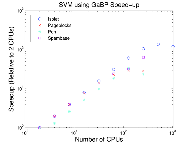
Figure 1: Speedup of the GaBP algorithm vs. 2 CPUS

Figure 1 shows the speedup results of the algorithm when running the GaBP algorithm on a Blue Gene supercomputer. The speedup with $N$ nodes is computed as the run time of the algorithm on a single node, divided by the run time using $N$ nodes. Obviously, it is desirable to obtain linear speedup, i.e., doubling computational power halves the processing time, but this is limited by the communication load and by parts of the algorithm that cannot be parallelized. Since Blue Gene is currently limited to 0.5 GB of memory at each node, most datasets could not be run on a single node. We therefore show speedup compared to two nodes. As the figure shows, in most cases we get a linear speedup up to 256 CPUs, which means that the running time is linearly proportional to one over the number of used CPUs. When using 512 - 1024 CPUs, the communication overhead reduces the efficiency of the parallel computation. We identified this problem as an area for future research into optimizing the performance for larger scale grids.

We also tested the ability to build classifiers for larger datasets. Table 3 shows the run times of the GaBP algorithm using 1024 CPUs on two larger datasets, both from the UCI repository. This demonstrates the ability of the algorithm to process very large datasets in a reasonably short amount of time. We compare our running time to state-of-the-art parallel decomposition method by Zanni et al.  [22] and Hazan et al. . Using the MNIST dataset we where considerably slower by a factor of two, but in the larger Covertype dataset we have a superior performance. Note that it is hard to compare running times since the machines used for experimentation are different. Zanni used 16 Pentium IV machines with 16Gb memory, Hazan used 10 Pentium IV machines with 4Gb memory while we used a larger number of weaker Pentium IV machines with 400Mb of memory. Furthermore, in the Covertype dataset we used only 150,000 data points while Zanni and Hazan used the full dataset which is twice larger.

Dataset	Dim	Num of examples	Run time GaBP (sec)	Run time  [22] (sec)	Run time [23]
Covertype	54	150,000/300,000	468	24365	16742
MNIST	784	60,000	756	359	18

Table 3: Running times of the GaBP solver for large data sets using 1024 CPUs on an IBM Blue Gene supercomputer. Running time results are compared to two state-of-the-art solvers:  [22] and [23].

6 Discussion

In this paper we demonstrated the application of the Gaussian Belief Propagation to the solution of SVM problems. Our experiments demonstrate the usefulness of this solver, being both accurate and scalable.

We implemented our algorithm using a synchronous communication model mainly because MPICH2 does not support asynchronous communication. While synchronous communication is the mode of choice for supercomputers such as Blue Gene, in many cases such as heterogeneous grid environments, asynchronous communication will be preferred. We believe that the next challenging goal will be to implement the proposed algorithm in asynchronous settings, where algorithm rounds will no longer be synchronized.

Our initial experiments with very large sparse kernel matrices (millions of data points) show that asynchronous settings converge faster. Recent work by Koller [3] supports this claim by showing that in many cases the BP algorithm converges faster in asynchronous settings.

Another challenging task would involve scaling to data sets of millions of data points. Currently the full kernel matrix is computed by the nodes. While this is effective for problems with many support vectors [8], it is not required in many problems which are either easily separable or else where the classification error is less important compared to the time required to learn the mode. Thus, solvers scaling to much larger datasets may have to diverge from the current strategy of computing the full kernel matrix and instead sparsify the kernel matrix as is commonly done in single node solvers.

Finally, it remains an open question whether SVMs can be solved efficiently in Peer-to-Peer environments, where each node can (efficiently) obtain data from only several close peers. Future work will be required in order to verify how the GaBP algorithm performs in such an environment, where only partial segments of the kernel matrix can be computed by each node.

References

- [1] Y. Weiss and W. T. Freeman. Correctness of belief propagation in Gaussian graphical models of arbitrary topology. In NIPS-12, 1999
- [2] J.K. Johnson. Walk-summable Gauss-Markov random fields. Technical Report, February 2002. (Corrected, November 2005).
- [3] G. Elidan and I. McGraw and D. Koller, Residual Belief Propagation: Informed Scheduling for Asynchronous Message Passing, Proceedings of the Twenty-second Conference on Uncertainty in AI (UAI), Boston, Massachussetts, 2006
- [4] J.K. Johnson, D.M. Malioutov, A.S. Willsky. Walk-sum interpretation and analysis of Gaussian belief propagation, In Advances in Neural Information Processing Systems, vol. 18, pp. 579-586, 2006.
- [5] D.M. Malioutov, J.K. Johnson, A.S. Willsky. Walk-sums and belief propagation in Gaussian graphical models, Journal of Machine Learning Research, vol. 7, pp. 2031-2064, October 2006.
- [6] Nello Cristianini and John Shawe-Taylor. An Introduction to Support Vector Machines and Other Kernel-based Learning Methods. Cambridge University Press, 2000. ISBN 0-521-78019-5.
- [7] Sethu Vijayakumar and Si Wu (1999), Sequential Support Vector Classifiers and Regression. Proc. International Conference on Soft Computing (SOCO’99), Genoa, Italy, pp.610-619.
- [8] Elad Yom-Tov (2007), A distributed sequential solver for large scale SVMs. In: O. Chapelle, D. DeCoste, J. Weston, L. Bottou: Large scale kernel machines. MIT Press, pp. 141-156.
- [9] B. Schölkopf and A. J. Smola. Learning with kernels: Support vector machines, regularization, optimization, and beyond. MIT Press, Cambridge, MA, USA, 2002.
- [10] http://www.alphaworks.ibm.com/tech/pml
- [11] Catherine L. Blake, Eamonn J. Keogh, and Christopher J. Merz. UCI repository of machine learning databases, 1998. URL http://www.ics.uci.edu/$\sim$mlearn/MLRepository.html.
- [12] R. Rifkin and A. Klautau. In defense of One-vs-All classification. Journal of Machine Learning Research, 5:101–141, 2004.
- [13] J. Dems̆ar. Statistical comparisons of classifiers over multiple data sets. Journal of Machine Learning Research, 7:1–30, 2006.
- [14] G. Zanghirati and L. Zanni. A parallel solver for large quadratic programs in training support vector machines. Parallel computing, 29:535-551, 2003.
- [15] R. Collobert, S. Bengio, and Y. Bengio. A parallel mixture of svms for very large scale problems. In Advances in Neural Information Processing Systems. MIT Press, 2002.
- [16] T. Joachims. Making large-scale svm learning practical. In ”B. Schölkopf, C. Burges, A. Smola” (Editors), Advances in Kernel Methods - Support Vector Learning,
- [17] H. P. Graf, E. Cosatto, L. Bottou, I. Durdanovic, and V. Vapnik. Parallel support vector machines: The cascade svm. In Advances in Neural Information Processing Systems, 2004.
- [18] D. Bickson, O. Shental, P. H. Siegel, J. K. Wolf, and D. Dolev. Gaussian belief propagation based multiuser detection. In IEEE Int. Symp. on Inform. Theory (ISIT), Toronto, Canada, July 2008, to appear.
- [19] O. Shental, D. Bickson, P. H. Siegel, J. K. Wolf and D. Dolev. Gaussian belief propagation solver for systems of linear equations.In IEEE Int. Symp. on Inform. Theory (ISIT), Toronto, Canada, July 2008, to appear.
- [20] D.Bickson, D. Dolev and E. Yom-Tov, Solving Large Scale Kernel Ridge Regression using A Gaussian Belief Propagation Solver in NIPS Workshop on Efficient Machine Learning, Canada, 2007.
- [21] D. Bickson, O. Shental, P. H. Siegel, J. K. Wolf, and D. Dolev. Linear detection via belief propagation, in 45th Allerton Conf. on Communications, Control and Computing, Monticello, IL, USA, Sept. 2007.
- [22] L. Zanni, T. Serafini and Gaetano Zanghirati. Parallel Software for Training Large Scale Support Vector Machines on Multiprocessor Systems. In proc of Journal of Machine Learning Research, Vol. 7 (July 2006), pp. 1467-1492.
- [23] T. Hazan, A. Man and A. Shashua. A Parallel Decomposition Solver for SVM: Distributed Dual Ascent using Fenchel Duality. In Conference on Computer Vision and Pattern Recognition (CVPR), Anchorage, June 2008, to appear.
- [24] MPI message passing interface. http://www-unix.mcs.anl.gov/mpi/mpich/