Optical pulse propagation in a switched-on photonic lattice: Rabi effect with the rôles of light and matter interchanged

Abstract

A light pulse propagating in a suddenly switched on photonic lattice, when the central frequency lies in the photonic band gap, is an analog of the Rabi model where the two-level system is the two resonant (i.e. Bragg-coupled) Fourier modes of the pulse, while the photonic lattice serves as a monochromatic external field. A simple theory of these Rabi oscillations is given and confirmed by the numerical solution of the corresponding Maxwell equations. This is a direct, i.e. temporal, analog of the Rabi effect, additionally to the spatial analog in the optical beam propagation described in Opt. Lett. 32, 1920 (2007). An additional high-frequency modulation of the Rabi oscillations reflects the lattice-induced energy transfer between the electric and magnetic fields of the pulse.

The propagation of classical waves in periodic structures has been known for a long time to exhibit intriguing analogies of the quantum phenomena, such as Bloch oscillations bloch and Zener tunneling zener . Optical demonstration of these two effects have been performed in the one-dimensional periodic structures based on waveguide arrays and superlattices falk ; morand ; italy ; india ; russia ; falk2 ; Zensplat , and recently in the two-dimensional case 2Dexp . In this letter it is shown that there is yet another type of analogy in the propagation of optical pulses in the periodic photonic lattices, where the rôles played by the light and matter are interchanged.

An optical pulse with the central frequency lying inside the photonic band gap is Bragg reflected by the lattice, which changes its spatial Fourier index by the reciprocal lattice vector. Applying the same argument to the reflected pulse, we see that there is a resonant coupling between the two optical modes with the spatial Fourier indices lying on the opposite sides of the Brillouin zone. The amplitudes of the resonant Fourier modes are subject to oscillations induced by the periodic lattice, which can be called Rabi oscillations where the optical pulse (its two resonant modes) plays the rôle of a two-level system and the photonic lattice takes the place of an external monochromatic field. Below we provide a simple theory of this effect and confirm the predictions by direct numerical simulations.

The spatial analogs of Rabi oscillations in an optical beam propagating in a photonic crystal have been previously studied RabiSch ; MCPSK (see also Ref. RabiAtom ). The temporal oscillations studied here is a direct analog of Rabi effect.

The optical pulse propagation (oblique, in general, see Fig. 1) is described by the following equations for the TE-like and TH-like pulses LL :

$$\frac{1}{\varepsilon(x)}\nabla^{2}E=\frac{1}{c^{2}}\partial^{2}_{t}E,\quad\nabla\frac{1}{\varepsilon(x)}\nabla H=\frac{1}{c^{2}}\partial^{2}_{t}H,$$ (1)

where $E=\bm{e}_{z}\bm{E}^{(TE)}$ and $H=\bm{e}_{z}\bm{H}^{(TM)}$, and $\nabla=\bm{e}_{x}\partial_{x}+\bm{e}_{y}\partial_{y}$. Below we will concentrate on the TE-like pulses, the TM-like case can be treated similarly.

The refraction index $\varepsilon(x)$ consists of the uniform component $\varepsilon_{0}$ and a periodic modulation (a weak photonic lattice), i.e.

$$\frac{1}{\varepsilon(x)}=\frac{1}{\varepsilon_{0}}\left(1+\sum_{n=-\infty}^{\infty}\hat{v}_{n}e^{2ink_{B}x}\right),$$ (2)

where $k_{B}=\pi/d$ with $d$ being the lattice period and the Fourier amplitudes of the lattice satisfy $\hat{v}_{-n}=\hat{v}_{n}^{*}$ (below, the uniform refraction index $\varepsilon_{0}$ is accounted for by introducing a modified speed of light $c_{0}=c/\sqrt{\varepsilon_{0}}$).

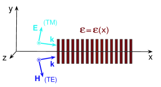
Figure 1: (Color online) Schematic setup. The electric and magnetic fields for the TE-like and TM-like pulse propagation are shown by the arrows, the photonic lattice is represented by the bars.

Equation (1) for the TE-like pulses can be considered in Fourier space by setting $E(x,y,t)=\Psi(x,t)e^{i\kappa y}$ and using the Fourier transform $\Psi=\frac{1}{2\pi}\int\mathrm{d}kC(k,t)e^{ikx}$. We get

$$-\frac{1}{c_{0}^{2}}\partial_{t}^{2}C(k,t)=\left[k^{2}+\kappa^{2}\right]C(k,t)$$

$$+\sum_{n=-\infty\atop n\neq 0}^{\infty}\hat{v}_{n}\left[(k-2nk_{B})^{2}+\kappa^{2}\right]C(k-2nk_{B},t).\qquad$$ (3)

Considering the weak lattice limit, $|\hat{v}_{1}|\ll 1$, the Bragg resonance condition for $n=1$ is satisfied for the spatial Fourier modes with peaks centered at $k_{B}$ and $-k_{B}$. Assuming the resonant initial pulse $\Psi(x,0)$ with the Fourier indices $k\in[k_{B}-\Delta k/2,k_{B}+\Delta k/2]$ we get

$$-\frac{\mathrm{d}^{2}C_{1}}{\mathrm{d}t^{2}}=\omega_{1}^{2}\left[C_{1}+\hat{v}_{1}C_{2}\right],\;-\frac{\mathrm{d}^{2}C_{2}}{\mathrm{d}t^{2}}=\omega_{2}^{2}\left[C_{2}+\hat{v}^{*}_{1}C_{1}\right],$$ (4)

where $C_{1}=C(k_{B}+\delta k,t)$ and $C_{2}=C(-k_{B}+\delta k,t)$ are the resonant Fourier modes, $\omega_{1,2}=c_{0}[(k_{B}\pm\delta k)^{2}+\kappa^{2}]^{\frac{1}{2}}$ are the corresponding frequencies, and $\delta k\in[-\Delta k/2,\Delta k/2]$, see Fig. 2. On the other hand, since Eq. (4) is the second-order system, launching a pulse with the frequencies lying in the forbidden gap is possible only by suddenly switching on the lattice. The experimental feasibility of such a setup is an open question, but possible in principle: the switch-on time is compared to the Rabi period $T_{R}\equiv 2\pi/\Omega_{0}$ with $\Omega_{0}=\omega_{0}|\hat{v}_{1}|$ (see Eq. (6) below) which is much larger than the light period.

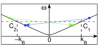
Figure 2: (Color online) Bragg resonant coupling of Fourier modes (shown by dots). The curve gives the dispersion relation $\omega(k)=c_{0}\sqrt{k^{2}+\kappa^{2}}$ (with $c_{0}=0.9$ and $\kappa=0.1$ in dimensionless units).

Consider first the simplest case with no detuning, i.e. the modes with the indices $k_{B}$ and $-k_{B}$. We have $\omega(k_{B})=\omega(-k_{B})=\omega_{0}$ and the system (4) supplemented with the initial conditions

$$C_{1}(0)=1,\;\frac{\mathrm{d}C_{1}}{\mathrm{d}t}(0)=-i\omega_{0},\;C_{2}(0)=0,\;\frac{\mathrm{d}C_{1}}{\mathrm{d}t}(0)=0,$$ (5)

corresponding to the initially propagating pulse in a homogeneous medium with $\varepsilon=\varepsilon_{0}$, can be easily solved:

$$C_{1}=\cos\left(\frac{\Omega_{0}t}{2}\right)e^{-i\omega_{0}t}+\frac{i|\hat{v}_{1}|}{4}\sin\left(\frac{\Omega_{0}t}{2}\right)e^{i\omega_{0}t},\qquad$$

$$C_{2}=e^{i\chi}\left[\sin\left(\frac{\Omega_{0}t}{2}\right)e^{-i\omega_{0}t}+\frac{i|\hat{v}_{1}|}{4}\cos\left(\frac{\Omega_{0}t}{2}\right)e^{i\omega_{0}t}\right],$$ (6)

where $\chi=\mathrm{arg}(\hat{v}_{1})-\pi/2$ and the terms of order $O(|\hat{v}_{1}|^{2})$ are omitted. The Fourier powers of the two peaks (denoted here by $|C_{1,2}|^{2}$) oscillate with the Rabi frequency $\Omega_{0}$. The oscillations are modulated with the frequency $2\omega_{0}$ and the amplitude $|\hat{v}_{1}|/4$.

The predictions have been checked by numerical simulations of Eq. (1) with the truncated expression $\varepsilon_{\mathrm{num}}(x)=\varepsilon_{0}\left[1-\hat{v}_{1}\cos\left(2\pi x/d\right)\right]$ (i.e. only the resonant terms are used). The Gaussian pulse $\Psi(x,0)=\exp\{ik_{B}x-(x-\langle x\rangle)^{2}/\sigma^{2}\}$ has been used as the initial condition. Fig. 3 shows a good comparison with the theoretical solution (6) for a pulse with the frequency interval $\Delta\omega\approx 0.07\omega_{0}=0.65\Omega_{0}$.

The sum of the Fourier powers $|C_{1}|^{2}+|C_{2}|^{2}=1-\frac{|\hat{v}_{1}|}{2}\sin(\Omega_{0}t)\sin(2\omega_{0}t)$ is not conserved since the system (4) with $\delta k=0$ has the energy

$$\mathcal{E}=\frac{1}{\omega_{0}^{2}}\left[\left|\frac{\mathrm{d}C_{1}}{\mathrm{d}t}\right|^{2}+\left|\frac{\mathrm{d}C_{2}}{\mathrm{d}t}\right|^{2}\right]+|C_{1}|^{2}+|C_{2}|^{2}+2\mathrm{Re}(\hat{v}_{1}C_{1}C^{*}_{2}).$$ (7)

For the solution (6) one can neglect the term Re$\left(\hat{v}_{1}C_{1}C^{*}_{2}\right)=O(|\hat{v}_{1}|^{2})$. Hence, there are oscillations between the sum $|C_{1}|^{2}+|C_{2}|^{2}$ and the analogous sum of the time derivatives of $C_{1,2}$, with the two frequencies $\omega_{0}\pm\Omega_{0}/2$, corresponding to the lower and upper band-gap ends, and with the amplitude $|\hat{v}_{1}|/4$. The oscillations reflect the transfer of the electromagnetic energy between the electric and magnetic fields. The Rabi oscillations can be traced also in the real space, where they appear in the form of pulse average position oscillations, see Fig 4(a). The pulse is also spreading (Fig. 4(b)) and propagating with a small group velocity.

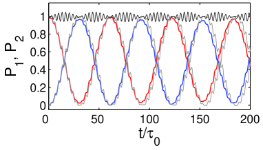
Figure 3: (Color online) The average Fourier powers $P_{1,2}$ (see Eq. (10) below) of the numerical solution of Eq. (1), the thick lines, vs the theoretical solution (6) with no detuning, the thin line. The upper line gives the sum of powers $P_{1}+P_{2}$. Here $\tau_{0}=(c_{0}k_{B})^{-1}$, $\varepsilon_{0}=1.3$, $\hat{v}_{1}=0.12$, and $\kappa=0.05k_{B}$. The Gaussian initial pulse is used with the width $\sigma=34d$, hence $\Delta k=0.04k_{B}$, i.e. $\Delta\omega=0.65\Omega_{0}$.

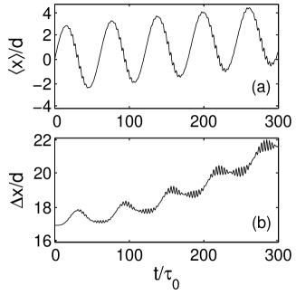
Figure 4: The pulse average position, defined as $\langle x\rangle=\int\mathrm{d}x\,x|E|^{2}/\int\mathrm{d}x\,|E|^{2}$ panel (a), and its half-width, $(\Delta x)^{2}=\int\mathrm{d}x\,(x-\langle x\rangle)^{2}|E|^{2}/\int\mathrm{d}x\,|E|^{2}$, panel (b), corresponding to Fig. 3.

As one would expect, for shorter pulses than that of Fig. 3 the oscillations show such features as the dephasing and the amplitude damping, since there is a frequency detuning between the resonant Fourier modes $k$ and $k-2k_{B}$ ($k\neq k_{B}$), see Fig. 2. In the general case, the two resonant modes in Eq. (4), i.e. $C_{1}(t)=C(k_{B}+\delta k,t)$ and $C_{2}(t)=C(-k_{B}+\delta k,t)$, have the following form (up to the $O(|\hat{v}_{1}|)$-terms)

$$C_{1} = e^{-i\overline{\omega}t}\left[\cos\left(\frac{\Omega t}{2}\right)-i\frac{\gamma}{\sqrt{1+\gamma^{2}}}\sin\left(\frac{\Omega t}{2}\right)\right],$$

$$C_{2} = e^{i\chi-i\overline{\omega}t}\frac{1}{\sqrt{1+\gamma^{2}}}\sin\left(\frac{\Omega t}{2}\right),$$ (8)

where

$$\overline{\omega}=\sqrt{\frac{\omega_{1}^{2}+\omega_{2}^{2}}{2}},\;\Omega=\overline{\omega}|\hat{v}_{1}|\sqrt{1+\gamma^{2}},\;\gamma=\frac{\omega_{1}^{2}-\omega_{2}^{2}}{\omega_{1}^{2}+\omega_{2}^{2}}\frac{1}{|\hat{v}_{1}|}.$$ (9)

Since the small $O(|\hat{v}_{1}|)$-terms are neglected, the total power is conserved in Eq. (8) $|C_{1}|^{2}+|C_{2}|^{2}=1$. Both the amplitude of oscillations and the frequency are defined by the ratio $\gamma\approx\frac{\delta\omega}{\overline{\omega}|\hat{v}_{1}|}\approx\frac{\delta\omega}{\Omega_{0}}$ of the frequency detuning to the band-gap width. Averaging over an interval of the size $\Delta k$ and evaluating the integral by the stationary phase method, one obtains for $t\gg 1$:

$$P_{1,2} \equiv \frac{1}{\Delta k}\int\limits_{\pm k_{B}-\Delta k/2}^{\pm k_{B}+\Delta k/2}\mathrm{d}\lambda|C(\lambda,t)|^{2}$$ (10)

$$= \frac{1}{2}\left\{1\pm\frac{\Omega_{0}}{\Delta\omega}\sqrt{\frac{\pi}{\Omega_{0}t}}\cos(\Omega_{0}t+\pi/4)\right\},\quad$$

where $\Delta\omega=\omega(k_{B}+\Delta k/2)-\omega(-k_{B}+\Delta k/2)$.  An example of the Rabi oscillations with a large detuning (i.e. for a short pulse) is given in Fig. 5. In this case, the average position of the pulse and the pulse width show nearly linear dependence on time, the pulse spreads and propagates in the lattice significantly.

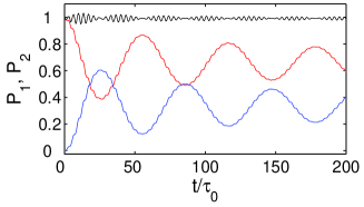
Figure 5: (Color online) The average Fourier powers $P_{1,2}$ of the numerical solution of Eq. (1) and their sum (the upper line). The difference from Fig. 3 is in the pulse width $\sigma=6d$ which gives $\Delta k=0.11k_{B}$, i.e. $\Delta\omega=0.22\omega_{0}=1.9\Omega_{0}$.

In conclusion, an electromagnetic pulse propagation in a switched-on photonic lattice with the central frequency lying in the forbidden gap is an analog of the Rabi model, where the two-level media is the pulse, i.e. its two resonant Fourier modes, while the photonic lattice serves as a classical monochromatic field. The Rabi frequency is given by the band-gap width and the oscillations have all the characteristic features as in the original Rabi case, such as the amplitude damping due to the dephasing. An additional feature is the high-frequency modulation of the oscillations due to the energy transfer between the electric and magnetic fields of the pulse. The effect may have applications, for instance, as a base for an all-optical trap for light pulses.

This work has been supported by the CAPES and FAPESP of Brasil. The author acknowledges the hospitality of Gleb Wataghin Institute of Physics at UNICAMP in Brazil, where he has benefited from illuminating discussions with L. E. Oliveira and S. B. Cavalcanti.

References

(1) F. Bloch, Z. Phys. A: Hadrons
Nucl. 52, 555 (1928) (in German).
(2) C. Zener, Proc. R. Soc. A 145, 523 (1934).
(3) T. Pertsch, P. Dannberg, W. Elflein, and A. Bräuer, and F. Lederer, Phys. Rev. Lett. 83, 4752 (1999).
(4) R. Morandotti, U. Peschel, J. S. Aitchison, H. S. Eisenberg and
Y. Silberberg, Phys. Rev. Lett. 83, 4756 (1999).
(5) R. Sapienza, P. Costantino, D. Wiersma, M. Ghulinyan, C. J. Oton, and L. Pavesi, Phys. Rev. Lett. 91, 263902 (2003).
(6) V. Agarwal, J. A. del Río, G. Malpuech,
M. Zamfirescu, A. Kavokin, D. Coquillat, D. Scalbert, M. Vladimirova, and B. Gil,
Phys. Rev. Lett. 92, 097401 (2004).
(7) B. A. Usievich, V. A. Sychugov, J. Kh. Nirligareev, and K. M. Golant, Opt. Spectrosc. 97, 790 (2004).
(8) H. Trompeter, Th. Pertsch, F. Lederer, D. Michaelis, U. Streppel, A. Bräuer, and U. Peschel, Phys. Rev. Lett. 96, 023901 (2006).
(9) M. Ghulinyan, C. J. Oton, Z. Gaburro, L. Pavesi, C. Toninelli, and D. S. Wiersma,
Phys. Rev. Lett. 94, 127401 (2005).
(10) H. Trompeter, W. Krolikowski, D. N. Neshev, A. S. Desyatnikov, A. A. Sukhorukov, Yu. S. Kivshar, Th. Pertsch, U. Peschel,
and F. Lederer, Phys. Rev. Lett. 96, 053903 (2006).
(11) V. S. Shchesnovich and S. Chàvez-Cerda, Opt. Lett. 32, 1920
(2007).
(12) K. G. Makris, D. N. Christodoulides, O. Peleg, M. Segev and D. Kip,
Opt. Express 16, 10309 (2008).
(13) A. S. Mellish, G. Duffy, C. McKenzie, R. Geursen, and A. C.
Wilson, Phys. Rev. A 68, 051601(R) (2003)
(14) L. D. Landau and E. M. Lifshitz, Electrodynamics of Continuous
Media, (Pergamon Press, 1960).