Fluctuation-Dissipation relation in sub-diffusive systems: the case of granular single-file

Abstract

We study a gas of hard rods on a ring, driven by an external thermostat, with either elastic or inelastic collisions, which exhibits sub-diffusive behavior $\langle x^{2}\rangle\sim t^{1/2}$. We show the validity of the usual Fluctuation-Dissipation (FD) relation, i.e. the proportionality between the response function and the correlation function, when the gas is elastic or diluted. On the contrary, in strongly inelastic or dense cases, when the tracer velocity is no more independent of the other degrees of freedom, the Einstein formula fails and must be replaced by a more general FD relation.

Introduction

The typical scenario in diffusive problem is the so called standard diffusion, which is qualitatively similar to the usual behaviour in the Brownian motion, i.e. at large time one has

$$\langle x(t)^{2}\rangle\simeq 2Dt\,\,,$$ (1)

where $D$ is the diffusion coefficient which is linked to the velocity correlation function via the Kubo formula

$$D=\int_{0}^{\infty}\langle v(t)v(0)\rangle dt\,.$$

Of course the above scenario holds if $\int_{0}^{\infty}\langle v(t)v(0)\rangle dt$ is finite and non-zero.

On the other hand, it is well known that, beyond the standard diffusion, one can have anomalous diffusion [1, 2], i.e.

$$\langle x^{2}(t)\rangle\sim t^{2\nu}\,\,\,\mbox{with}\,\,\,\nu\neq 1/2,$$ (2)

formally this corresponds to have $D=\infty$ if $\nu>1/2$ (superdiffusion) and $D=0$ if $\nu<1/2$ (subdiffusion).

From the well estabished linear response theory, it is known that, when $\langle x(t)\rangle=0$ in the unperturbed system, (1) implies a linear drift

$$\overline{x(t)}\sim t\,\,,$$ (3)

if a small external force is applied [3, 4]. In the following we will indicate with $\langle\cdot\rangle$ the average in the unperturbed system, i.e. weighting states according to the stationary phase-space distribution and with $\overline{(\cdot)}$ the time dependent average in the dynamical ensemble generated by the external perturbation. One can wonder how Eq. (3) changes in presence of anomalous diffusion, i.e. if, instead of (1), eq. (2) holds.

The “usual” fluctuation-dissipation relation relates the mean response $R(t)=\frac{\overline{\delta v(t)}}{\delta v(0)}$ at time $t$ of the velocity after an impulsive infinitesimal perturbation $\delta v(0)$, applied at time $t=0$, to the velocity autocorrelation $C_{v}(t_{1}-t_{2})=\langle v(t_{1})v(t_{2})\rangle$:

$$R(t)=C_{v}(t)/C_{v}(0).$$

When an infinitesimal force is applied for positive times, one has

$$\overline{v(t)}={d\over dt}\overline{x(t)}\propto\int_{0}^{t}C_{v}(t^{\prime})dt^{\prime}\,\,.$$ (4)

A straigthforward consequence of the above relations and of the simple identity

$$\langle x^{2}(t)\rangle=\int_{0}^{t}\int_{0}^{t}C_{v}(t_{1}-t_{2})dt_{1}dt_{2}\,\,\,\,,\,\,\,\,$$ (5)

which suggests

$$\overline{x(t)}=\int_{0}^{t}\overline{v(t)}dt\propto\langle x^{2}(t)\rangle\sim t^{2\nu}\,\,,$$ (6)

in analogy with (3). On the other hand, it can be seen that such a formal argument is not rigorous and the actual scenario may become rather subtle, see e.g. [5]. For a detailed discussion the reader can see [4].

In this paper we discuss the subdiffusive situation. Some works show that in such a case the expected result (6) seems to hold [6, 7]. This has been explicitely proved in systems described by a fractional-Fokker-Planck [7] equation, where a generalized Einstein relation has been shown ($F$ is the perturbing force).

$$\overline{x(t)}={1\over 2}{F\langle x^{2}(t)\rangle\over k_{B}T}\,\,.$$ (7)

Models based on fractional Fokker-Planck equations, although interesting, usually are not directly derived from specific real systems; we therefore wondered whether a relation similar to (7) holds in more realistic models, such as in single file diffusion [8], which is a sub-diffusive system having many realizations in nature (e.g. transport in nanopores or narrow channels and zeolites, as well as car traffic on single lanes, pedestrian dynamics, etc.). The model used here consists of a one-dimensional gas of inelastic hard particles, moving on a large ring. To ensure a stationary state, particles exchange energy with an external thermostat. Tuning the characteristic time of the thermostat, the average volume fraction occupied by the gas and the restitution coefficient (from elastic to completely anelastic), one may observe a wide range of different stationary states, from a homogeneous density with Gaussian velocity distribution to strongly inhomogeneous spatial arrangement (clustering) with non-Gaussian statistics of velocities [9, 10, 11, 12, 13]. Other authors have studied diffusion in granular gases without any external driving: in this case the gas is non-stationary (cooling regime) and one finds non-trivial exponents for diffusion [14, 15].

The aim of this paper is to discuss the consequences of both subdiffusion and inelasticity in the more general context of linear response theory for statistically stationary states [16, 17]. Let us briefly remind some general results [4]. Consider a dynamical system ${\bf X}(0)\to{\bf X}(t)=U^{t}{\bf X}(0)$ whose time evolution can also be not completely deterministic (e.g. stochastic differential equations), with states ${\bf X}$ belonging to a $N$-dimensional vector space. We assume a) the existence of an invariant probability distribution $\rho({\bf X})$, for which an “absolute continuity” condition is required (see [4] for details), and b) the mixing character of the system (from which its ergodicity follows). In our stochastic model the two above requests hold. Under these hypotheses, it is possible to derive (for details see [16, 17, 4]) the following generalized FD relation, valid when considering the perturbation at time $0$ of a coordinate $X_{j}$:

$$R_{i,j}(t)=\frac{\overline{\delta X_{i}(t)}}{\delta X_{j}(0)}=-\Biggl{\langle}X_{i}(t)\left.\frac{\partial\ln\rho({\bf X})}{\partial X_{j}}\right|_{t=0}\Biggr{\rangle}\,.$$ (8)

In the case of thermostatted Hamiltonian systems, on the other side, one has that $\rho({\bf q},{\bf p})\propto\exp(-\beta\mathcal{H}({\bf q},{\bf p}))$. From formula (8),therefore, one has that

$$R_{V,V}=\frac{\langle V(t)V(0)\rangle}{\langle V(0)^{2}\rangle}.$$ (9)

With a slight abuse of terminology, we will use the form “Einstein relation” to denote the time dependent Eq. (9). Let us note that its validity is a consequence of the Gaussian statistics of the velocity and the factorization of the stationary probability distribution, i.e. positions and velocities are independent. In non-Hamiltonian systems, the shape of $\rho({\bf x})$ is not known in general, therefore (8) does not give a straightforward information. Nevertheless it can be exploited to get an interpretation of the results of a linear response experiment. We will analyze the response to small perturbations in the stationary state of a one-dimensional granular gas, discussing the response properties of the stationary state with its many “anomalies” with respect to an equilibrium state.

We stress that the regimes considered here are always ergodic: this is a relevant difference with respect to the studies on the violations of the Fluctuation-Response relation, which considered glassy systems in the non-ergodic (aging) phase [18].

The model

The model considered here consists of a gas of $N$ inelastic hard rods of mass $1$, of linear size $d$, moving on a ring of length $L$. The rods interact also with a heating bath which mimics the effect of an irregular vibration injecting energy in the system. Until a collision occurs, the position $x_{i}$ and the velocity $v_{i}$ of $i$-th rod obeys the following equations:

$$\frac{dx_{i}(t)}{dt}=v_{i}(t),\;\;\;\;\;\;\frac{dv_{i}(t)}{dt}=-\frac{v_{i}}{\tau_{b}}+\sqrt{\frac{2T_{b}}{\tau_{b}}}\eta_{i}(t),$$ (10)

where $\eta_{i}(t)$ is a Gaussian white noise with $\langle\eta_{i}(t)\rangle=0$ and $\langle\eta_{i}(t)\eta_{j}(t^{\prime})\rangle=\delta_{ij}\delta(t-t^{\prime})$. When two rods $i$ and $j$ come into contact, their velocities $v_{i}$ and $v_{j}$ are instantaneously changed into $v_{i}^{\prime}$ and $v_{j}^{\prime}$ with the following rule:

$$v_{i}^{\prime}=v_{i}-\frac{1+r}{2}(v_{i}-v_{j}),\;\;\;\;\;\;\;v_{j}^{\prime}=v_{j}+\frac{1+r}{2}(v_{i}-v_{j}).$$ (11)

The meanings of $\tau_{b}$ and $T_{b}$ are those of a typical thermalization time and a temperature, respectively, obtained if the system is elastic ($r=1$). The coefficient of restitution $r\in[0,1]$ determines the degree of inelasticity: after a collision, a fraction proportional to $1-r^{2}$ of the relative kinetic energy (i.e. kinetic energy in the center of mass frame) of the two particles is lost. When the particles are homogeneously distributed along the ring, the mean free path is given by $\lambda=1/n-d=(1-\phi)/n$ where $n=N/L$ is the number density and $\phi=nd$ is the occupied volume fraction. The mean free time $\tau_{c}$ is roughly estimated as $\lambda/\sqrt{T_{g}}$. In the rest of the paper we will tune $n$ or $\tau_{b}$, keeping fixed $T_{b}=1$, in order to change the ratio between characteristic times $\alpha=\tau_{c}/\tau_{b}$. For any value of $r$ or $\alpha$, the system reaches a statistically stationary regime where a kinetic temperature, denoted as “granular temperature”, $T_{g}=\langle v^{2}\rangle$ can be measured. When $\alpha\gg 1$, the coupling with the thermostat dominates the dynamics of the rods: they therefore remain thermalized and the system results at equilibrium at temperature $T_{b}$: only spatial (rod-rod) correlations are expected at equilibrium, while velocities are not correlated, i.e. the global phase space probability distribution function (pdf) factorizes as:

$$\rho(\{x_{i}\},\{v_{i}\})=\rho_{x}(\{x_{i}\})\prod_{i=1}^{N}p_{v}(v_{i}),$$ (12)

with $p_{v}(v)$ a Gaussian distribution with variance $T_{b}$. On the contrary, when $\alpha\ll 1$, the effect of inelastic collision is strong enough to draw the system in a non-equilibrium stationary state whose properties are known from previous studies [9, 10, 11, 12, 13]. Non-Gaussian single particle velocity distributions and correlations among velocities and positions are the most relevant; these anomalies with respect to equilibrium become more and more pronounced as $\alpha$ or $r$ are reduced. As a matter of fact, in this regime it is not correct to assume a factorization of the kind of Eq. (12), and the single particle velocity distribution, which is non-Gaussian, represents only a projection on a single degree of freedom of the full phase-space measure. We will see that the non-gaussianity of velocities is by far less important that the lack of factorization, which becomes relevant when the system is not dilute enough and which makes the Einstein relation (9) fail.

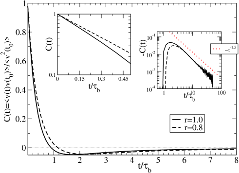
Figure 1: Plot of the normalized autocorrelation $C(t)$ versus time, for two cases, one elastic (full line) and the other inelastic (dashed line). In the left inset we show a blow-up of the exponential decay at early times. In the right inset you can find a blow up in log-log scale of the negative tail, together with a power law decay $t^{-3/2}$. Here $\phi=0.1$, and $\alpha\approx 0.9$.

The velocity autocorrelation function

In Figure 1 we show the normalized autocorrelation function: $C(t)=C_{v}(t)/C_{v}(0)=\langle v(t)v(0)\rangle/T_{g}$ for the velocity of a tagged particle (a tracer with the same properties of other particles). In both elastic and inelastic experiments, $C(t)$ presents three main features: a) an exponential decay at early times, b) a negative minimum and c) asymptotically a power-law decay $C(t)\sim-t^{-3/2}$. The negative minimum is necessary to have subdiffusion, i.e. $D=\int_{0}^{\infty}C(t)=0$, while the final power-law decay with $3/2$ exponent is necessary to have $\langle x^{2}(t)\rangle\sim t^{1/2}$. The initial exponential decay $C(t)\sim\exp(-t/t_{corr})$ has a more subtle nature. In $1D$ one can argue that the tracer “discovers” the geometrical contraint after a long time. However, calculations based on collisions between non-correlated particles lead to wrong predictions for $t_{corr}$. Since this point is not closely related to the FD relation, we do not discuss it in detail. Here we do not show the mean squared displacement as a function of time, already detailed in [19]: however the single-file diffusion scenario $\langle x^{2}(t)\rangle\sim t^{1/2}$ holds for any value of $r$, $\alpha$ and $\phi$.

The response to an impulsive perturbation

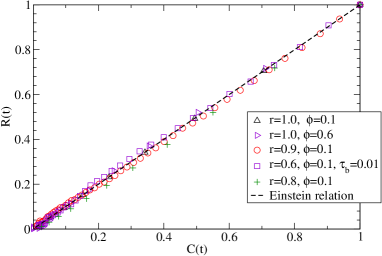
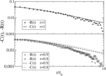
Figure 2: Left: parametric plot of response $R(t)$ versus normalized autocorrelation $C(t)$. The dashed line marks the Einstein relation $R\equiv C$. Where not specified, $\tau_{b}=1$. Right: $-C(t)$ and $-R(t)$ versus $t$ for elastic and inelastic cases at late times, with $\phi=0.1$ and $\tau_{b}=1$.

The response to an impulsive perturbation is shown in Figure 2 for some choices of parameters. We have used a standard recipe to have a clean measure of response [20]: the system is let thermalize, then at time $t_{0}$ is cloned. The original system evolves without perturbation, the copy is perturbed, i.e. the tagged tracer receives a small kick $v(t_{0})\to v^{\prime}(t_{0})=v(t_{0})+\delta v$ with $\delta v\ll\sqrt{T_{g}}$ to ensure linearity of the response. Then the copy is evolved using the same noise realization as for the original system and the response is given by the dynamical average $R(t)=\overline{(v^{\prime}(t_{0}+t)-v(t_{0}+t))}/\delta v$ over many realizations of the experiment. In Figure 2 we show representative cases where the Einstein relation $R(t)=C(t)$ is verified within numerical precision. This happens for elastic cases, or cases at low inelasticity $1-r\ll 1$ and low packing fraction, and also for cases at high inelasticity, provided that $\tau_{b}\ll\tau_{c}$. This last setup corresponds to a very fast action of the thermal bath which practically removes the effects of inelastic collisions. Similar results have been obtained, previously, for $2d$ driven granular gases [21, 22, 23, 24, 25]. As shown in the top-right frame, for the elastic case, the relation $R(t)=C(t)$ is fairly verified also at late times in the power-law tail. The inelastic case (see bottom-right frame) displays a small violation at such large times: note that this small violation corresponds to both $R(t)$ and $C(t)$ very close to zero.

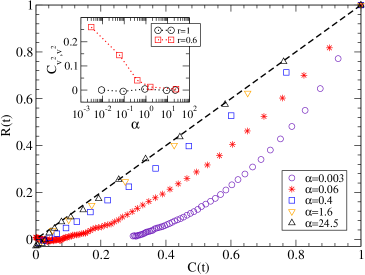
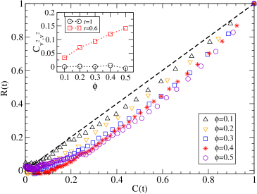
Figure 3: Parametric plot of response $R(t)$ versus normalized autocorrelation $C(t)$. The dashed line is the Einstein relation $R\equiv C$. All data are obtained with restitution coefficient $r=0.6$. On the left: the packing fraction is constant $\phi=0.1$ and $\tau_{b}$ is changed, resulting in different values of $\tau_{c}$. The ratio $\alpha=\tau_{c}/\tau_{b}$ is given for simplicity. On the right: $\tau_{b}=1$ is kept constant, while $\phi$ is changed. In the insets the correlator $C_{v^{2},v^{2}}$, discussed in the text, is displayed as a function of the varying parameter, for elastic and inelastic systems.

In Figure 3 the parametric plot of response versus correlation is displayed for cases where the Einstein relation is no more verified. The departure from the equality $R(t)=C(t)$ can be quite strong: it increases with the packing fraction $\phi$, the inelasticity $1-r$ and the rescaled bath time $\tau_{b}/\tau_{c}=1/\alpha$. In all cases we observe $R(t)<C(t)$. In Fig. 3 we have stressed the dependence on $\alpha$, which can be tuned changing $\tau_{b}$ at fixed $r$ and $\phi$. In all experiments we have verified to be in the linear response regime.

Origin of the violation of the Einstein relation

As anticipated in the description of the model, and in agreement with the observation done in [25], the Einstein relation no more holds when the factorization of the phase-space pdf expressed by Eq. (12) is violated. For reasons of space we do not show the probability density function of one-particle velocities, which are not far from the Maxwell-Boltzmann distribution. Violations of Gaussianity have been shown in [25] to be not relevant for the FD relation, because autocorrelations at different orders are almost proportional, i.e. $\langle v(0)v(t)\rangle/\langle v^{2}\rangle\approx\langle v(0)^{2}v(t)\rangle/\langle|v|^{3}\rangle\approx\langle v(0)^{3}v(t)\rangle/\langle v^{4}\rangle$ etc. This is confirmed by Direct Monte Carlo simulations, where an almost perfect factorization of the degrees of freedom in the phase-space pdf is satisfied: in such simulations, even with a stronger departure from Gaussianity, the Einstein relation always holds.

Many ways of characterizing the breakdown of phase-space factorization can be employed. A simple one is displayed in the inset of Fig. 3:

$$C_{v^{2},v^{2}}=\frac{\langle\delta v_{i}^{2}\delta v^{2}_{i+1}\rangle}{\langle\delta v_{i}^{4}\rangle},$$ (13)

where $\delta v_{i}^{2}=v_{i}^{2}-T_{g}$. When $C_{v^{2},v^{2}}>0$, the squared velocities of two adjacent particles are correlated. It is evident that this correlation increases when $\alpha$ is decreased. The same is observed tuning the other parameters, such as decreasing $r$ or increasing $\phi$.

Conclusions

Drawing the conclusions, we stress the twofold nature of this study. On one side, for the elastic single-file diffusion, which is a less abstract model than fractional Fokker-Planck, we have obtained a good agreement between $R(t)$ and $C(t)$, in all time ranges, confirming the validity of the FD (“Einstein”) relation. On the other side we have explored the effects of inelasticity: in this case one has a non-equilibrium stationary state where strong correlations among different particles are present, therefore the factorization (12) fails and only a more general FD relation (8) holds. At small inelasticity, small packing fraction and/or for fast thermostats, the Einstein relation is recovered, because the lack of factorization is weak, as previously observed in $2d$ granular gases [21, 22, 26, 23, 24, 25]. A quantitative characterization of the departure from factorization is under investigation, with the aim of proposing, as a first step, a joint two-particles (first neighbours) velocity distribution: we expect to obtain, from this study, a first explicit correction formula to the Einstein relation.

References

- [1] G M Zaslavsky, D Stevens, and H Weitzner. Self-similar transport in incomplete chaos. Phys. Rev. E, 48:1683, 1993.
- [2] P Castiglione, A Mazzino, P Muratore-Ginanneschi, and A Vulpiani. On strong anomalous diffusion. Physica D, 134:75, 1999.
- [3] R Kubo. The fluctuation-dissipation theorem. Rep. Prog. Phys., 29:255, 1966.
- [4] U Marini Bettolo Marconi, A Puglisi, L Rondoni, and A Vulpiani. Fluctuation-dissipation: Response theory in statistical physics. Phys. Rep., 461:111, 2008.
- [5] G Trefan, E Floriani, B J West, and P Grigolini. Dynamical approach to anomalous diffusion: Response of Levy processes to a perturbation. Phys. Rev. E, 50:2564, 1994.
- [6] E. Barkai and J. Klafter. Comment on subdiffusion and anomalous local viscoelasticity in actin networks”. Phys. Rev. Lett., 81:1134, 1998.
- [7] R Metzler, E Barkai, and J Klafter. Anomalous diffusion and relaxation close to thermal equilibrium: A fractional Fokker-Planck equation approach. Phys. Rev. Lett, 82:3563, 1999.
- [8] D. G. Levitt. Dynamics of a single-file pore: Non-fickian behavior. Phys. Rev. A, 8:3050, 1973.
- [9] D R M Williams and F C MacKintosh. Driven granular media in one dimension: Correlations and equation of state. Phys. Rev. E, 54:R9, 1996.
- [10] A Puglisi, V Loreto, U M B Marconi, A Petri, and A Vulpiani. Clustering and non-gaussian behavior in granular matter. Phys. Rev. Lett., 81:3848, 1998.
- [11] A Puglisi, V Loreto, U M B Marconi, and A Vulpiani. A kinetic approach to granular gases. Phys. Rev. E, 59:5582, 1999.
- [12] T P C van Noije and M H Ernst. Velocity distributions in homogeneous granular fluids: the free and the heated case. Granular Matter, 1:57–64, 1998.
- [13] T P C van Noije, M H Ernst, E Trizac, and I Pagonabarraga. Randomly driven granular fluids: Large-scale structure. Phys. Rev. E, 59:4326, 1999.
- [14] N V Brilliantov and T Poschel. Self-diffusion in granular gases. Phys. Rev. E, 61:1716, 2000.
- [15] J J Brey, M J Ruiz-Montero, D Cubero, and R Garc a-Rojo. Self-diffusion in freely evolving granular gases. Phys. Fluids, 12:876, 2000.
- [16] U Deker and F Haake. Fluctuation-dissipation theorems for classical processes. Phys. Rev. A, 11:2043, 1975.
- [17] M Falcioni, S Isola, and A Vulpiani. Correlation functions and relaxation properties in chaotic dynamics and statistical mechanics. Physics Letters A, 144:341, 1990.
- [18] J P Bouchaud, L F Cugliandolo, J Kurchan, and M Mezard. Spin Glasses and Random Fields. World Scientific, 1998.
- [19] F Cecconi, F Diotallevi, U Marini Bettolo Marconi, and A Puglisi. Fluid-like behavior of a one-dimensional granular gas. J. Chem. Phys., 120:35, 2004.
- [20] G. Ciccotti, G. Jacucci, and I.R. McDonald. ”Though- Experiments” by molecular dynamics. J. Stat. Phys., 21:1, 1979.
- [21] A Puglisi, A Baldassarri, and V Loreto. Fluctuation-dissipation relations in driven granular gases. Physical Review E, 66:061305, 2002.
- [22] A Barrat, V Loreto, and A Puglisi. Temperature probes in binary granular gases. Physica A, 334:513, 2004.
- [23] V Garzó. On the Einstein relation in a heated granular gas. Physica A, 343:105, 2004.
- [24] A Baldassarri, A Barrat, G D’Anna, V Loreto, P Mayor, and A Puglisi. What is the temperature of a granular medium? Journal of Physics: Condensed Matter, 17:S2405, 2005.
- [25] A Puglisi, A Baldassarri, and A Vulpiani. Violations of the Einstein relation in granular fluids: the role of correlations. J. Stat. Mech., page P08016, 2007.
- [26] Y Srebro and D Levine. Exactly solvable model for driven dissipative systems. Phys. Rev. Lett., 93:240601, 2004.