SFB/CPP-08-74 TTP08-43
${\cal O}(\alpha\alpha_{s})$ corrections to the $\gamma t\bar{t}$ vertex at the top quark threshold

Abstract

We compute the last missing piece of the two-loop ${\cal O}(\alpha\alpha_{s})$ corrections to $\gamma t\bar{t}$ vertex at the $t\bar{t}$ threshold due to the exchange of a $W$ boson and a gluon. This contribution constitutes a building block of the top quark threshold production cross section at electron positron colliders.

PACS numbers:12.38.Bx,12.15.-y,12.38.-t,14.65.Ha

1 Introduction

The top quark pair production close to the threshold is an important process at a future International Linear Collider (ILC). It can be used to determine top quark properties, like the mass $m_{t}$ and the width $\Gamma_{t}$, but also the strong coupling $\alpha_{s}$ with high precision. This is in particular true for $m_{t}$ where an uncertainty below 100 MeV can be obtained from a threshold scan of the cross section [1].

The feasibility of such high-precision measurements requires a theory prediction of the total cross section $\sigma(e^{+}e^{-}\rightarrow t\bar{t})$ with high accuracy (preferably $\delta\sigma/\sigma\leq 3\%$). Current estimates based on (partial) next-to-next-to-leading logarithmic (NNLL) order [2, 3] and (partial) next-to-next-to-next-to-leading order (NNNLO) [4, 5] QCD corrections lead to an uncertainty of the order of 10%.

In order to reach a theory goal of $\delta\sigma/\sigma\leq 3\%$ it is necessary to include in the prediction next to the one-loop electroweak corrections, which are known since quite some time [6] (see also [7]), also higher order effects. The evaluation of ${\cal O}(\alpha\alpha_{s})$ corrections has been started in Ref. [8], where the two-loop mixed electroweak and QCD corrections to the matching coefficient of the vector current has been computed due to a Higgs or $Z$ boson exchange in addition to a gluon. The current paper continues this enterprise and provides a result of ${\cal O}(\alpha\alpha_{s})$ for the two-loop vertex diagrams mediated by a $W$ boson and gluon exchange. This completes the vertex corrections of order $\alpha\alpha_{s}$ — a building block for the top quark production cross section. Assuming the (numerically well justified) power counting $\alpha\sim\alpha_{s}^{2}$ one can see that these corrections are formally of NNNLO.

In order to complete the matching corrections of order $\alpha\alpha_{s}$ also the two-loop box diagrams contributing to $e^{+}e^{-}\to t\bar{t}$ have to be considered. Actually, only the proper combination of the box, vertex and self-energy contributions (the latter can, e.g., be found in Refs. [9, 10]) forms a gauge independent set.

The remainder of the paper is organized as follows: In the next Section we introduce our notation and derive the cross section formula for $e^{+}e^{-}\rightarrow t\bar{t}X$ near the $t\bar{t}$ threshold. We present a general formula which includes all radiative corrections of the Standard Model (SM). In Section 3 we discuss some technical details of the two-loop computation and in Section 4 we concentrate on the ${\cal O}(\alpha\alpha_{s})$ corrections to the $\gamma t\bar{t}$ vertex and present our results. Section 5 contains our conclusions. Additional useful material concerning the one-loop expressions can be found in the Appendix.

2 Threshold cross section

The production cross section for the process $e^{+}e^{-}\to t\bar{t}X$ near threshold consists of helicity amplitudes and the hadronic part. The former correspond to the high-energy production amplitude of a top quark pair, the latter to the QCD bound-state dynamics of the produced $t\bar{t}$ pairs exchanging gluons to form a resonance. The cross section can be cast in the form (for left-landed positrons and right-handed electrons),

$$R\left(e_{L}^{+}e_{R}^{-}\rightarrow t\bar{t}X\right) = \frac{8\pi}{s}\,{\rm Im}\big{[}\,\left(h_{R,\,V}\right)^{\,2}H_{V}+\left(h_{R,\,A}\right)^{\,2}H_{A}\big{]}\,,$$ (1)

where $s$ is the square of the center-of-mass energy and $R(e_{L}^{+}e_{R}^{-}\rightarrow t\bar{t}X)$ is the cross section normalized to $\sigma(e^{+}e^{-}\rightarrow\mu^{+}\mu^{-})=(4\pi\alpha^{2})/(3s)$. The first subscript of $h$ refers to helicity of the electron, and the second one to the vector ($J_{V}^{\mu}=\bar{\psi}\gamma^{\mu}\psi$) or axial-vector coupling ($J_{A}^{\mu}=\bar{\psi}\gamma^{\mu}\gamma_{5}\psi$) of the gauge bosons to the top quark current. For $e^{+}_{R}e^{-}_{L}$ in the initial state a similar expression is obtained by replacing R by L in Eq. (1). In the SM the helicity amplitudes for $e^{+}_{R}e^{-}_{R}$ and $e^{+}_{L}e^{-}_{L}$ are proportional to $m_{e}/M_{W}\sim 10^{-5}$ and are thus negligible.

In the cross section formula (1) “${\rm Im}$” refers to those cuts which correspond to the $t\bar{t}X$ final state. This means that we have to select special cuts which correspond to the final state we are interested in. This requires a dedicated study incorporating the experimental setup. For the one-loop electroweak correction this treatment was performed in [11]. In this paper we will not pursue this problem further (see also the discussion in the Conclusions).

The hadronic part is described by non-relativistic QCD (NRQCD) [12]. For our purpose it is sufficient to re-write the vector current $J_{V}^{\mu}$ and the axial-vector current $J_{A}^{\mu}$ in terms of two-component NRQCD spinor fields $\psi$, $\chi$, which correspond to non-relativistic top and anti-top quarks, respectively. This yields the following NRQCD currents

$$j_{V}^{\,i}=\psi^{\dagger}\,\sigma^{i}\chi,~{}~{}~{}j_{V}^{(1/m^{2}),\,i}=-\frac{1}{6m_{t}^{2}}\psi^{\dagger}\,\sigma^{i}(i{\vec{D}}\,)^{2}\,\chi,~{}~{}~{}j_{A}^{\,i}=\frac{1}{2m_{t}}\,\psi^{\dagger}\,[\sigma^{i},\left({\vec{\sigma}}\,i{\vec{D}}\,\right)]\,\chi\,.$$ (2)

With the help of the NRQCD equation of motion for top and anti-top quarks ($\psi^{\dagger}\sigma^{i}\,{\vec{D}\,}^{2}\chi=m_{t}\,i\partial_{0}(\psi^{\dagger}\sigma^{i}\chi)$) the $1/m^{2}$-suppressed vector current can be re-expressed in terms of $j_{V}$. Thus our matching relation between SM and NRQCD currents are given by

$$J_{V}=e^{2im_{t}x_{0}}\left(c_{v}-\frac{d_{v}}{6m_{t}}i\partial_{0}\right)\,j_{V},~{}~{}~{}J_{A}=e^{2im_{t}x_{0}}c_{a}\,j_{A},$$ (3)

with $c_{v}=d_{v}=c_{a}=1$ at tree level. The hadronic part is defined by the current correlation function

$$H_{F} = i\,\sum_{k}\int{\rm d}x\,e^{iEx^{0}}\,\langle\Omega\,|\,{\rm T}\,j_{F}^{\,k\,{\dagger}}(x)\,j_{F}^{\,k}(0)\,|\Omega\rangle~{}~{}~{}~{}(F=V,A),$$ (4)

where $E=\sqrt{s}-2m_{t}$ and $|\Omega\rangle$ is the NRQCD vacuum state.

The evaluation of $H_{F}$ requires to integrate out the low-energy modes of QCD, the soft, potential and ultrasoft gluons contained in NRQCD [13, 14]. For the top quark system this can be done perturbatively. In a first step one integrates out the soft and potential gluons which results in the effective field theory Potential NRQCD [15, 16]. The corresponding Lagrangian is known to NNNLO [17]. To integrate out nonrelativistic top and anti-top quark fields the Rayleigh-Schrödinger perturbation theory can be applied as was initiated in Ref. [19] and performed to NNNLO for $H_{V}$ and $H_{A}$ in Refs. [4] and [20], respectively. Integrating out the ultrasoft gluon was completed recently in Ref. [5]. For the details of these steps we refer the reader to the original papers and references cited therein (see also Refs. [21, 22, 23, 24, 25]).

In this paper we restrict ourselves to hard loop corrections to the production cross section, namely the corrections being parameterized as $h_{I,F}$. The tree-level expression of helicity amplitude $h_{I,F}$ is given by

$$h_{I,V}^{\rm tree} = Q_{e}Q_{t}+\frac{s\,\beta_{I}^{\,e}\,\beta_{V}^{\,t}}{s-M_{Z}^{2}}~{}~{}~{}{\rm with}~{}~{}\beta_{V}^{\,t}=\frac{\beta_{R}^{\,t}+\beta_{L}^{\,t}}{2},$$

$$\beta_{I}^{f} = \frac{(T_{3})_{\,f_{I}}-s_{w}^{2}Q_{f}}{s_{w}c_{w}}~{}~{}~{}~{}(I=L/R),$$ (5)

where the $\beta_{I}^{\,f}$ is the coupling of a fermion ($f=e,t$) to the $Z$ boson, $s_{w}$ is the sin of the weak-mixing ($c_{w}^{2}=1-s_{w}^{2}$), and electric and iso-spin charges for top quark and electron are given by

$$Q_{e}=-1,~{}~{}Q_{t}=2/3,~{}~{}(T_{3})_{\,t_{L}}=1/2,~{}~{}(T_{3})_{\,e_{L}}=-1/2,~{}~{}(T_{3})_{\,f_{R}}\equiv 0.$$ (6)

In the following the abbreviation $T_{3}^{f}\equiv(T_{3})_{f_{L}}$ will be used. $h_{I,A}$ can be obtained by substituting $\beta_{V}^{t}$ by $\beta_{A}^{\,t}=(\beta_{R}^{t}-\beta_{L}^{t})/2$ in formula (5).

Let us now explain how hard loop corrections within SM can be incorporated into the helicity amplitude $h_{I,F}$. To this end we organize the corrections as

$$h_{I,V} = \left(h_{I,V}^{\rm tree}+h_{I,V}^{(1/m^{2})}\right)+h_{I,V}^{(1,0)}+h_{I,V}^{(0,1)}+h_{I,V}^{(1,1)}\,,$$

$$h_{I,A} = h_{I,A}^{\rm tree}+h_{I,A}^{(0,1)}\,,$$ (7)

where the $h_{I,F}^{\rm tree}$ and $h_{I,V}^{(1/m^{2})}$ (due to the $j_{V}^{(1/m^{2})}$) are the tree-level contributions, and $h_{I,F}^{(i,j)}$ incorporate the contributions from radiative corrections (the superscript $(i,j)$ denotes the electroweak- and QCD-loop order, respectively). As one can see from the expression of the axial-vector current $j_{A}$, $H_{A}$ is suppressed by ${\vec{D}\,}^{2}/m_{t}^{2}\sim E/m_{t}$. Thus one-loop QCD corrections to $h_{I,A}$ correspond to NNNLO effects. Hard QCD corrections to the $\gamma t\bar{t}$ and $Zt\bar{t}$ vertices modify the matching coefficients $c_{v,a}$ at loop level. We absorb these effects into helicity amplitudes and obtain (using $h_{I,V}^{(1/m^{2})}=-h_{I,V}^{\rm tree}\,\,E/(6m_{t})$)

$$h_{I,V}^{(0,1)}=\big{(}c_{v}^{\,(1)}-\frac{E\,d_{v}^{\,(1)}}{6m_{t}}\big{)}\,h_{I,V}^{\rm tree}\,,~{}~{}~{}h_{I,A}^{(0,1)}=c_{a}^{\,(1)}\,h_{I,A}^{\rm tree}\,,$$ (8)

with $c_{v}^{\rm(i)},\,d_{v}^{\rm(i)}$ being the $i$-loop contribution to the matching coefficients. For the purpose of this paper only the one-loop contribution $c_{v}^{\,(1)}$ is needed (see below for explicit expressions). Let us mention that the two-loop QCD corrections have been evaluated in Refs. [26, 27] and the three-loop corrections induced by a light quark loop in Ref. [28].

3 Technical details of the two-loop calculation

Let us in this Section provide some technical details about the evaluation of the two-loop diagrams. They are generated with QGRAF [29] and further processed with q2e and exp [30, 31]. The reduction of the integrals is performed with the program crusher [32] which implements the Laporta algorithm [33, 34]. We arrive at 29 master integrals (MI) which are depicted in Figs. 1–4. All diagrams occur with the propagators raised to power one. Note that there are two more MIs of type 3.10: one with a squared top quark propagator and one with a squared massless propagator. Similarly, an additional MI arises from type 3.11 with a squared massless propagator.

We refrain from presenting the explicit results for all MIs in this paper but provide them in form of a Mathematica file MIttewW.m using the conventions as defined in Eq. (36) which corresponds to the one-loop tadpole integral. In all results presented in this file a factor $\left(\mu^{2}/m_{t}^{2}\right)^{2\epsilon}$ with $d=4-2\epsilon$ has to be multiplied.

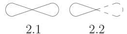
Figure 1: Two-line MIs. The solid and dashed lines correspond to propagators with mass $m_{t}$ and $M_{W}$, respectively.

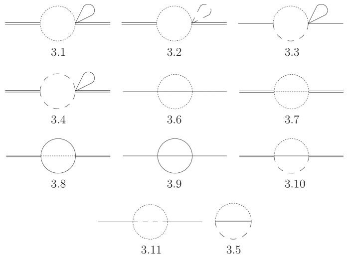
Figure 2: Three-line MIs. The solid, dashed and dotted lines correspond to propagators with mass $m_{t}$, $M_{W}$ and 0, respectively. Single external lines are on the mass shell with mass $m_{t}$ whereas double external line have mass $2m_{t}$. The topology denoted by 3.10 contains three master integrals, topology 3.11 contains two MIs.

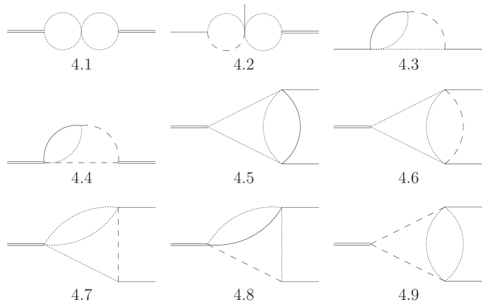
Figure 3: Four-line MIs. For the notation we refer to Fig. 2.

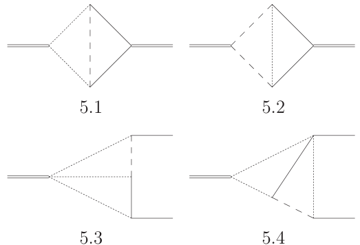
Figure 4: Five-line MIs. For the notation we refer to Fig. 2.

Some MIs factorize into one-loop integrals or contain only one dimensionful scale. Most of these integrals are available in the literature and can, e.g., be found in Refs. [35, 36, 37, 38, 8, 39].

As we will see in Section 4 a rapid convergence is observed if one considers an expansion of the matching coefficient in the quantity $z=M_{W}^{2}/m_{t}^{2}$. For this reason we evaluate the two-scale MIs in this limit. A promising method is based on differential equations (see Ref. [40] for a recent review) which provide the expansion in an automatic way once the initial conditions are specified. Let us as an example consider the five-line integral MI(5.2) (cf. Fig. 4) which fulfills the following differential equation

$$\frac{{\rm d}}{{\rm d}z}\,\text{MI}(5.2) = \frac{d-4}{z-1}\,\text{MI}(5.2)+\frac{3(z-2)(d-2)^{2}}{16m_{t}^{6}(d-3)(z-4)(z-1)^{2}z}\,\text{MI}(2.2)$$ (9)

$$\mbox{}-\frac{(d-2)}{4m_{t}^{4}(z-1)^{2}}\,\text{MI}(3.4)-\frac{(d-2)}{8m_{t}^{4}(z-1)^{2}}\,\text{MI}(3.5)$$

$$\mbox{}+\frac{(3d-8)(z-6)}{16m_{t}^{4}(z-4)(z-1)z}\,\text{MI}(3.10)$$

$$\mbox{}+\frac{(d-4)(z-9)(z+2)}{16m_{t}^{2}(d-3)(z-4)(z-1)z}\,\text{MI}(3.10.1)$$

$$\mbox{}-\frac{\left(z^{2}-z+6\right)}{4m_{t}^{2}(z-4)(z-1)^{2}z}\,\text{MI}(3.10.2)+\frac{(d-3)}{2m_{t}^{2}(z-1)^{2}}\,\text{MI}(4.4)\,.$$

MI(3.10.1) and MI(3.10.2) denote the MIs of the type 3.10 with a squared massless and top quark propagator, respectively. In order to solve this equation it is necessary to know the results of all integrals with less than five lines. With the help of the ansatz

$$\text{MI}(5.2)=\sum c_{ijk}\,\epsilon^{i}z^{j}(\ln z)^{k},$$ (10)

the differential equation can be expanded in $\epsilon$ and $z$. As a result it reduces to algebraic equations for the coefficients $c_{ijk}$. In every order in $\epsilon$ there is one constant $c_{ijk}$ which can not be determined with this procedure. It it obtained from the initial condition at $z=0$, which in the case of MI(5.2) can be found in Ref. [35]. In this way we have computed expansion terms up to order $z^{10}$ which can be found on the Mathematica file mentioned above. For illustration we present the first two expansion terms of MI(5.2) which read

$$\text{MI}(5.2)m_{t}^{2} = \frac{1}{4}\pi^{2}\ln 2-2\ln^{3}2-\frac{1}{3}\pi^{2}\ln 3+2\ln^{2}2\ln 3-\ln 2\ln^{2}3+\frac{\ln^{3}3}{3}$$ (11)

$$\mbox{}-\text{Li}_{3}(-2)+\frac{1}{2}\text{Li}_{3}\left(\frac{1}{4}\right)-2\text{Li}_{3}\left(\frac{2}{3}\right)+\text{Li}_{3}\left(\frac{3}{4}\right)+\frac{21\zeta(3)}{8}$$

$$\mbox{}-i\pi\left(\frac{\pi^{2}}{12}+\frac{1}{2}\ln^{2}2\right)-z\bigg{[}i\pi\left(\frac{1}{2}-\frac{1}{4}\ln 2+\frac{3}{4}\ln 3-\frac{3}{8}\ln z\right)$$

$$\mbox{}+\frac{3}{8}\ln 3\ln z-\frac{3\ln^{2}3}{8}+\frac{1}{4}\ln 2\ln 3-\frac{\ln^{2}2}{4}-\ln 2$$

$$\mbox{}+\frac{17\pi^{2}}{48}-\frac{1}{8}\text{Li}_{2}\left(\frac{3}{4}\right)\bigg{]}+{\cal O}(z^{2})\,.$$

Note that for some integrals the differential equation can be solved with the help of Harmonic Polylogarithms [41] which immediately leads to a closed result.

It is interesting to mention that for the integrals MI(4.3) and MI(4.4) no initial condition is needed in order to obtain all the coefficients in the ansatz. They are completely fixed by the corresponding differential equation and the solutions for the integrals of the subtopologies. For all other integrals initial conditions at $z=0$ are required. As already mentioned above most of them can be found in the literature or are quite simple to compute using standard techniques. However, we could not get analytic results for five coefficients in the $\epsilon$-expansion of the integrals MI(4.5), MI(4.8), MI(5.3) and MI(5.4) at $z=0$. We calculated these coefficients using the Mellin-Barnes method (see, e.g., Ref [42]) where we used the program packages AMBRE [43] and MB [44].

The Mellin-Barnes representation for a given integral is not unique. In particular it might happen that the convergence of the resulting numerical integration turns out to be good in one case whereas a poor convergence is observed in other cases. The crucial quantity in this respect is the asymptotic behaviour of the $\Gamma$ function for large imaginary part which is given by

$$\Gamma(a\pm ib)\stackrel{{\scriptstyle\tiny b\to\infty}}{{\simeq}}\sqrt{2\pi}e^{\pm i\frac{\pi}{4}(2a-1)}e^{\pm ib(\ln b-1)}e^{-\frac{b\pi}{2}}b^{a-\frac{1}{2}}\,,$$ (12)

where the first two exponential factors lead to oscillations. Let us discuss this in more detail for the Mellin-Barnes representation of the integral MI(4.5)

$$\text{MI}(4.5) = \left(\frac{e^{\gamma_{E}}\mu^{2}}{m_{t}^{2}}\right)^{2\epsilon}\int_{-i\infty}^{+i\infty}\frac{dz_{1}}{2\pi i}\int_{-i\infty}^{+i\infty}\frac{dz_{2}}{2\pi i}\,e^{i\pi(2\epsilon+z_{1})}4^{-2\epsilon-z_{2}}$$ (13)

$$\times\frac{\Gamma(1-\epsilon)\Gamma(-\epsilon-z_{1}+1)\Gamma(-z_{1})\left[\Gamma(-2\epsilon-z_{2}+1)\right]^{2}}{\Gamma(-3\epsilon-z_{1}+2)\Gamma(-2\epsilon-z_{1}+2)\Gamma(-4\epsilon-2z_{2}+2)}$$

$$\times\Gamma(-4\epsilon-z_{1}-z_{2}+2)\Gamma(z_{1}-z_{2})\Gamma(\epsilon+z_{2})\Gamma(2\epsilon+z_{2})\,,$$

where $\gamma_{E}=0.577216\dots$ and the contour of integration is chosen in such a way that the poles of the $\Gamma$ functions with $+z_{i}$ are separated from the poles of the $\Gamma$ functions with $-z_{i}$. Using the package MB we can expand the integrand in $\epsilon$. For the finite contribution this leads to a sum of an analytic part, a one-dimensional Mellin-Barnes integral and a two-dimensional one. The latter correspond to the integral in Eq. (13) for $\epsilon=0$. If we insert in this expression the asymptotic behaviour for the $\Gamma$ functions as given in Eq. (12) one can see that the integrand of the two-dimensional integral falls off exponentially, except for $\mbox{Im}(z_{2})=0,\mbox{Im}(z_{1})<0$. On this line the drop-off only shows a power-law behaviour which is dictated by the last factor of Eq. (12). In our particular case the drop-off turns out to be extremely slow for the integration contour chosen by MB which corresponds to $\mbox{Re}(z_{1})=-1/4$ and $\mbox{Re}(z_{2})=-1/2$. Thus it is hard to get an accurate result by the numerical integration since a highly oscillating functions has to be integrated. A closer look to the fall-off behaviour in Eq. (12) shows that it is possible to improve the drop-off for Im$(z_{1})\to-\infty$ by taking residues of the integrand in $z_{2}$ and thus shifting the integration contour for $z_{2}$ more and more to positive values for Re$(z_{2})$. In this way the integrand becomes well-behaved and can be integrated numerically with sufficiently high precision.

Let us mention that in the case of MI(4.5) there is an alternative possibility to improve the numerical properties of the Eq. (13): after the variable transformation $z_{2}\to z_{2}-2\epsilon$ MB chooses integration contours which lead to a rapid convergence of the numerical integration. We have checked that both approached lead to the same results and obtained 9 digits for the finite part of MI(4.5) in eleven minutes of CPU time.

The remaining three integrals show similar properties as MI(4.5). In all cases it is possible to end up with integrals which could be integrated numerically. Our results read

$$\text{MI}(4.5) = \left(\frac{\mu^{2}}{m_{t}^{2}}\right)^{2\epsilon}\bigg{[}\frac{1}{2\epsilon^{2}}+\frac{1}{\epsilon}\left(\frac{5}{2}-2\ln 2+i\pi\right)-4.81543683(7)$$

$$\mbox{}+4i\pi(1-\ln 2)\bigg{]}\,,$$

$$\text{MI}(4.8)|_{z=0} = \left(\frac{\mu^{2}}{m_{t}^{2}}\right)^{2\epsilon}\bigg{[}\frac{1}{2\epsilon^{2}}+\frac{1}{\epsilon}\left(\frac{5}{2}+i\pi\right)+\frac{19}{2}-\frac{23\pi^{2}}{24}-\frac{5\ln^{2}2}{2}-\frac{3\ln 3}{2}$$

$$\mbox{}+\frac{5}{2}\ln 2\ln 3-\frac{5}{4}\text{Li}_{2}\left(\frac{3}{4}\right)+\frac{i\pi}{2}(11-5\ln 2)-\epsilon\,16.690539(1)$$

$$\mbox{}-i\pi\epsilon\bigg{(}-\frac{45}{2}+\frac{35\pi^{2}}{24}+3\ln 2-\frac{21\ln^{2}2}{4}+6\ln 3+2\text{Li}_{2}(-2)$$

$$\mbox{}-4\text{Li}_{2}\left(\frac{1}{4}\right)\bigg{)}\bigg{]}\,,$$

$$m_{t}^{2}\,\text{MI}(5.3)|_{z=0} = 2.704628(4)-5.167709(4)i\,,$$

$$m_{t}^{2}\,\text{MI}(5.4)|_{z=0} = 2.70543(6)-1.91431(6)i\,.$$ (14)

The accuracy for the finite part of these integrals is sufficient to obtain the final result with four significant digits.

Note that contrary to the default settings of MB we do not use Vegas for the multidimensional numerical integrations. Instead we use Divonne which is available from the Cuba library [45]. For the integrals we have considered it leads to more accurate results using less CPU time.

We have performed an independent check of the initial conditions for all the MIs employing the method of sector decomposition. In particular we used program FIESTA [46].

4 The $\gamma t\bar{t}$ vertex

In this Section we discuss ${\cal O}(\alpha\alpha_{s})$ corrections to the $\gamma t\bar{t}$ vertex due to $W$ boson and gluon exchanges with incoming photon momentum at $q^{2}=4m_{t}^{2}$, the production threshold of top quark pairs. This leads to corrections to $h_{I,V}^{(1,1)}$ mediated by a virtual photon, i.e., to the first term of $h_{I,V}^{\rm tree}$ in Eq.(5). We denote by $\Gamma_{A}^{\,t}$ the contribution of the sum of all one-particle-irreducible diagrams to the $\gamma t\bar{t}$ vertex and parameterize the radiative corrections in the form

$$\hat{\Gamma}_{A}^{\,t}=Q_{t}+{\hat{\Gamma}}_{A}^{\,t,\,(0,1)}+{\hat{\Gamma}}_{A}^{\,t,\,(1,0)}+\hat{\Gamma}_{A}^{\,t,\,(1,1)}\,,$$ (15)

where the hat denotes renormalized quantities. Substituting $\hat{\Gamma}_{A}^{\,t}$ for the $Q_{t}$ in first line of Eq. (5) and retaining the relevant orders in the electroweak and strong couplings leads to the corrections to the helicity amplitudes, $h_{I,V}^{(0,1)},h_{I,V}^{(1,0)}$ and $h_{I,V}^{(1,1)}$. We further decompose $\hat{\Gamma}_{A}^{\,t}$ (and similarly the quantities on the right-hand side of Eq. (15)) according to the contributions from the Higgs, $Z$ and $W$ boson exchanges:

$$\hat{\Gamma}_{A}^{\,t}=\hat{\Gamma}_{A,H}^{\,t}+\hat{\Gamma}_{A,Z}^{\,t}+\hat{\Gamma}_{A,W}^{\,t}\,.$$ (16)

In this paper we compute the corrections up to order $\alpha\alpha_{s}$ to $\hat{\Gamma}_{A,W}^{t}$. The other two quantities have been computed in Ref. [8] where the matching coefficients $c_{v}^{\rm\,H,mix}$ and $c_{v}^{\rm\,Z,mix}$ have been introduced. We have the following relations

$$\hat{\Gamma}_{A,H}^{\,t,(1,1)}=\frac{\alpha\alpha_{s}}{\pi^{2}s_{w}^{2}}\,Q_{t}C_{F}\,c_{v}^{\rm\,H,mix},~{}~{}~{}\hat{\Gamma}_{A,Z}^{\,t,(1,1)}=\frac{\alpha\,\alpha_{s}}{\pi^{2}s_{w}^{2}}\,Q_{t}C_{F}\,c_{v}^{\rm\,Z,mix}\,.$$ (17)

In our calculation we adapt in the electroweak sector the t’Hooft-Feynman gauge, i.e. $\xi_{W}=1$, which guarantees a simple form of the $W$ boson propagator. Note that $\xi_{W}\not=1$ introduces an additional mass scale in our calculation which would lead to significantly more complicated integrals at two-loop order. We want to mention that our final result depends on $\xi_{W}$. This dependence only cancels out after including the self-energy and box contributions. There is no gauge parameter dependence in $\hat{\Gamma}_{A,H}^{\,t}$ which only occurs in the vertex and self-energy contributions. Also the vertex corrections involving the $Z$ boson ($\hat{\Gamma}_{A,Z}^{\,t}$) are independent of the corresponding gauge parameter.

Although the one-loop results are well-known, we start our discussion from this order since they enter the renormalization of the two-loop expressions.

4.1 One-loop corrections

The renormalized QCD contribution is given by

$$\hat{\Gamma}_{A}^{\,t,\,(0,1)} = \Gamma_{A}^{\,t,\,(0,1)}+Q_{t}\,Z_{2}^{(0,1)}\,,$$ (18)

where $Z_{2}$ is the onshell wave function renormalization for external top quarks. The expressions on the right-hand side of Eq. (18) are given by

$$\Gamma_{A}^{\,t,\,(0,1)} = Q_{t}\,\frac{\alpha_{s}C_{F}}{4\pi}\,\bigg{(}\frac{\mu^{2}}{m_{t}^{2}}\bigg{)}^{\epsilon}\,\bigg{[}\frac{3}{\epsilon}-4+\epsilon\,\bigg{(}8+\frac{\pi^{2}}{4}\bigg{)}\bigg{]},$$

$$Z_{2}^{(0,1)} = \frac{\alpha_{s}C_{F}}{4\pi}\,\bigg{(}\frac{\mu^{2}}{m_{t}^{2}}\bigg{)}^{\epsilon}\,\bigg{[}-\frac{3}{\epsilon}-4-\epsilon\,\bigg{(}8+\frac{\pi^{2}}{4}\bigg{)}\bigg{]},$$ (19)

where $C_{F}=4/3$. In Eq. (19) the ${\cal O}(\epsilon)$ terms are kept since they enter the finite part of the two-loop expression. For the renormalized vertex we have the relation

$$\hat{\Gamma}_{A}^{\,t,(0,1)} = Q_{t}\,c_{v}^{(1)}\,=\,-8\,Q_{t}\,\frac{\alpha_{s}C_{F}}{4\pi}\left(1+\epsilon\,L_{\mu}\right)+{\cal O}(\epsilon^{2})\,,$$ (20)

where $L_{\mu}=\ln\frac{\mu^{2}}{m_{t}^{2}}$. The one-loop formula for the electroweak corrections is given by

$${\hat{\Gamma}}_{A}^{\,t,\,(1,0)} = {\Gamma}_{A}^{t,\,(1,0)}+Q_{t}\,Z_{2}^{(1,0)}+T_{t}^{\,3}\,Z_{CT}^{(1,0)}\,,$$ (21)

where $Z_{CT}^{(1,0)}$ is a counterterm associated with $Z$-photon mixing at zero-momentum transfer [47] which reads

$$Z_{CT}^{(1,0)} = \frac{\alpha}{4\pi s_{w}^{2}}\left(-\frac{1}{\epsilon}-\ln\frac{\mu^{2}}{M_{W}^{2}}\right)+{\cal O}(\epsilon)\,.$$ (22)

As we will see later the ${\cal O}(\epsilon)$ term for $Z_{CT}^{(1,0)}$ is not needed. We present the remaining two ingredients as a series expansion of $z=M_{W}^{2}/m_{t}^{2}$, the exact formulae are collected in Appendix for convenience. The results for $Z_{2,W}^{(1,0)}$ reads

$$Z_{2,W}^{(1,0)} = \frac{\alpha}{4\pi s_{w}^{2}}\bigg{(}\frac{\mu^{2}}{m_{t}^{2}}\bigg{)}^{\epsilon}\,\bigg{\{}-\frac{1}{\epsilon}\bigg{(}\frac{1}{4}+\frac{1}{8z}\bigg{)}-\frac{i\pi}{8z}-\frac{L_{z}}{4}-\frac{i\pi}{2}-\frac{1}{4}-\left(\frac{L_{z}}{8}+\frac{i\pi}{8}+\frac{21}{16}\right)z$$ (23)

$$\mbox{}+\epsilon\,\bigg{[}\frac{7\pi^{2}}{96z}+\frac{L_{z}^{2}}{8}-\frac{L_{z}}{4}+\frac{5\pi^{2}}{16}-\frac{i\pi}{2}-\frac{3}{4}+\bigg{(}\frac{L_{z}^{2}}{16}+\frac{3L_{z}}{16}+\frac{\pi^{2}}{12}-\frac{9i\pi}{8}-\frac{27}{32}\bigg{)}z\bigg{]}\bigg{\}}$$

$$\mbox{}+{\cal O}(z^{2})\,,$$

and ${\Gamma}_{A,W}^{\,t,\,(1,0)}$ is given by

$${\Gamma}_{A,W}^{\,t,\,(1,0)} = \frac{\alpha}{4\pi s_{w}^{2}}\,Q_{b}\,\bigg{(}\frac{\mu^{2}}{m_{t}^{2}}\bigg{)}^{\epsilon}\,\bigg{\{}\frac{1}{\epsilon}\bigg{(}\frac{1}{8z}+\frac{1}{4}\bigg{)}+\frac{1}{z}\bigg{(}\frac{i\pi}{8}-\frac{2\ln{2}}{3}+\frac{1}{6}\bigg{)}$$ (24)

$$\mbox{}+\frac{L_{z}}{4}+\frac{i\,\pi}{2}-\frac{1}{12}-\frac{2\ln{2}}{3}+\bigg{(}\frac{L_{z}}{8}+\frac{i\,\pi}{8}+\frac{2\ln{2}}{3}+\frac{7}{48}\bigg{)}\,z$$

$$\mbox{}+\epsilon\,\bigg{[}\,-\frac{1}{z}\bigg{(}\frac{7\pi^{2}}{96}+\frac{i\pi\big{(}4\ln{2}-1\big{)}}{6}-\frac{2\ln{2}\big{(}3\ln{2}-5\big{)}}{9}-\frac{5}{18}\bigg{)}$$

$$\mbox{}-\frac{L_{z}^{2}}{8}+\frac{L_{z}}{4}-\frac{5\pi^{2}}{16}-\frac{i\pi\big{(}4\ln{2}-1\big{)}}{6}+\frac{2\ln{2}\,\big{(}3\ln{2}+1\big{)}}{9}+\frac{7}{36}$$

$$\mbox{}-\bigg{(}\frac{L_{z}^{2}}{16}+\frac{3L_{z}}{16}+\frac{2\ln{2}\big{(}3\ln{2}+1\big{)}}{9}+\frac{\pi^{2}}{12}-\frac{i\pi\big{(}16\ln{2}-1\big{)}}{24}-\frac{115}{288}\bigg{)}\,z\bigg{]}\bigg{\}}$$

$$\mbox{}+\frac{\alpha}{4\pi s_{w}^{2}}\,T_{t}^{\,3}\,\bigg{(}\frac{\mu^{2}}{m_{t}^{2}}\bigg{)}^{\epsilon}\,\bigg{\{}\,\frac{1}{\epsilon}\,\bigg{(}\frac{1}{4z}+\frac{3}{2}\bigg{)}+\frac{1}{z}\,\bigg{(}\frac{i\pi}{4}-\frac{2\ln{2}}{3}+\frac{2}{3}\bigg{)}$$

$$\mbox{}+\frac{3i\pi}{2}-3\ln{2}+3-\bigg{(}\frac{5L_{z}}{8}-\frac{15}{16}+\frac{5i\pi}{8}-\frac{7\ln{2}}{4}\bigg{)}\,z$$

$$\mbox{}+\epsilon\,\bigg{[}\,-\frac{1}{z}\,\bigg{(}\frac{7\pi^{2}}{48}+\frac{2i\pi\big{(}\ln{2}-1\big{)}}{3}-\frac{2\ln{2}\big{(}3\ln{2}-8\big{)}}{9}-\frac{13}{9}\bigg{)}$$

$$\mbox{}-\frac{7\pi^{2}}{8}-3i\pi\big{(}\ln{2}-1\big{)}+3\ln{2}\big{(}\ln{2}-2\big{)}+6$$

$$\mbox{}+\bigg{(}\frac{5L_{z}^{2}}{16}-\frac{11L_{z}}{16}+\frac{5\pi^{2}}{12}+\frac{i\pi\big{(}7\ln{2}+1\big{)}}{4}-\frac{7\ln^{2}{2}}{4}+\frac{39}{32}\bigg{)}\,z\bigg{]}\bigg{\}}$$

$$\mbox{}+{\cal O}(z^{2}),$$

where $L_{z}=\ln{z}$ and $\alpha=e^{2}/(4\pi)$ is the fine-structure constant in the Thomson limit. Again the ${\cal O}(\epsilon)$ terms are retained due to their relevance for the two-loop renormalization. Note that we keep the imaginary parts of both $\Gamma_{A,W}^{\,t,\,(0,1)}$ and $Z_{2,W}^{(0,1)}$. At one-loop order this only affects the finite part; at two loops also the pole parts are concerned (see below).

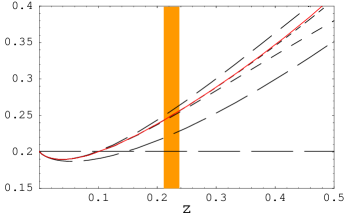
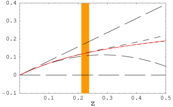
Figure 5: Electroweak one-loop corrections to the photon vertex $\hat{\Gamma}_{A,W}^{\,t,(1,0)}$ normalized to $\alpha/(4\pi s_{w}^{2})/z$ as a function of $z=M_{W}^{2}/m_{t}^{2}$, for real part (left panel) and imaginary part (right panel), respectively. The (black) dashed lines include successively higher orders in $z$ starting from $z^{0}$ (long dashes) to $z^{4}$ (short dashes) and the (red) solid line is the exact one-loop correction. The (orange) band marks the physical range of $z=(80.40~{}{\rm GeV}/m_{t})^{2}$ varying the top quark mass between $165$ and $175$ GeV.

We refrain from listing an analytical result for ${\hat{\Gamma}}_{A}^{\,t,\,(1,0)}$ but compare in Fig. 5 the approximated result to the exact one. The latter is represented by the (red) solid line whereas the dashed lines correspond to the expansions including successively higher orders in $z$. As one can see, the expression including the correction of order $z^{3}$ provides at the physical point $z\approx 0.23$ a perfect approximation to the exact result far below the per cent level. The approximated results are based on the following expressions

$$\hat{\Gamma}_{A,W}^{\,t,(1,0)} = \frac{\alpha}{4\pi s_{w}^{2}}\bigg{[}\,\frac{0.20}{z}+\big{(}0.48+0.79\,i+0.25\ln{z}\big{)}$$ (25)

$$\mbox{}+z\,\big{(}-0.0024-1.37\,i-0.44\,\ln{z}\big{)}+z^{2}\,\big{(}-0.072+1.39\,i+0.44\,\ln{z}\big{)}$$

$$\mbox{}+z^{3}\,\big{(}0.34-0.53\,i-0.17\,\ln{z}\big{)}+z^{4}\,\big{(}0.13+0.23\,i+0.074\,\ln{z}\big{)}\bigg{]}$$

$$\mbox{}+{\cal O}(z^{5})$$

$$= \bigg{[}2.48_{1/z}+0.25_{1}+0.39_{z}-0.095_{z^{2}}+0.017_{z^{3}}+0.00013_{z^{4}}$$

$$\mbox{}+i\,\big{(}2.11_{1}-0.80_{z}+0.18_{z^{2}}-0.015_{z^{3}}+0.0014_{z^{4}}\big{)}\,\bigg{]}\times 10^{-3}\,,$$

where the subscript in the last line indicate their order in the $z$ expansion and for the input parameters the following values have been used [48, 49]

$$\alpha_{s}=0.108\,,\qquad \alpha(M_{Z})=1/128.9\,, \qquad s_{w}^{2}=0.23\,,$$

$$M_{W}=80.40~{}\mbox{GeV}\,, m_{t}=172.4~{}\mbox{GeV}\,.$$ (26)

Note that in our numerical analysis we use $\alpha$ at high energy scale.

The corrections in Eq. (25) are dominated by the leading terms proportional to $m_{t}^{2}/M_{W}^{2}$. One observes a rapid convergence, so that the term of order $z^{3}$ can safely be neglected. Inserting the results in Eq. (15) the overall size of the electroweak corrections (from the diagrams involving a $W$ boson) amounts to about 0.5% and is unusually small. For comparison, we note that $\hat{\Gamma}_{A,Z}^{\,t,(1,0)}$ and $\hat{\Gamma}_{A,H}^{\,t,(1,0)}$ lead to corrections of 0.3% and 3.2% (for $M_{H}=120$ GeV), respectively. Let us mention that the one-loop QCD corrections provides a contribution “$-61\times 10^{-3}$” to the last line of Eq. (25) thus resulting in a 9% correction.

From Eq. (25) one obtains the corresponding corrections to the helicity amplitude as

$$\left[h_{I,V}^{(1,0)}\right]_{A,W} = Q_{e}\hat{\Gamma}_{A,W}^{\,t,(1,0)}\,,$$ (27)

which immediately leads to the correction to the cross section with the help of Eq. (1). Taking at tree-level both the photon and $Z$ exchange diagram we obtain a shift of 0.9% to $R(e^{+}e^{-}\rightarrow t\bar{t}X)$ due to the $W$ boson contribution to $\gamma t\bar{t}$ vertex at one-loop.

4.2 Two-loop order $\alpha\alpha_{s}$ renormalization

The renormalized $\gamma t\bar{t}$ vertex at order $\alpha\alpha_{s}$ is given by

$$\hat{\Gamma}_{A}^{\,t,\,(1,1)} = \Gamma_{A}^{\,t,\,(1,1)}+T_{t}^{\,3}\,Z_{CT}^{(1,1)}+Q_{t}\,Z_{2}^{(1,1)}$$ (28)

$$+\left(Z_{2}^{(1,0)}\,\Gamma_{A}^{\,t,\,(0,1)}+Z_{2}^{(0,1)}\,\Gamma_{A}^{\,t,\,(1,0)}\right)+\frac{T_{t}^{\,3}}{Q_{t}}\,Z_{CT}^{(1,0)}\,\hat{\Gamma}_{A}^{\,t,\,(0,1)},$$

where the first line corresponds to genuine two-loop diagrams and the second line consists of products of one-loop diagrams. For the latter we already listed all the relevant expressions in the previous Subsection. Note that in the last term the renormalized one-loop vertex appears and thus the ${\cal O}(\epsilon)$ term for $Z_{CT}^{(1,0)}$ is not needed.

Formula (28) takes only care of the renormalization of the external lines and the electric charge which means that the un-renormalized two-loop quantities in the first line are understood as the sum of the amputated two-loop diagrams and the corresponding counterterm diagrams for the top quark mass and the top quark Yukawa coupling. The latter are renormalized in the onshell scheme.

It is easy to see that for the two-loop counterterm we have $Z_{CT}^{(1,1)}=0$ since at one-loop order only bosonic and no fermionic diagrams contribute. The two-loop onshell wave function factor $Z_{2}^{(1,1)}$ has been computed in Ref. [50]. We confirmed the result by an independent calculation and added the imaginary part which is necessary in our framework. The result reads

$$Z_{2,W}^{(1,1)} = \frac{\alpha}{4\pi s_{w}^{2}}\frac{\alpha_{s}C_{F}}{4\pi}\,\bigg{\{}\,\frac{1}{\epsilon^{\,2}}\bigg{(}\frac{3}{4}+\frac{3}{4z}\bigg{)}+\frac{1}{\epsilon}\bigg{[}\,\frac{1}{z}\bigg{(}\frac{3{L_{\mu}}}{2}+\frac{7}{4}+\frac{3i\pi}{8}\bigg{)}+\frac{3{L_{\mu}}}{2}+\frac{3{L_{z}}}{4}$$ (29)

$$\mbox{}+\frac{17}{8}+\frac{3i\pi}{2}+\bigg{(}\frac{3{L_{z}}}{8}+\frac{63}{16}+\frac{3i\pi}{8}\bigg{)}z-\bigg{(}\frac{9\ln{z}}{4}-\frac{5}{4}+\frac{9i\pi}{4}\bigg{)}z^{2}\bigg{]}$$

$$\mbox{}+\frac{1}{z}\bigg{(}\frac{3L_{\mu}^{2}}{2}+\frac{\big{(}14+3i\pi\big{)}{L_{\mu}}}{4}+\frac{3\zeta(3)}{2}-\frac{i\pi^{3}}{6}-\frac{\pi^{2}}{4}+\frac{27i\pi}{8}+\frac{79}{16}\bigg{)}$$

$$\mbox{}+\frac{3L_{\mu}^{2}}{2}+\bigg{(}\frac{3{L_{z}}}{2}+\frac{17}{4}+3i\pi\bigg{)}{L_{\mu}}-\frac{3L_{z}^{2}}{8}+\frac{7{L_{z}}}{4}-3\zeta(3)+\frac{i\pi^{3}}{3}-\frac{\pi^{2}}{8}$$

$$\mbox{}+\frac{3i\pi}{2}-\frac{3}{16}+\bigg{[}\,\bigg{(}\frac{3{L_{z}}}{4}+\frac{3i\pi}{4}+\frac{63}{8}\bigg{)}{L_{\mu}}-\frac{3L_{z}^{2}}{16}-\frac{\big{(}1+28i\pi\big{)}{L_{z}}}{16}$$

$$\mbox{}-\frac{15\zeta(3)}{2}+\frac{5i\pi^{3}}{6}+\frac{5\pi^{2}}{6}-\frac{121i\pi}{24}+\frac{661}{32}\bigg{]}z+\bigg{[}\,\bigg{(}-\frac{9{L_{z}}}{2}+\frac{5}{2}-\frac{9i\pi}{2}\bigg{)}{L_{\mu}}$$

$$\mbox{}+\frac{9L_{z}^{2}}{8}+\bigg{(}\frac{1}{2}-\frac{5i\pi}{6}\bigg{)}\,L_{z}-\frac{317}{48}+\frac{547i\pi}{72}+\frac{79\pi^{2}}{36}-i\pi^{3}+9\zeta(3)\bigg{]}z^{2}\bigg{\}}$$

$$\mbox{}+{\cal O}(z^{3})\,,$$

where terms up to order $z^{2}$ have been included ($\zeta(3)=1.20205\cdots$).

In the following we provide the result for the un-renormalized vertex corrections where the finite part is given in numerical form. Our result reads

$$\Gamma_{A,W}^{\,t,(1,1)} = \frac{\alpha}{4\pi s_{w}^{2}}\frac{\alpha_{s}C_{F}}{4\pi}\,\bigg{\{}\frac{2}{\epsilon^{2}}+\frac{1}{\epsilon}\,\bigg{[}-\frac{1}{z}\,\bigg{(}\frac{1}{3}-\frac{i\pi}{4}+\frac{\ln{2}}{3}\bigg{)}+4{L_{\mu}}-\frac{L_{z}}{4}+\frac{7i\pi}{4}+\frac{5}{3}-\frac{23\ln{2}}{6}$$ (30)

$$\mbox{}-z\bigg{(}\,\frac{17{L_{z}}}{16}-\frac{47\ln{2}}{24}+\frac{17i\pi}{16}-\frac{121}{96}\bigg{)}-z^{2}\bigg{(}\,\frac{17{L_{z}}}{96}+\frac{185}{576}+\frac{17i\pi}{96}-\frac{65\ln{2}}{48}\bigg{)}\bigg{]}$$

$$\mbox{}+\frac{1}{z}\Big{(}\big{[}-2.66-3.79\big{]}-L_{\mu}\,\big{[}1.13-1.57i\big{]}\Big{)}+4.00\,L_{\mu}^{2}$$

$$\mbox{}+{L_{\mu}}\big{(}-0.50L_{Z}-\big{[}1.98-11.00i\big{]}\big{)}+0.13L_{z}^{2}+0.08L_{z}+\big{[}10.03-23.63i\big{]}$$

$$\mbox{}+z\,\bigg{[}L_{\mu}\,\Big{(}\big{[}5.24-6.68i\big{]}-2.13\,L_{z}\Big{)}+0.53\,L_{z}^{2}-L_{z}\,\big{[}0.77-7.76i\big{]}$$

$$\mbox{}-\big{[}11.84+5.62i\big{]}\bigg{]}+z^{2}\,\bigg{[}L_{\mu}\,\Big{(}\big{[}1.23-1.11i\big{]}-0.35\,L_{z}\Big{)}$$

$$\mbox{}+0.09\,L_{z}^{2}-L_{z}\,\big{[}3.80+1.16i\big{]}+\big{[}9.31+18.63i\big{]}\bigg{]}\bigg{\}}+{\cal O}(z^{3})\,.$$

Let us mention that in our calculation we allowed for a general QCD gauge parameter $\xi_{S}$ and used the independence of $\Gamma_{A}^{\,t,(1,1)}$ as a welcome check for the correctness of our result. Note that for the cancellation of $\xi_{S}$ it is important to include the counterterm diagram for the top quark mass. The remaining ingredients in Eq. (28) are individually $\xi_{S}$-independent. A further check of our calculation is based on a setup where we choose $M_{W}=0$ from the very beginning. This leads to significantly simpler expressions during the reduction to master integral, which is completely independent from the one for finite $M_{W}$.

4.3 ${\cal O}(\alpha\alpha_{s})$ corrections to the $\gamma t\bar{t}$ vertex

Inserting all ingredients into Eq. (28) leads to

$$\hat{\Gamma}_{A,W}^{\,t,(1,1)} = \frac{\alpha}{4\pi s_{w}^{2}}\frac{\alpha_{s}C_{F}}{4\pi}\,\bigg{[}\,\frac{1}{z}\,\bigg{(}-0.45-i\,2.06\bigg{)}+\bigg{(}6.34-i\,25.14-2.00\ln{z}\bigg{)}$$

$$\mbox{}+z\,\bigg{(}-6.27-i\,6.10+\big{(}2.16+i\,4.10\big{)}\,\ln{z}\bigg{)}$$

$$\mbox{}+z^{2}\,\bigg{(}13.50-i\,31.29-\big{(}4.53+i\,2.91\big{)}\,\ln{z}\bigg{)}$$

$$\mbox{}+z^{3}\,\bigg{(}-41.06-i\,5.55+\big{(}0.59+i\,13.10\big{)}\,\ln{z}\bigg{)}$$

$$\mbox{}+z^{4}\,\bigg{(}17.11-i\,9.99-\big{(}1.86+i\,5.36\big{)}\,\ln{z}\bigg{)}\bigg{]}+{\cal O}(z^{5})$$

$$= \bigg{[}\big{(}-0.64_{1/z}+2.89_{1}-0.64_{z}+0.30_{z^{2}}-0.13_{z^{3}}+0.014_{z^{4}}\big{)}$$

$$\mbox{}+i\,\big{(}-2.91_{1/z}-7.73_{1}-0.83_{z}-0.39_{z^{2}}-0.081_{z^{3}}-0.0013_{z^{4}}\big{)}\,\bigg{]}\times 10^{-4}\,.$$

In Fig. 6 we show the result for $\hat{\Gamma}_{A}^{\,t,(1,1)}$ including first five terms of the $z$ expansion. Taking the difference of two successive curves as a measure for the quality of the approximation we observe a rapid convergence at the physical point. Note that in contrast to the one-loop case the leading $1/z$ contribution is numerically not dominant.

Figure 6: Electroweak two-loop correction to the photon vertex $\hat{\Gamma}_{A,W}^{\,t,(1,0)}$ normalized to $(\alpha_{s}\alpha C_{F})/(16\pi^{2}s_{w}^{2})/z$ as a function of $z=M_{W}^{2}/m_{t}^{2}$, for real part (left panel) and imaginary part (right panel), respectively. The (black) long-dashed lines include successively higher orders in $z$ starting from $z^{0}$ (long dashes) to $z^{4}$ (short dashes) and the orange band is the physical range of $z$ (see Fig. 5).

In analogy to Eq. (27) we obtain for the correction to the helicity amplitude

$$\left[h_{I,V}^{(1,1)}\right]_{A,W} = Q_{e}\hat{\Gamma}_{A,W}^{\,t,(1,1)}\,,$$ (32)

which results in a correction of 0.1% to $R$.

Let us in the following briefly compare the new vertex corrections to the ones induced by a Higgs and $Z$ boson. Note that the latter two contain a non-trivial scale dependence which is canceled by the corresponding contribution from the effective theory [8]. Choosing $\mu=m_{t}$ one obtains [6, 8]

$$\hat{\Gamma}_{A,H}^{t,(1,0)}=21.1\times 10^{-3}~{}(10.6\times 10^{-3})~{}~{}~{}\mbox{for}~{}~{}M_{H}=120~{}(200)~{}{\rm GeV}\,,$$

$$\hat{\Gamma}_{A,W}^{t,(1,0)}=3.0\times 10^{-3}\,,$$

$$\hat{\Gamma}_{A,Z}^{t,(1,0)}=1.7\times 10^{-3}\,,$$

$$\hat{\Gamma}_{A,H}^{t,(1,1)}=-17.6\times 10^{-3}~{}(-6.6\times 10^{-3})~{}~{}~{}\mbox{for}~{}~{}M_{H}=120~{}(200)~{}{\rm GeV}\,,$$

$$\hat{\Gamma}_{A,W}^{t,(1,1)}=0.2\times 10^{-3}\,,$$

$$\hat{\Gamma}_{A,Z}^{t,(1,1)}=-1.0\times 10^{-3}\,.$$ (33)

One observes quite small corrections from the $W$ and $Z$ boson induced contributions. From Eq. (33) one can read off that relatively big one-loop effects are obtained for light Higgs boson masses. However, there is a strong cancellation between the one- and two-loop terms resulting in corrections which have the same size as the sum of the one- and two-loop contributions of the $W$ and $Z$ boson diagrams. In general moderate effects are observed suggesting that in the electroweak sector perturbation theory works well, which is in contrast to the pure QCD corrections.

Let us at this point comment on the imaginary parts contained in Eqs. (25) and (LABEL:eq::num2l) which are not taken into account in the numerical estimates for the corrections to $R$ presented above. As we mentioned previously, “${\rm Im}$” in Eq. (1) applies to the imaginary part which corresponds to the $t\bar{t}X$ final state or experimentally indistinguishable cuts involving bottom quarks and $W$ bosons. Thus, it is necessary to separate imaginary parts arising from cutting, e.g., two $W$ boson or two $b$ quark lines from the $t\bar{t}X$ cuts in order to make a phenomenological prediction. This requires a dedicated analysis in the loop calculation, which is beyond the scope of this paper (see, e.g., Ref. [11]).

5 Conclusions and outlook

Mixed two-loop electroweak/QCD corrections to the $\gamma t\bar{t}$ vertex due to $W$ boson and gluon exchange have been computed. The new contribution completes the order $\alpha\alpha_{s}$ corrections to the $\gamma t\bar{t}$ vertex. The numerical evaluation leads to a shift of 0.1% in the threshold production cross section of top quark pairs at $e^{+}e^{-}$ colliders which is small as compared to the aimed 3% uncertainty for the theory predictions. Nevertheless, it is remarkable that in the sum of the order $\alpha$ and order $\alpha\alpha_{s}$ correction terms the sizeable one-loop contribution from the Higgs boson induced diagrams is screened resulting in numerical values comparable to the $W$ and $Z$ boson contributions.

We want to mention that the corrections evaluated in this paper can be taken over in a straightforward way to the vector coupling of the $Zt\bar{t}$ vertex. Note, that the axial-vector contribution is suppressed at threshold and thus one-loop corrections are sufficient.

The only missing building block in order to complete the order $\alpha\alpha_{s}$ corrections to the process $e^{+}e^{-}\to t\bar{t}$ are the two-loop box diagrams. They are technically more involved and are thus postponed to future work.

Acknowledgements

We would like to thank J.H. Kühn for helpful discussions and A. Smirnov and M. Tentyukov for providing the package FIESTA prior to its publication. Y.K. thanks N. Zerf for comparing the electroweak one-loop corrections and Y. Sumino for discussions about the implementation of the sector decomposition method within Mathematica. D.S. acknowledges technical support by T. Hahn concerning to the Cuba library. This work is supported by the DFG Sonderforschungsbereich/Transregio 9 “Computergestützte Theoretische Teilchenphysik”.

Appendix: Exact result for $\Gamma_{A,W}^{\,t,(1,0)}$

Keeping the full dependence on $\epsilon$ the exact one-loop result for the $\gamma t\bar{t}$ vertex due to the $W$ boson exchange reads (for massless bottom quarks)

$$\Gamma_{A,W}^{\,t,(1,0)} = \frac{\alpha}{4\pi s_{w}^{2}}\bigg{(}\frac{1}{-3+2\,\epsilon}\bigg{)}\bigg{[}\big{(}Q_{b}+2T_{t}^{3}\big{)}\big{(}1+2(1-\epsilon)z\big{)}\frac{A_{0}^{(\epsilon)}\big{(}M_{W}^{2}\big{)}}{8M_{W}^{2}}$$ (34)

$$\mbox{}+\big{(}Q_{b}\,(5+z-4\epsilon)+2T_{t}^{3}\,(1+z)\big{)}\frac{(1-z)\big{(}1+2(1-\epsilon)z\big{)}}{8z(1+z)}B_{0}^{(\epsilon)}(m_{t}^{2},M_{W}^{2},0)$$

$$\mbox{}-Q_{b}\frac{(1+2(1-\epsilon)z)(1-\epsilon)}{z(1+z)}B_{0}^{(\epsilon)}(4m_{t}^{2},0,0)$$

$$\mbox{}-T_{t}^{3}\,\bigg{(}\frac{1}{z}+5-4\epsilon\bigg{)}\,B_{0}^{(\epsilon)}(4m_{t}^{2},M_{W}^{2},M_{W}^{2})\bigg{]},$$

where $Q_{b}=-1/3$ is bottom quark electric charge normalized to the one of positron. The corresponding contribution to the wave function renormalization constant reads

$$Z_{2}^{(1,0)} = \frac{\alpha}{4\pi s_{w}^{2}}\bigg{[}\big{(}1+2\,(1-\epsilon)\,z\big{)}\frac{A_{0}^{(\epsilon)}\big{(}M_{W}^{2}\big{)}}{8M_{W}^{2}}-\frac{(1+z)\big{(}1+2\,(1-\epsilon)\,z\big{)}}{8z}B_{0}^{(\epsilon)}(m_{t}^{2},M_{W}^{2},0)$$ (35)

$$\mbox{}-\frac{(1-z)\big{(}1+2\,(1-\epsilon)\,z\big{)}}{4z}\,\big{\{}m_{t}^{2}\frac{\partial}{\partial m_{t}^{2}}B_{0}^{(\epsilon)}(m_{t}^{2},M_{W}^{2},0)\big{\}}\bigg{]}.$$

The loop-functions $A_{0}^{(\epsilon)}$ and $B_{0}^{(\epsilon)}$ are given by

$$A_{0}^{(\epsilon)}(M_{W}^{2})/M_{W}^{2} = -\bigg{(}\frac{e^{\gamma_{E}}\mu^{2}}{M_{W}^{2}}\bigg{)}^{\epsilon}\,\Gamma(-1+\epsilon),$$ (36)

$$B_{0}^{(\epsilon)}(4m_{t}^{2},0,0) = \bigg{(}-\frac{e^{\gamma_{E}}\mu^{2}}{m_{t}^{2}}\bigg{)}^{\epsilon}\,\frac{\sqrt{\pi}\,\Gamma(\epsilon)\,\Gamma(1-\epsilon)}{2\,\Gamma(\frac{3}{2}-\epsilon)},$$ (37)

$$B_{0}^{(\epsilon)}(m_{t}^{2},M_{W}^{2},0) = \bigg{(}\frac{e^{\gamma_{E}}\mu^{2}}{m_{t}^{2}}\bigg{)}^{\epsilon}\bigg{(}-1+\frac{M_{W}^{2}}{m_{t}^{2}}\bigg{)}^{-\epsilon}\,\frac{\Gamma(\epsilon)}{1-\epsilon}\,$$ (38)

$$\times{\,{}_{2}F_{1}}\bigg{(}\epsilon,1-\epsilon,2-\epsilon;\,1/(1-M_{W}^{2}/m_{t}^{2})\bigg{)},$$

$$B_{0}^{(\epsilon)}(4m_{t}^{2},M_{W}^{2},M_{W}^{2}) = \frac{1}{2(1-\epsilon)}\,\bigg{(}\frac{e^{\gamma_{E}}\mu^{2}}{2M_{W}^{2}}\bigg{)}^{\epsilon}\,\Gamma(\epsilon)\,$$

$$\times\bigg{[}\bigg{(}1-\frac{1}{\sqrt{1-\frac{M_{W}^{2}}{m_{t}^{2}}}}\bigg{)}^{\epsilon}\bigg{(}1+\sqrt{1-\frac{M_{W}^{2}}{m_{t}^{2}}}\bigg{)}{{}_{2}F_{1}\bigg{(}1-\epsilon,\epsilon,2-\epsilon;\frac{1}{2}\bigg{(}1+\frac{1}{\sqrt{1-\frac{M_{W}^{2}}{m_{t}^{2}}}}\bigg{)}\bigg{)}}$$

$$~{}~{}+\bigg{(}1+\frac{1}{\sqrt{1-\frac{M_{W}^{2}}{m_{t}^{2}}}}\bigg{)}^{\epsilon}\bigg{(}1-\sqrt{1-\frac{M_{W}^{2}}{m_{t}^{2}}}\bigg{)}{{}_{2}F_{1}\bigg{(}1-\epsilon,\epsilon,2-\epsilon;\frac{1}{2}\bigg{(}1-\frac{1}{\sqrt{1-\frac{M_{W}^{2}}{m_{t}^{2}}}}\bigg{)}\bigg{)}}\bigg{]},$$

where an analytic continuation by $(m_{t}^{2}+i0)$ is understood. Expansions with respect to $\epsilon$ of the Gauss-hypergeometric functions ${{}_{2}F_{1}}$ around integer values is well known in the literature (see, e.g., Ref. [38] or the package HypExp [51]).

References

• [1] M. Martinez and R. Miquel, Eur. Phys. J.  C 27 (2003) 49 [arXiv:hep-ph/0207315].
• [2] A. H. Hoang, Acta Phys. Polon.  B 34 (2003) 4491 [arXiv:hep-ph/0310301].
• [3] A. Pineda and A. Signer, Nucl. Phys.  B 762 (2007) 67 [arXiv:hep-ph/0607239].
• [4] M. Beneke, Y. Kiyo and K. Schuller, arXiv:0801.3464 [hep-ph].
• [5] M. Beneke, Y. Kiyo and A. A. Penin, Phys. Lett.  B 653 (2007) 53 [arXiv:0706.2733 [hep-ph]]; M. Beneke and Y. Kiyo, arXiv:0804.4004 [hep-ph] (Phys. Lett. B in press).
• [6] R. J. Guth and J. H. Kühn, Nucl. Phys.  B 368 (1992) 38.
• [7] A. H. Hoang and C. J. Reisser, Phys. Rev.  D 74 (2006) 034002 [arXiv:hep-ph/0604104].
• [8] D. Eiras and M. Steinhauser, Nucl. Phys.  B 757 (2006) 197 [arXiv:hep-ph/0605227].
• [9] B. A. Kniehl, Nucl. Phys.  B 347 (1990) 86.
• [10] A. Djouadi and P. Gambino, Phys. Rev.  D 49 (1994) 3499 [Erratum-ibid.  D 53 (1996) 4111] [arXiv:hep-ph/9309298].
• [11] A. H. Hoang and C. J. Reisser, Phys. Rev.  D 71 (2005) 074022 [arXiv:hep-ph/0412258].
• [12] G. T. Bodwin, E. Braaten and G. P. Lepage, Phys. Rev.  D 51 (1995) 1125 [Erratum-ibid.  D 55 (1997) 5853] [arXiv:hep-ph/9407339].
• [13] M. E. Luke and M. J. Savage, Phys. Rev.  D 57 (1998) 413 [arXiv:hep-ph/9707313].
• [14] M. Beneke and V. A. Smirnov, Nucl. Phys.  B 522 (1998) 321 [arXiv:hep-ph/9711391].
• [15] A. Pineda and J. Soto, Nucl. Phys. Proc. Suppl.  64 (1998) 428 [arXiv:hep-ph/9707481].
• [16] N. Brambilla, A. Pineda, J. Soto and A. Vairo, Nucl. Phys.  B 566 (2000) 275 [arXiv:hep-ph/9907240].
• [17] B. A. Kniehl, A. A. Penin, V. A. Smirnov and M. Steinhauser, Nucl. Phys.  B 635 (2002) 357 [arXiv:hep-ph/0203166].
• [18] A. V. Smirnov, V. A. Smirnov and M. Steinhauser, arXiv:0809.1927 [hep-ph] (Phys. Lett. B in press).
• [19] V. S. Fadin and V. A. Khoze, JETP Lett.  46 (1987) 525 [Pisma Zh. Eksp. Teor. Fiz.  46 (1987) 417].
• [20] A. A. Penin and A. A. Pivovarov, Phys. Atom. Nucl.  64 (2001) 275 [Yad. Fiz.  64 (2001) 323] [arXiv:hep-ph/9904278].
• [21] B. A. Kniehl and A. A. Penin, Nucl. Phys.  B 563 (1999) 200 [arXiv:hep-ph/9907489].
• [22] A. V. Manohar and I. W. Stewart, Phys. Rev.  D 63 (2001) 054004 [arXiv:hep-ph/0003107].
• [23] B. A. Kniehl, A. A. Penin, M. Steinhauser and V. A. Smirnov, Phys. Rev. Lett.  90 (2003) 212001 [arXiv:hep-ph/0210161]; Phys. Rev.  Lett.  91 (2003) 139903, Erratum.
• [24] A. H. Hoang, Phys. Rev.  D 69 (2004) 034009 [arXiv:hep-ph/0307376].
• [25] A. A. Penin, V. A. Smirnov and M. Steinhauser, Nucl. Phys.  B 716 (2005) 303 [arXiv:hep-ph/0501042].
• [26] A. Czarnecki and K. Melnikov, Phys. Rev. Lett.  80 (1998) 2531 [arXiv:hep-ph/9712222].
• [27] M. Beneke, A. Signer and V. A. Smirnov, Phys. Rev. Lett.  80 (1998) 2535 [arXiv:hep-ph/9712302].
• [28] P. Marquard, J. H. Piclum, D. Seidel and M. Steinhauser, Nucl. Phys.  B 758 (2006) 144 [arXiv:hep-ph/0607168].
• [29] P. Nogueira, J. Comput. Phys.  105 (1993) 279.
• [30] R. Harlander, T. Seidensticker and M. Steinhauser, Phys. Lett. B 426 (1998) 125 [hep-ph/9712228].
• [31] T. Seidensticker, hep-ph/9905298.
• [32] P. Marquard and D. Seidel, unpublished.
• [33] S. Laporta and E. Remiddi, Phys. Lett. B 379 (1996) 283 [arXiv:hep-ph/9602417].
• [34] S. Laporta, Int. J. Mod. Phys.  A 15 (2000) 5087 [arXiv:hep-ph/0102033].
• [35] R. Scharf and J. B. Tausk, Nucl. Phys.  B 412 (1994) 523.
• [36] J. Fleischer, F. Jegerlehner, O. V. Tarasov and O. L. Veretin, Nucl. Phys.  B 539 (1999) 671 [Erratum-ibid.  B 571 (2000) 511] [arXiv:hep-ph/9803493].
• [37] D. Seidel, Phys. Rev.  D 70 (2004) 094038 [arXiv:hep-ph/0403185].
• [38] M. Y. Kalmykov, JHEP 0604 (2006) 056 [arXiv:hep-th/0602028].
• [39] J. H. Piclum, “Heavy quark threshold dynamics in higher order,” Dissertation, Hamburg University, 2007.
• [40] M. Argeri and P. Mastrolia, Int. J. Mod. Phys.  A 22 (2007) 4375 [arXiv:0707.4037 [hep-ph]].
• [41] E. Remiddi and J. A. M. Vermaseren, Int. J. Mod. Phys.  A 15 (2000) 725 [arXiv:hep-ph/9905237].
• [42] V. A. Smirnov, “Evaluating Feynman Integrals,” Springer Tracts Mod. Phys.  211 (2004) 1.
• [43] J. Gluza, K. Kajda and T. Riemann, Comput. Phys. Commun.  177 (2007) 879 [arXiv:0704.2423 [hep-ph]].
• [44] M. Czakon, Comput. Phys. Commun.  175 (2006) 559 [arXiv:hep-ph/0511200].
• [45] T. Hahn, Comput. Phys. Commun.  168 (2005) 78 [arXiv:hep-ph/0404043].
• [46] A. V. Smirnov and M. N. Tentyukov, arXiv:0807.4129 [hep-ph].
• [47] A. Denner, Fortsch. Phys.  41 (1993) 307 [arXiv:0709.1075 [hep-ph]].
• [48] LEP Electroweak Working Group (LEP EWWG), see
http://lepewwg.web.cern.ch/LEPEWWG
• [49] Tevatron Electroweak Working Group and CDF and D0 Collaboration, arXiv:0808.1089 [hep-ex].
• [50] D. Eiras and M. Steinhauser, JHEP 0602 (2006) 010 [arXiv:hep-ph/0512099].
• [51] T. Huber and D. Maitre, Comput. Phys. Commun.  178 (2008) 755 [arXiv:0708.2443 [hep-ph]].