Towards active microfluidics: Interface turbulence in thin liquid films with floating molecular machines

Abstract

Thin liquid films with floating active protein machines are considered. Cyclic mechanical motions within the machines, representing microscopic swimmers, lead to molecular propulsion forces applied to the air-liquid interface. We show that, when the rate of energy supply to the machines exceeds a threshold, the flat interface becomes linearly unstable. As the result of this instability, the regime of interface turbulence, characterized by irregular traveling waves and propagating machine clusters, is established. Numerical investigations of this nonlinear regime are performed. Conditions for the experimental observation of the instability are discussed.

I Introduction

Molecular machines are protein molecules which can transform chemical energy into ordered internal mechanical motions. The classical examples of such machines are molecular motors kinesin and myosin, where internal mechanical motions are used to transport cargo along microtubules and filaments. Many enzymes operate as machines, using internal conformational motions to facilitate chemical reactions. Other kinds of machines, operating as ion pumps or involved in genetic processes, are also known. Moreover, artificial nonequilibrium nanodevices, similar to protein machines, are being developed kay2007 .

The cycle of a protein machine is typically powered by chemical energy supplied with an ATP molecule. When an ATP molecule binds to a protein machine, the initial protein-ATP complex is out of equilibrium and the process of ordered conformational relaxation of this complex towards its equilibrium state starts. When this state is reached, ATP is converted into ADP and this product molecule leaves the complex. The emerging free protein molecule is out of equilibrium and another conformational relaxation process, returning the free protein to its original equilibrium state begins. Thus, the cycle consists of two conformational motions. It is important to note that the forward and back conformational motions inside each cycle do not coincide - they correspond to relaxation processes in two different physical objects, i.e. the free protein and the protein-ATP complex togashi2007 .

Recently, much attention has been attracted to microscale swimmers operating at low Reynolds numbers. Generally, it can be shown that any physical object, cyclically changing its shape in such a way that the internal forward and back motions are different, propels itself through the liquid purcell1976 ; shapere1987 . Elementary models of such swimmers, constructed by joining together mobile links purcell1976 ; becker2003 or by connecting a few spheres by several actively deformable links najafi2004 ; earl2007 ; golestanian2008 , have been considered. Typically, the concept of molecular swimmers is applied to explain active motion of bacteria and other microorganisms. However, individual macromolecules that operate actively as machines are also capable of self-motion kay2007 ; golestanian2008prl

If a swimmer is attached to some support, preventing its translational motion, it exhibits force acting on the mechanical support. The generated force is equal to the stall force which needs to be applied to a swimmer to prevent its translational motion. When many swimmers are attached to a distributed support, their collective operation produces mechanical pressure acting on the support. This situation is, for example, encountered for molecular machines representing active protein inclusions (such as ion pumps) in biological membranes. It has been shown that the combined effects of the mechanical forces generated by the machines and their lateral motions inside the membrane can lead to membrane instabilities Ramaswamy2000 .

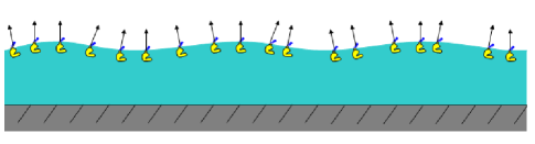
Figure 1: (Color online) Sketch of a thin film with floating molecular machines generating propulsion forces.

The aim of this paper is to investigate a different situation involving molecular machine populations. We consider hypothetical machines which are floating on top of a thin liquid layer and thus represent active surfactants (Fig.1). Because the considered surfactant molecules are microswimmers, they generate local pressure applied to the liquid-air interface and proportional to their local concentration. Additionally, they are subject to surface diffusion and, as surfactants, also modify local surface tension. Our main analytical result, supported by numerical simulations, is that, if the surface density of machines is sufficiently high and if the rate of supply of chemical energy to the machine population exceeds a threshold, the equilibrium flat interface becomes unstable and hydrodynamical flows inside the liquid layer spontaneously develop. This instability is accompanied by spatial redistribution of floating machines and their collective motions over the surface. It leads to the emergence of a special kind of surface turbulence. Such phenomena can provide the basis for active microfluidics, where hydrodynamical motions in liquid layers are induced and controlled by molecular machines located at the surface.

The next two sections are devoted to the derivation and the stability analysis of a model of such molecular swimmers attached to the surface of a thin liquid film. A collection of numerical results is presented in section IV. Finally, a model and numerical results are discussed, and some estimates of the forces of such molecules are given. The possible experimental realization is also discussed.

II Formulation of the Model

Population of identical molecular machines floating on the surface of a thin liquid film will be considered. These machines perform cycles of conformational changes (with a characteristic time $t_{c}$) enabled by the supply of energy through ATP molecules present in the liquid. We are interested in macroscopic collective effects and do not specify the details of machine operation. It will be assumed that, on the average, each machine generates the force which is applied to the air-liquid interface. This average force acts along the normal direction (the forces in the lateral direction vanish after averaging because of the rotational diffusion). Each machine cycle is initiated by binding of an ATP molecule and the average force is proportional to the cycle frequency. Assuming that binding of ATP molecules follows the Michaelis-Menten law, the average force per machine molecule is

$$f=f_{0}\frac{[ATP]}{K_{ATP}+[ATP]}.$$ (1)

Here, $f_{0}$ is the maximal force under the ATP saturation conditions, $\left[ATP\right]$ denotes the ATP concentration in the liquid, and $K_{ATP}$ is the characteristic concentration at which saturation begins.

Because of the cycles, the floating machines produce additional pressure acting on the air-liquid interface. This pressure $p_{m}$ is proportional to the local surface concentration of the machines and the average force generated by an individual machine, i.e. $p_{m}=f_{m}c$, where $f_{m}$ is the force per Mol of molecules ($f_{m}=fN_{A}$ where $N_{A}$ is the Avogadro number). Note that the machines are still sufficiently well separated one from another and possible synchronization effects of their cycles (cf. casagrande2007 ) are therefore neglected.

Before proceeding to the detailed formulation of the model, we want to outline the origin of the expected surface instability. Suppose that the average force, generated by machines is directed upwards and therefore the machines are pulling the liquid up in the vertical direction (Fig. 2A). If machine concentration is increased in some region, the pulling pressure is higher in this region, inducing local rise in the liquid film thickness. This however leads to lateral hydrodynamical flows which are directed inwards and bring even more machines into the region. As a result, the positive feedback, responsible for the instability, is established. Note that surface diffusion of floating machines and capillary forces are acting in the opposite direction, suppressing the instability. Thus, it is observed only if the average force $f$ generated by a machine is large enough, setting a threshold in terms of the energy supply rate (i.e., of the ATP concentration in the solution). The instability is not possible when the force is downwards directed, thus inducing local depressions of the liquid layer (Fig. 2B), Then, in contrast to the previous case, hydrodynamical flows remove machines from the depression, restoring the equilibrium flat film.

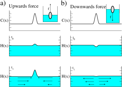
Figure 2: (Color online) Mechanisms of (a) instability development for upwards directed propulsion forces, and of (b) instability damping for downwards directed propulsion forces.

Temporal evolution of the surface concentration field $c$ is described by the equation :

$$\partial_{t}c+\vec{\nabla}\left(\vec{u}c\right)=d\nabla^{2}c,$$ (2)

where $\vec{u}$ is the lateral fluid velocity and $d$ is the surface diffusion.

Floating proteins represent surfactants and reduce the surface tension of the interfaces (see beverung1999 ). To take this effect into account, we assume that the surface tension coefficient $\sigma$ decreases linearly with the machine concentration,

$$\sigma=\sigma_{0}-\sigma_{c}c\text{.}$$ (3)

Hydrodynamical flows, induced by the gradients in machine concentration, should be further considered. We assume that the liquid layer is so thin that the lubrication approximation, typically employed in microfluidics oron1997 , is justified. As shown in Appendix A, the evolution equation for the local hight $h$ of the interface has the form

$$\partial_{t}h=\frac{1}{\mu}\vec{\nabla}\left(\frac{h^{3}}{3}\vec{\nabla}p-\frac{h^{2}}{2}\vec{\nabla}\sigma\right),$$ (4)

where the local pressure is $p=-\sigma\nabla^{2}h-p_{m}$ and $\mu$ is the viscosity of the fluid. Determining the lateral flow velocity at the interface (see Appendix A) and substituting it into the evolution equation for the surface concentration, a closed set of two partial differential equations is obtained.

Explicitly, the considered dynamics of thin films with active surfactants is described by equations:

$$\partial_{t}h =-\frac{1}{\mu}\vec{\nabla}\left[\frac{h^{3}}{3}\left(\vec{\nabla}\left(\sigma_{0}\nabla^{2}h-\sigma_{c}c\nabla^{2}h+f_{m}c\right)\right)\right]$$

$$+\frac{1}{\mu}\sigma_{c}\vec{\nabla}\left(\frac{h^{2}}{2}\vec{\nabla}c\right),$$ (5)

$$\partial_{t}c =-\frac{1}{\mu}\vec{\nabla}\left[c\frac{h^{2}}{2}\vec{\nabla}\left(\sigma_{0}\nabla^{2}h-\sigma_{c}c\nabla^{2}h+f_{m}c\right)\right]$$

$$+\frac{1}{\mu}\sigma_{c}\vec{\nabla}\left(ch\vec{\nabla}c\right)+d\nabla^{2}c.$$ (6)

Note that we have assumed that the active surfactant is insoluble oron1997 ; dewit1994 .

For subsequent analysis, it is convenient to write these equations in the dimensionless form. The (equilibrium) liquid layer thickness $h_{0}$ will be used as the length unit, time will be measured in units of $\mu h_{0}/\sigma_{0}$, and local concentration $c$ in units of the equilibrium machine concentration $c_{0}$. Changing the variables as $T=(\sigma_{0}/\mu h_{0})t$, $H=h/h_{0}$, $X=x/h_{0}$ and $C=c/c_{0}$, we obtain

$$\partial_{T}H =-\frac{1}{3}\vec{\nabla}\left(H^{3}\vec{\nabla}\left[\left(1-AC\right)(\nabla^{2}H)+BC\right]\right)$$

$$+\frac{A}{2}\vec{\nabla}\left(H^{2}(\vec{\nabla}C)\right),$$ (7)

$$\partial_{T}C =-\frac{1}{2}\vec{\nabla}\left[CH^{2}\vec{\nabla}\left(\left(1-AC\right)(\nabla^{2}H)+BC\right)\right]$$

$$+A\vec{\nabla}\left[CH\vec{\nabla}C\right]+D\nabla^{2}C.$$ (8)

The new model equations include only three dimensionless parameters

$$A=\frac{\sigma_{c}c_{0}}{\sigma_{0}},\qquad B=\frac{f_{m}c_{0}h_{0}}{\sigma_{0}},\qquad D=\frac{d\mu}{\sigma_{0}h_{0}}.$$

The parameter $A$ specifies the characteristic strength of floating machines as the surfactant species (decreasing the local surface tension of the interface). The parameter $B$ specifies the magnitude of the pressure generated by the cycling molecular machines; it is controlled by the rate of energy supply to the system. Finally, $D$ is the dimensionless diffusion coefficient of floating machines.

Comparing the last terms in equation (8), we notice that spreading of floating machines, induced by changes in the surface tension, has the same functional form as surface diffusion. If relative variations of the film thickness and machine concentration are small ($H\sim C\sim 1$), the effective diffusion coefficient of this process is $A$. Our estimates below in Sect. V indicate that the genuine diffusion constant $D$ of floating machines is typically much smaller than the effective diffusion constant $A$. Having this in mind, we retain the terms including the coefficient $D$ in our analytical investigations, but put $D=0$ when numerical simulations of the model are performed. Results with non-zero diffusion coefficient have been also obtained but they are very close to the results with $D=0$.

As shown in Appendix A, the dimensionless horizontal ($\vec{U}$) and vertical ($W$) velocities of the liquid film at hight $Z=z/h_{0}$ and horizontal spatial location $X$ can be found as

$$\vec{U}(X,Z)=-A\vec{\nabla}CZ$$ (9)

$$+\frac{1}{2}\left(B\vec{\nabla}C+\vec{\nabla}\left(\left(1-AC\right)\nabla^{2}H\right)\right)(2HZ-Z^{2}),$$

$$W(X,Z)=-\frac{1}{2}A\nabla^{2}CZ^{2}$$ (10)

$$+\frac{1}{2}\left(HZ^{2}-\frac{Z^{3}}{3}\right)\nabla^{2}\left(BC+\left(1-AC\right)\nabla^{2}H\right)$$

$$-Z^{2}\vec{\nabla}H\left((B-A\nabla^{2}H)\vec{\nabla}C+(1-AC)\vec{\nabla}\nabla^{2}H\right)$$

when the fields $C$ and $H$ are known. Both velocities vanish at the bottom of the liquid film, at $Z=0$, because of the no-penetration and no-slip boundary conditions imposed there.

III Linear stability analysis

The model always has the stationary uniform state $C=H=1$. To perform the linear stability analysis of this state, small perturbations $H=1+\Delta H$ $\exp(iKX+ST)$ and $C=1+\Delta C$ $\exp(iKX+ST)$ in the form of plane waves with the wavenumber $K$ are introduced. Linearizing evolution equations with respect to small perturbations $\Delta H$ and $\Delta C$ and solving the linearized equations, growth rates $S=S(K)$ of such perturbations are obtained,

$$S(K) =-\frac{1}{2}\left(A-\frac{B}{2}+D\right)K^{2}-\frac{1}{6}(1-A)K^{4}$$ (11)

$$\pm\frac{K^{2}}{2}(\left[\frac{1}{3}(1-A)K^{2}-A+\frac{B}{2}-D\right]^{2}$$

$$+2\left(1-A\right)\left(\frac{A}{2}-\frac{B}{3}\right)K^{2})^{1/2}.$$

It can be easily checked that, in absence of the energy supply ($B=0$), both rates are real and negative, so that the equilibrium flat film is stable as should be expected. When the parameter $B$ is increased, the instability develops at $B=B_{c}$ where

$$B_{c}=2(A+D).$$ (12)

Above the instability threshold, traveling plane waves with the wavenumbers $K$ near $K=K_{c}(B)$,

$$K_{c}(B)=\frac{\sqrt{3}}{2}\frac{\sqrt{B-B_{c}}}{1-A},$$ (13)

and the frequencies near $\Omega=\Omega_{c}(B),$

$$\Omega_{c}(B)\approx\frac{3}{16}\sqrt{2B-3A}\frac{~{}\left(B-B_{c}\right)^{3/2}}{1-A},$$ (14)

are growing.The fastest growing mode with $K=K_{c}$ and $\Omega=\Omega_{c}$ is characterized by the growth rate

$$\operatorname{Re}\left[S_{c}(B)\right]=\frac{3}{32}\frac{~{}\left(B-B_{c}\right)^{2}}{1-A}.$$ (15)

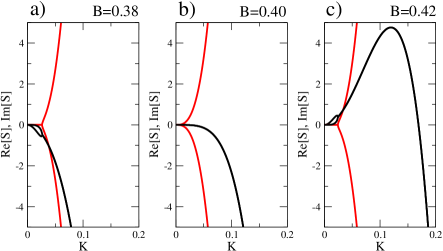
Figure 3: (Color online) Real (solid line) and imaginary (light line) parts of the growth rate $S$ as functions of the wavenumber $K$ of the perturbation for (a) $B=0.38,$ (b) $B=0.4$ and (c) $B=0.42$. Other parameters are $A=0.2$ and $D=0$.

Figure 3 shows dependences $\operatorname{Re}\left[S(K)\right]$ and $\operatorname{Im}\left[S(K)\right]$ at three values of the parameter $B$ below and above the instability boundary. While the fastest growing mode at $B>B_{c\text{ }}$is always oscillatory, with $\operatorname{Im}\left[S(K)\right]\neq 0$, above the instability boundary the system also always has some standing growing modes with the wavenumbers $K$ smaller than $K_{c}$. As the boundary is approached from above, both the wavenumber $K_{c}$ and the frequency $\Omega_{c}$ decrease and vanish at $B=B_{c}$. The region with two real modes $S_{1}(K)$ and $S_{2}(K)$ always lies below $K_{c}$; it shrinks and vanishes at $B=B_{c}$. Similar long-wavelength instabilities have previously been discussed for other conservative systems (see cross1993 ).

IV Numerical Investigations of the Nonlinear Regime

To investigate the behavior of the system in the nonlinear regime above the instability onset, numerical simulations have been performed. Equations(7,8) were integrated using the semi-implicit method (see appendix B) for a one-dimensional system using periodic boundary conditions. As the initial condition, the flat interface with a uniform machine distribution was chosen and small random initial perturbations were applied.

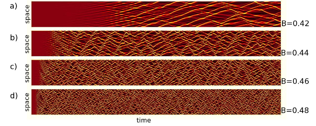
Figure 4: (Color online) Interface turbulence. Space-time diagrams display the local film thickness $H$ (thicker regions correspond to bright and thinner regions to dark colors) depending on the spatial coordinate and time for : (a) $B=0.42$, (b) $B=0.44$, (c) $B=0.46$ and (d) $B=0.48$. Other system parameters are $A=0.2$ and $D=0$. Numerical integrations for a one-dimensional system of length $L_{0}=512$ (with $\Delta x=1$) and the total time interval of $T_{0}=5\cdot 10^{5}$ (with $\Delta t=0.01$).

Our main observation is that the instability development results in the emergence of a complex spatiotemporal regime which can be described as interface turbulence. This regime is characterized by spontaneous appearance of traveling machine clusters (i.e., of spatial regions where the local machine concentration is increased) and of the accompanying local interface modulations.

Figure(4) gives an illustration of the turbulent regimes observed at different different distances from the instability threshold. The local film thickness $H$ is displayed here in gray scale depending on the spatial coordinate (the vertical axis) and time. In the slightly supercritical regime at $B=0.42$, the transient development of standing waves is first observed, which is then followed by the emergence of an irregular pattern of traveling and colliding waves. At larger deviations from the critical point, the transients are faster and the irregular wave dynamics appears soon after the instability onset. The characteristic spatial scale of the turbulence decreases with the control parameter $B$, consistent with the predictions of the linear stability analysis. The characteristic velocity of traveling waves is also growing with $B$.

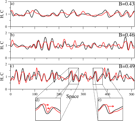
Figure 5: (Color online) Snapshots of the concentration distributions (light lines) and of the respective interface profiles (black lines) for (a) $B=0.43$, (b) $B=0.46$ and (c) $B=0.49.$ Other parameters are $A=0.2$ and $D=0$. Insets on the bottom show the collision of two waves (d) and the motion of a single wave (e). Arrows in the insets indicate the directions of motion of the distribution maxima.

Figure 5 shows snapshots of computed turbulent patterns at different deviations from the instability threshold. Both the interface profiles and the corresponding concentration distributions are presented here. Again, a decrease of the characteristic wavelength of the irregular spatiotemporal patterns under an increase of the control parameter $B$ can be noticed. Moreover, we see that the characteristic amplitude of the waves grows with $B$. To illustrate the directions of wave propagation, arrows are placed in the insets of this figure, where examples of colliding and traveling waves are shown. These arrows indicate the directions in which the respective concentration and interface profile maxima are shifting at the next time moment. Note that the motions of machine clusters (i.e, of the local concentration maxima) are typically guiding the motions of surface bumps.

Temporal transients leading to turbulent patterns are characterized in Fig. 6. To construct it, we have determined the maximum and the minimum values $H_{\max}$ and $H_{\min\text{ }}$of the film thickness as function of time, starting from the initial moment. Their difference $\Delta H(T)=H_{\max}(T)-H_{\min}(T)$ (where $T$ is the dimensionless time) can be chosen to describe the amplitude of the developing patterns. As seen in the two top panels in Fig. 6, this amplitude first grows (exponentially) and the undergoes saturation. The transient is shorter for the larger deviation from the threshold ($B=0.46$) and the final mean amplitude of the turbulent pattern is also then larger.

To estimate the characteristic wavenumber $K_{0}(T)$ of the developing spatial patterns, their Fourier transforms were computed and the positions of dominant maxima in the spatial power spectra were determined at different time moments. As seen in the two bottom panels in Fig. 6, these wavenumbers do not significantly change during the transients. The characteristic wavelengths of the developed turbulent patterns are therefore not much different from those of the critical modes.

Figure 7 shows temporal dependences of the hight $H(T)$ and the concentration $C(T)$ at a fixed point of the system in the final turbulent state. The characteristic time of the oscillations is clearly different for the two values of the control parameter. Both properties fluctuate around some mean values. The fluctuations are more rapid farther away from the instability threshold.

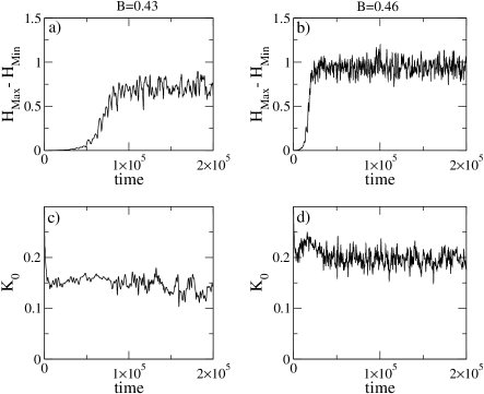
Figure 6: Initial evolution of the pattern amplitudes $\Delta H(T)$ and of the characteristic wavenumbers $K_{0}$ of the developing patterns for two different values $B=0.43$ and $B=0.46$ of the control parameter. Other parameters are $A=0.2$ and $D=0$. The system size is $L_{0}=512.$

Finally, Fig. 8 displays the dependence of several selected statistical properties of the final turbulent state on the deviation $\Delta B=B-B_{c}$ from the critical point $B_{c}$. The characteristic wavenumbers $K_{0}$ and amplitudes $\Delta H$ have been computed as described above. Time averages of these properties and statistical dispersion of the data are shown in Figs. 8. The characteristic transient times $T_{c}$ (Fig. 8c) have been estimated by fitting the initial computed time dependence for $\Delta H(T)$ to the exponential law, $\Delta H(T)\sim\exp(T/T_{c})$. The characteristic frequency $\Omega_{0}$ of the patterns (Fig. 8d) is estimated by computing their temporal power spectra and determining the positions of the dominant maxima.

Solid curves in Fig. 8 give fits of the simulation data to the power laws predicted by the linear stability analysis. According to equations (13) and (14), $K_{c}\sim$ $\Delta B^{1/2}$ and $\Omega_{c}\sim\Delta B^{3/2}$. The transient time is determined by the rate of growth as $T_{c}=1/\operatorname{Re}\left[S_{c}(B)\right]$ and, according to equation (15), we expect that $T_{c}^{-1}\sim\Delta B^{2}$. For the mean amplitude $\Delta H$ of the patterns, the quadratic fit $\Delta H\sim\Delta B^{1/2}$ has been applied. We see that the statistical properties of nonlinear patterns in the developed turbulence regime are still in good agreement with the respective predictions based on the linear stability analysis.

V Discussion and Conclusions

Can predicted interface instabilities be experimentally observed? This question has both chemical and physical aspects. On the chemical side, it is known that proteins may indeed represent surfactants and thus float at the air-water interface (see. e.g., beverung1999 ). Although we cannot give here a specific example, it seems plausible that some protein machines also belong to this class. Moreover, other protein machines, including molecular motors, can probably be made floating by chemical modification, i.e. by attaching to them a hydrophobic group.

The physical question is whether the propulsion forces generated by individual protein machines would be sufficient to induce the considered interface instability. According to equation (12), the instability is reached when $B>B_{c}$ with $B_{c}=2(A+D)$. Taking into account the definitions of dimensionless properties $A$, $B$ and $D$, the instability condition implies that the propulsion force $f,$ generated by a single machine, must exceed the threshold

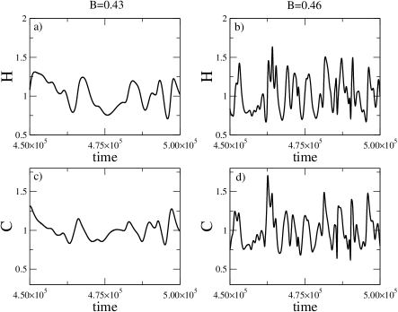
Figure 7: Time dependences of the film hight $H(T)$ and concentration $C(T)$ at a fixed spatial point for two different values of the control parameter $B$. Other parameters and the system length are the same as in Fig.4.

$$f_{c}=\frac{2}{N_{A}}\left(\frac{\sigma_{c}}{h_{0}}+\frac{d\mu}{c_{0}h_{0}^{2}}\right)$$ (16)

where $h_{0}$ is the film thickness, $c_{0}$ is the surface concentration of floating machines, $d$ is their surface diffusion constant, $\mu$ is the liquid viscosity, $N_{A}$ is the Avogadro number, and $\sigma_{c}$ specifies the surfactant capacity of the considered biomolecules (the surface tension coefficient $\sigma$ depends as $\sigma=\sigma_{0}-\sigma_{c}c$ on their concentration $c$).

For numerical order-of-magnitude estimates, we choose $\mu\approx 10^{-2}$ g cm^-1s^-1 (the viscosity of water), $d\approx 10^{-7}$ cm²s^-1 (characteristic diffusion constant of large biomolecules in water solutions kim1992 ). Based on the experimental data given in Ref. beverung1999 , we take furthermore $\sigma_{c}\approx 10^{7}~{}g~{}cm^{2}~{}s^{-2}~{}mMol^{-1}$.

Both terms in equation (16) are inversely proportional to the liquid film thickness $h_{0}$ and the smaller critical forces are therefore expected for the thicker layers. Note, however, that this result is based on the lubrication approximation for thin liquid films, requiring that the film thickness is much smaller than the characteristic wavelength of the flow patterns. As we have seen, the characteristic wavelength of the interface turbulence in the considered system depends on the distance from the critical point (cf. equation (13)) and, in principle, can be arbitrarily large sufficiently close to the instability threshold. Taking into account experimental limitations making it very difficult to work too close to the threshold, we choose however $h_{0}=1mm$ as the characteristic maximum film thickness.

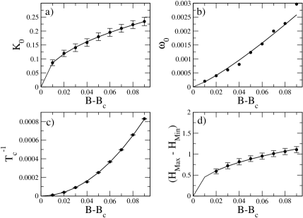
Figure 8: Statistical properties of the interface turbulence at different deviations from the instability threshold: (a) characteristic wavenumber, (b) characteristic frequency, (c) characteristic inverse transient time and (d) mean amplitude of the patterns. Dots show mean values, bars indicate statistical dispersion of numerical data. Solid curves show power laws corresponding to the linear stability analysis predictions (see the text). The same system and simulation parameters as in Fig. 6.

Concentration $c_{0}$ of floating proteins enters only into the second term in equation (16). This term, depending on surface diffusion of floating machines, can be neglected in comparison with the first term, if the condition $c_{0}\gg c_{d}$ with

$$c_{d}=\frac{d\mu}{\sigma_{c}h_{0}}$$ (17)

holds. Substituting numerical values, we get $c_{d}=10^{-18}~{}Mol/cm^{2}$. Thus, already for very low surface concentrations of proteins, effects of their diffusion can be neglected in the considered problem.

Neglecting diffusion effects, the critical propulsion force of a single machine is estimated as

$$f_{c}=\frac{2\sigma_{c}}{N_{A}h_{0}}.$$ (18)

Note that it does not depend on the protein concentration.

Substitution of the numerical values into equation (18) yields $f_{c}=3\cdot 10^{-5}~{}pN$. Can a single molecular machine generate the hydrodynamical propulsion force of that magnitude?

Direct measurements of molecular propulsion forces are still not available. It is known that molecular motors, such as myosin or kinesin, can generate mechanical forces of about $1~{}pN$ Finer1994 ; fisher1999 ; fisher2001 , but these data refers to the molecules moving along microtubules and filaments, not to the swimmers.

For a simple example, we consider the elementary three-body Purcell swimmer purcell1976 . Its characteristic propulsion velocity is about $V=\Delta L/\tau$, where $\Delta L$ is the displacement per single cycle and $\tau$ is the characteristic time of the cycle (cf. becker2003 ; tam2007 ). The viscous friction force of an object of linear size $L$ that moves with velocity $V$ through the liquid is by the order-of-magnitude $f_{0}=6\pi\mu LV$. Thus, propulsion at velocity $V=\Delta L/t_{c}$ would require the propulsion force about $f_{0}=6\pi\mu L\Delta L/t_{c}$. Choosing $L\approx 50$ nm, $\Delta L=0.1L$ and $\tau=1$ ms and considering water as the liquid, we obtain for the molecular propulsion force the rough estimate of $f_{0}=10^{-3}$pN. Similar estimates are obtained for other known elementary swimmers. Note that the actual average propulsion force $f$ of a machine additionally depends on the frequency of machine cycles and the angle with respect the interface, therefore, according to equation (1), this gives the estimate of the maximum propulsion force under the energy-supply saturation conditions and the most efficient orientation of the machine.

While molecular propulsion forces are quite small, according the above estimates they would still be sufficient to induce the film instability and lead to the interface turbulence. Therefore, we conclude that the experimental observation of the predicted effects is principally possible.

The experiments aimed at detecting instabilities of thin liquid layers induced by floating actively operating machines would allow to directly estimate actual propulsion forces generated by particular biomolecules. Investigations of such nonequilibrium hydrodynamical systems would be very important from the perspective of active microfluidics, where active motions in thin liquid layers are produced by floating biomolecular propellers.

Financial support from the EU Marie Curie RTN ”Unifying principles in nonequilibrium pattern formation” and from the German Science Foundation Collaborative Research Center SFB 555 ”Complex Nonlinear Processes” is acknowledged. We are grateful to U. Steiner, D. Barbero and U. Thiele for valuable discussions.

Appendix A Hydrodynamic equations

We consider the situation when the film thickness $h_{0}$ is the smallest characteristic length of the system. In this case, the lubrication approximation can be used which corresponds to an expansion in the small parameter $\epsilon=h_{0}/\lambda$, with $\lambda$ being the characteristic wavelength of the patterns in the lateral direction. Hydrodynamical equations in the lubrication approximation are simplified and take the form (see, e.g., oron1997 )

$$\mu\partial_{zz}\vec{u}=\vec{\nabla}p,$$

$$\partial_{z}p=0,$$ (19)

with the incompressibility condition

$$\vec{\nabla}\vec{u}+\partial_{z}w=0.$$ (20)

Here, $w$ is the vertical component of the fluid velocity and $\vec{u}$ is its horizontal component; $\vec{\nabla}$ is the differential operator acting only on the horizontal coordinates. Note that, as follows from these equations, pressure $p$ is constant along the vertical direction.

The boundary conditions at the bottom of the film, in contact with the solid support, are

$$w=\vec{u}=0\text{ at }z=0.$$

At the free air-liquid interface $z=h$, the balance of horizontal and vertical forces should separately hold, implying that

$$\mu\partial_{z}\vec{u}=\vec{\nabla}\sigma,$$ (21)

$$p=-\sigma\nabla^{2}h-p_{m},$$ (22)

where $\sigma$ is the surface tension coefficient and $p_{m}$ is the additional pressure produced by floating active molecules.

Conservation of the total film volume implies moreover that the equation.

$$\partial_{t}h+\vec{\nabla}\left(\int_{0}^{h}\vec{u}dz\right)=0$$ (23)

should hold.

Integrating equations.(19) and taking into account the boundary condition (22), the horizontal velocity of the flow can be determined,

$$\vec{u}=\frac{1}{\mu}\left[\vec{\nabla}p\left(\frac{z^{2}}{2}-hz\right)+z\vec{\nabla}\sigma\right].$$ (24)

The vertical velocity is then obtained by using the incompressibility condition,

$$w=-\frac{1}{2\mu}\left(\nabla^{2}p\left(\frac{z^{3}}{3}-z^{2}h\right)-z^{2}\vec{\nabla}p\vec{\nabla}h+z^{2}\nabla^{2}\sigma\right)$$ (25)

Substituting these expressions into equation (23) and integrating over $z$, the final form of the interface equation is derived,

$$\partial_{t}h=\frac{1}{\mu}\vec{\nabla}\left(\frac{h^{3}}{3}\vec{\nabla}p-\frac{h^{2}}{2}\vec{\nabla}\sigma\right).$$ (26)

Appendix B Numerical Integration Method

While simple explicit Euler methods are frequently employed in numerical investigations of nonlinear reaction-diffusion models, such methods easily become numerically unstable when hydrodynamical microfluidics equations are considered. Therefore, a specially constructed numerical integration method has been employed in our study. Below, its brief description is provided.

There are two nonlinear differential equations to solve, one for the thickness $H$ and the other for the concentration $C$ of the surfactant. We define vector $\vec{U}=(H,C)$ and formally write both equations as

$$\partial_{t}\vec{U}=\mathbf{F}(\vec{U})$$ (27)

The matrix operator $\mathbf{F}$ can be decomposed as $\mathbf{F=L}\vec{U}+\mathbf{N}(\vec{U})$ into its linear ($\mathbf{L}\vec{U}$) and nonlinear ($\mathbf{N}(\vec{U})$) parts. They are defined as

$$\mathbf{L=}\left.\frac{\delta\mathbf{F}(\vec{U})}{\delta\vec{U}}\right|_{\vec{U}=\vec{U}_{0}},\text{ \ }\mathbf{N}(\vec{U})=\text{\ }\mathbf{F}(\vec{U})-\mathbf{L}\vec{U}.$$ (28)

To compute $\vec{U}(t+\Delta t)$ at the next time step $t+\Delta t$, the mixed semi-implicit method is employed:

$$\vec{U}(t+\Delta t))-\Delta t\mathbf{L}\vec{U}(t+\Delta t)=\vec{U}(t)+\Delta t\mathbf{N}(\vec{U}(t)).$$ (29)

Thus, the implicit method is used to determine the contribution from the linear part in time $t+\Delta t$ and the explicit method is employed to compute the nonlinear part contribution.

Applying the inverse matrix operator $(1-\Delta t\mathbf{L})^{-1}$ to both sides of this equation yields

$$\vec{U}(t+\Delta t)=(1-\Delta t\mathbf{L})^{-1}\left(\vec{U}(t)+\Delta t\mathbf{N}(\vec{U}(t))\right)$$

Recombining some terms and using $\mathbf{F=L}\vec{U}+\mathbf{N}(\vec{U})$, the final finite-difference equation is obtained

$$\vec{U}(t+\Delta t)=\vec{U}(t)+\Delta t(1-\Delta t\mathbf{L})^{-1}\mathbf{F}(\vec{U}(t))$$

The calculation of the inverse differential matrix operator $(1-\Delta t\mathbf{L})^{-1}$ is most conveniently performed by transforming the equation to the Fourier space. Here, it is important that the term $\mathbf{F}(\vec{U}(t))$ is determined before applying the Fourier transformation.

Our simulations using this numerical method have been performed only in the one-dimensional case, $H=H(x,t)$ and $C=C(x,t)$. In two dimensions, the method becomes complicated and such simulations have not been undertaken.

References

- (1) E. R. Kay, D. A. Leigh and F. Zerbetto, Angew. Chem. Int. Ed. 46, 72 (2007).
- (2) Y. Togashi and A. S. Mikhailov, Proc. Natl. Acad. Sci. USA 104, 8697 (2007)
- (3) E. M. Purcell, Amer. J. Phys. 45, 3 (1977).
- (4) A. Shapere and F. Wilczek, Phys. Rev. Lett. 58, 2051 (1987).
- (5) L. E. Becker, S. A. Koehler and H. A. Stone, J. Fluid Mech. 490, 15 (2003).
- (6) A. Najafi and R. Golestanian, Phys. Rev. E 69, 062901 (2004).
- (7) D. J. Earl, C. M. Pooley, J. F. Ryder, I. Bredberg and J. M. Yeomans, J. Chem. Phys. 126, 064703 (2007)
- (8) R. Golestanian and A. Ajdari, Phys. Rev. E 77, 036308 (2008).
- (9) R. Golestanian and A. Ajdari, Phys. Rev. Lett. 100, 038101 (2008).
- (10) S. Ramaswamy, J. Toner and J. Prost, Phys. Rev. Lett. 84, 3494 (2000).
- (11) V. Casagrande, Y. Togashi, A. S. Mikhailov, Phys. Rev. Lett. 99, 048301 (2007).
- (12) C. J. Beverung, C. J. Radke and H. W. Blanch, Biophys. Chem. 81, 59 (1999).
- (13) A. Oron, S. H. Davis and S. G. Bankoff, Rev. Mod. Phys. 69, 931 (1997).
- (14) A. De Wit, D. Gallez and C. I. Christov, Phys. Fluids 6, 3256 (1994).
- (15) M. C. Cross and P. C. Hohenberg, Rev. Mod. Phys. 65, 851 (1993).
- (16) S. Kim and H. Hu, J. Phys. Chem 96, 4034 (1992).
- (17) J. T. Finer, R. M. Simmons and J. A. Spudich, Nature 368, 113 (1994).
- (18) M. E. Fisher and A. B. Kolomeisky, Proc. Natl. Acad. Sci. USA 96, 6597 (1999).
- (19) M. E. Fisher and A. B. Kolomeisky, Proc. Natl. Acad. Sci. USA 98, 7748 (2001).
- (20) D. Tam and A. E. Hosoi, Phys. Rev. Lett. 98, 068105 (2007).