A simple reaction-diffusion population model on scale-free networks

Abstract

We study a simple reaction-diffusion population model (proposed by A. Windus and H. J. Jensen, J. Phys. A: Math. Theor. 40, 2287 (2007)) on scale-free networks. In the case of fully random diffusion, the network topology does not affect the critical death rate, whereas the heterogenous connectivity makes the steady population density and the critical population density small. In the case of modified diffusion, the critical death rate and the steady population density are higher, at the meanwhile, the critical population density is lower, which is good for survival of species. The results are obtained with a mean-field framework and confirmed by computer simulations.

Recently, Windus and Jensen jpa07 ; tpb07 introduced a model for population on lattices with diffusion and birth/death according to $2A\rightarrow 3A$ and $A\rightarrow\phi$ for an individual $A$ . They found that the model displays a phase transition from an active to an absorbing state which is continuous in $1+1$ dimensions and of first-order in higher dimensions jpa07 . They also investigated the importance of fluctuations and that of the population density, particularly with respect to Allee effects in regular lattices tpb07 . It was found that there exists a critical population density below which the probability of extinction is greatly increased, and the probability of survival for small populations can be increased by a reduction in the size of the habitat tpb07 .

In the study of complex networks Albert , an important issue is to investigate the effect of their complex topological features on dynamical processes review07 , such as the spread of infectious diseases pv01a and the reaction-diffusion (RD) process GA04 . For most real networks, the connectivity distribution has power-law tails $P(k)\sim k^{-\gamma}$, namely, a characteristic value for the degrees is absent, hence the scale-free (SF) property. In this Brief Report, we shall study the simple RD population model jpa07 on SF networks.

In an arbitrary finite network which consists of nodes $i=1,\ldots,N$ and links connecting them. Each node is either occupied by a single individual (1) or empty (0). We randomly choose a node. If it is occupied, the individual dies with probability $p_{\rm d}$, leaving the node empty. If the individual does not die, a nearest neighbor-node is randomly chosen. If the neighboring node is empty, the particle moves there; otherwise, the individual reproduces with probability $p_{\rm b}$ producing a new individual on another randomly selected neighboring node, conditional on that node being empty. A time step is defined as the number of network nodes $N$. In homogeneous networks (such as regular lattices and Erdös-Rényi (ER) random networks erdos59 ), the mean-field (MF) equation for the density of active nodes $\rho(t)$ is given by tpb07

$$\frac{d\rho(t)}{dt}=-p_{\rm d}\rho(t)+p_{\rm b}(1-p_{\rm d})\rho^{2}(t)(1-\rho(t)),$$ (1)

which has three stationary states

$$\bar{\rho}_{0}=0,\quad\bar{\rho}_{\pm}=\frac{1}{2}\left(1\pm\sqrt{1-\frac{4p_{\rm d}}{p_{\rm b}(1-p_{\rm d})}}\right).$$ (2)

For $4p_{\rm d}>p_{\rm b}(1-p_{\rm d})$, $\bar{\rho}_{0}$ is the only real stationary state, and one can obtain a critical death rate $p_{{\rm d}_{\rm c}}=p_{\rm b}/(4+p_{\rm b})$ which separates the active phase representing survival and the absorbing state of extinction. Simple analysis shows that $\bar{\rho}_{+}$ and $\bar{\rho}_{0}$ are stable stationary states, whereas $\bar{\rho}_{-}$ is unstable and therefore represents a critical density $\rho_{\rm c}$ below which extinction will occur in all cases. Thus, for $p_{\rm d}<p_{{\rm d}_{\rm c}}$, one can write tpb07

$$\rho(t)\rightarrow\left\{\begin{array}[]{cl}0&\text{if}\quad\rho(t)<\rho_{\rm c},\\ \bar{\rho}_{+}&\text{if}\quad\rho(t)>\rho_{\rm c},\end{array}\right.\quad\text{as}\quad t\rightarrow\infty.$$ (3)

At $p_{\rm d}=p_{{\rm d}_{\rm c}}$, the stationary density jumps from $1/2$ to $0$, resulting in a first-order phase transition.

In order to study analytically this process on SF networks in which the degree distribution has the form $P(k)\sim k^{-\gamma}$ and nodes show large degree fluctuations, we are forced to consider the partial densities $\rho_{k}(t)$, representing the density of individuals in nodes of degree $k$ at time $t$ pv01a . To obtain a rate equation for $\rho_{k}(t)$ , we use a microscopical approach which has been applied in diffusion-annihilation da05 and multicomponent RD processes on SF networks mrd06 . Let $n_{i}(t)$ be a dichotomous random variable taking values $0$ or $1$ whenever node $i$ is empty or occupied by an individual $A$, respectively. Using this formulation, the state of the system at time $t$ is completely defined by the state vector ${\bf n}(t)=\{n_{1}(t),n_{2}(t),\cdots,n_{N}(t)\}$. The evolution of ${\bf n}(t)$ after a time step can be expressed as

$$n_{i}(t+1)=n_{i}(t)\eta+[1-n_{i}(t)]\xi,$$ (4)

where $\eta$ and $\xi$ are dichotomous random variables, taking values of $0$ or $1$ with certain probabilities $p$ and $1-p$, respectively,

$$\eta=\left\{\begin{array}[]{cl}0;&\displaystyle{p=p_{\rm d}+(1-p_{\rm d})\left[1-\frac{1}{k_{i}}\sum_{j}a_{ij}n_{j}(t)\right]},\\[14.22636pt] 1;&\displaystyle{1-p},\end{array}\right.$$ (5)

$$\xi=\left\{\begin{array}[]{cl}1;&\displaystyle p=\displaystyle{\sum_{j}\frac{(1-p_{\rm d})a_{ij}n_{j}(t)}{k_{j}}\left[1+\frac{p_{\rm b}}{k_{j}}\sum_{l}a_{jl}n_{l}(t)\right]},\\[14.22636pt] 0;&\displaystyle{1-p}\end{array}\right.$$ (6)

Obviously, $p$ is the probability that an occupied node $i$ becomes empty. If node $i$ is empty, there are two factors causing it occupied. One is that its survival neighbors will move to $i$ with probability $\sum_{j}\frac{(1-p_{\rm d})a_{ij}n_{j}(t)}{k_{j}}$ and the other is that its survival neighbor $j$ selecting an occupied neighbor $l$ (with the probability $\frac{1}{k_{j}}\sum_{l}a_{jl}n_{l}(t))$) reproduces a new individual on $i$, then we have the term $\sum_{j}\frac{(1-p_{\rm d})a_{ij}n_{j}(t)}{k_{j}}\frac{p_{\rm b}}{k_{j}}\sum_{l}a_{jl}n_{l}(t))$. Taking the average of Eq. (4), we obtain

$$\langle n_{i}(t+1)|{\bf n}(t)\rangle = n_{i}(t)(1-p_{\rm d})\frac{1}{k_{i}}\sum_{j}a_{ij}n_{j}(t)+(1-n_{i}(t))\left[\sum_{j}\frac{(1-p_{\rm d})a_{ij}n_{j}(t)}{k_{j}}(1+\frac{p_{\rm b}}{k_{j}}\sum_{l}a_{jl}n_{l}(t))\right],$$ (7)

which describes the average evolution of the system, conditioned to the knowledge of its state at the previous time step. In the MF approximation, $\langle n_{i}(t)n_{j}(t)\rangle\equiv\langle n_{i}(t)\rangle\langle n_{j}(t)\rangle$ and $\langle n_{i}(t)n_{j}(t)n_{l}(t)\rangle\equiv\langle n_{i}(t)\rangle\langle n_{j}(t)\rangle\langle n_{l}(t)\rangle$. Thus, after multiplying Eq. (7) by the probability to find the system at state ${\bf n}$ at time $t$ and summing for all possible configurations, we obtain

$$\rho_{i}(t+1) \equiv \langle n_{i}(t+1)\rangle=\rho_{i}(t)\frac{(1-p_{\rm d})}{k_{i}}\sum_{j}a_{ij}\rho_{j}(t)+(1-\rho_{i}(t))\left[\sum_{j}\frac{(1-p_{\rm d})a_{ij}\rho_{j}(t)}{k_{j}}(1+\frac{p_{\rm b}}{k_{j}}\sum_{l}a_{jl}\rho_{l}(t))\right].$$ (8)

We assume that nodes with the same degree are statistically equivalent, i.e.,

$$\rho_{i}(t)\equiv\rho_{k}(t)\quad\forall i\in\mathcal{V}(k),$$ (9)

and have

$$\sum_{j}a_{ij}=\sum_{k^{\prime}}\sum_{j\in\mathcal{V}(k^{\prime})}a_{ij}=\sum_{k^{\prime}}kP(k^{\prime}|k)\quad\forall i\in\mathcal{V}(k),$$ (10)

where $\mathcal{V}(k)$ is the set of nodes of degree $k$.

We split the sum with index $j$ into two sums over $k^{\prime}$ and $\mathcal{V}(k^{\prime})$, respectively. The double sum over $a_{ij}$ is related to the conditional probability $P(k^{\prime}|k)$ that a node of given degree $k$ has a neighbor which has degree $k^{\prime}$. In present work, we restrict ourselves to the case of uncorrelated networks in the following, in which the conditional probability takes the simple form $P(k^{\prime}|k)=k^{\prime}P(k^{\prime})/\langle k\rangle$. Thus, from Eq. (8) and after some formal manipulations, we obtain

$$\rho_{k}(t+1)=\rho_{k}(t)(1-p_{\rm d})\Theta(\rho(t))+\frac{k}{\langle k\rangle}(1-p_{\rm d})(1-\rho_{k}(t))\rho(t)[1+p_{\rm b}\Theta(\rho(t))],$$ (11)

where $\rho(t)$ is the total density of active individuals and $\Theta(\rho(t))$ is the probability that any given link points to an occupied node

$$\Theta(\rho(t))=\frac{1}{\langle k\rangle}\sum_{k}kP(k)\rho_{k}(t).$$ (12)

From Eq. (11), we can obtain the following rate equation

$$\frac{d\rho_{k}(t)}{dt}=-\rho_{k}(t)+\rho_{k}(t)(1-p_{\rm d})\Theta(t)+\frac{k}{\langle k\rangle}(1-p_{\rm d})(1-\rho_{k}(t))\rho(t)[1+p_{\rm b}\Theta(\rho(t))].$$ (13)

Imposing stationarity $\partial_{t}\rho_{k}(t)=0$, we obtain

$$\rho_{k}=\frac{\frac{k}{\langle k\rangle}(1-p_{\rm d})\rho(1+p_{\rm b}\Theta(\rho))}{\cosh+\frac{k}{\langle k\rangle}(1-p_{\rm d})\rho(1+p_{\rm b}\Theta(\rho))}.$$ (14)

This set of equations imply that the higher the node connectivity, the higher the probability to be in an occupied state. This inhomogeneity must be taken into account in the computation of $\Theta(\rho)$. Multiplied Eq. (13) by $P(k)$ and summing over $k$, we obtain a rate equation for $\rho(t)$

$$\frac{d\rho(t)}{dt}=-\rho(t)p_{\rm d}+p_{\rm b}(1-p_{\rm d})[1-\Theta(\rho(t))]\rho(t)\Theta(\rho(t)),$$ (15)

Notable, the above equation is consistent with Eq. (1) by imposing that $\Theta(\rho(t))=\rho(t)$ in homogeneous networks. It also has three stationary states

$$\bar{\rho}^{SF}_{0}=0,\quad\Theta(\bar{\rho}^{SF}_{\pm})=\bar{\rho}_{\pm}=\frac{1}{2}\left(1\pm\sqrt{1-\frac{4p_{\rm d}}{p_{\rm b}(1-p_{\rm d})}}\right).$$ (16)

The critical death rate $p_{{\rm d}_{\rm c}}=p_{\rm b}/(4+p_{\rm b})$ is the same as that in homogeneous networks. Imposing, naturally, $\frac{d\Theta(\rho)}{d\rho}>0$, we find that $\bar{\rho}^{SF}_{+}$ and $\bar{\rho}^{SF}_{0}$ are stable stationary states, whereas $\bar{\rho}^{SF}_{-}$ is unstable and therefore represents a critical density $\rho^{SF}_{\rm c}$ below which extinction will occur in all cases. In SF networks, the higher the node connectivity, the higher the probability to be in an occupied state (Eq. (14)). The presence of nodes with very large degree results in that $\bar{\rho}^{SF}_{\pm}<\Theta(\bar{\rho}^{SF}_{\pm})$. We conclude that both the population steady state and the critical population in SF networks are smaller than those in homogeneous networks.

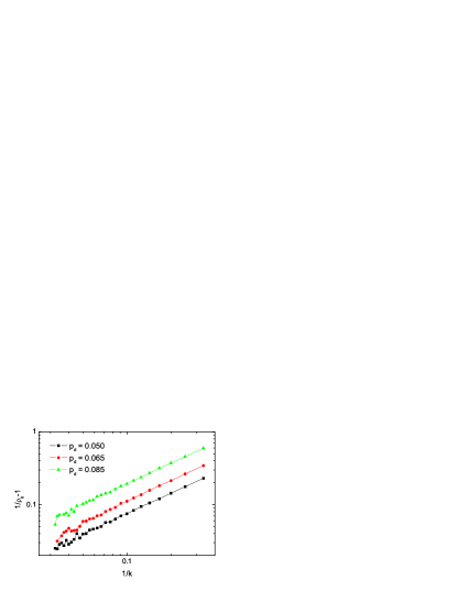
Figure 1: Simulation results of $\frac{1}{\rho_{k}}-1$ against the reciprocal of $k$ in log-log scale on uncorrelated random SF networks with exponent $\gamma=3.0$, $k_{min}=3$ and $N=10^{3}$. The birth rate is $p_{\rm b}=0.5$. All the plots recover the form predicted in Eq. (14).

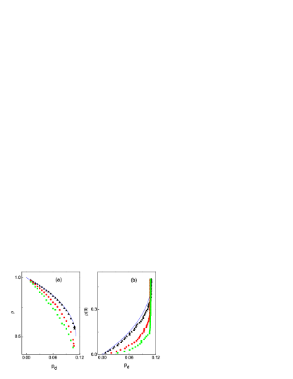
Figure 2: (a) Stationary population densities $\rho$ against the death rate $p_{\rm d}$. (b) For different death rate $p_{\rm d}$, there are different critical initial population densities $\rho(0)$. All the data were obtained with $p_{\rm b}=0.5$ and $N=1000$. MF results for the homogenous network (line) and simulation results for the ER random network (triangles), uncorrelated random SF networks with exponent $\gamma=3.0$ (circles) and $2.5$ (squares).

The numerical simulations performed on uncorrelated SF networks confirm the picture extracted from the analytic treatment. We construct the uncorrelated SF network by the algorithm ucmmodel with minimum degree $k_{\text{{min}}}=3$ and size $N=1000$. The simulations are carried out on an initially fully occupied network for obtaining $\rho_{k}$ and steady states. To find the critical population density, due to its instability, we instead use the initial population density $\rho(0)$ and find the value of $p_{\rm d}$ that separates the active and absorbing states. The prevalence $\rho_{k}$ is computed and averaged over $100$ times for each network configuration, which are performed on $10$ different realizations of the network. Figure 1 shows the behavior of the probability $\rho_{k}$ that a node with degree $k$ is occupied. The numerical value of the slope in log-log scale is about $0.98$, which is in good agreement with the theoretical value $1$ in Eq. (14). In Fig. 2, for ER networks with average degree $\langle k\rangle=14$ and size $N=1000$, both plots of the stationary population density $\rho$ and the critical initial population density $\rho(0)$ are consistent with the MF results in homogenous networks (Eq. (2)). For SF networks, the population and the critical initial population density in steady states are smaller than that of homogeneous networks, which agrees with Eq. (16). Furthermore, the more heterogeneous the SF network, i.e., the smaller degree exponent of the SF network, the smaller the densities. Noting that in despite of the different network topologies, the critical death rate $p_{{\rm d}_{\rm c}}$ is changeless, which is the prediction of Eq. (16).

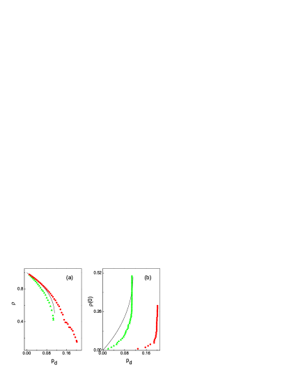
Figure 3: (a) Stationary population densities $\rho$ against the death rate $p_{\rm d}$. (b) Critical initial population densities $\rho(0)$ versus the death rate $p_{\rm d}$. All the data were obtained with $p_{\rm b}=0.5$ and $N=1000$. MF results for the homogenous network (line), simulation results in the uncorrelated random SF networks with exponent $\gamma=3.0$ with fully random diffusion (triangles), and the modified diffusion under $\alpha=1$ and $\beta=-2$ (circles).

In the above model, the neighboring node is chosen with full randomness, and we call this fully random diffusion. In the following, we shall redesign the diffusion strategies of the population model on SF networks. If the randomly chosen particle does not die, a nearest neighbor node $j$ is randomly chosen with a probability proportional to $k^{\alpha}_{j}$. If the neighboring node $j$ is empty, the particle moves there; otherwise, the particle reproduces with probability $p_{\rm b}$ producing a new particle on another neighboring node $l$ which is chosen by a probability proportional to $k^{\beta}_{l}$, conditional on that node being empty. We can also write the MF equation in the uncorrelated random SF network for this modified diffusion case

$$\frac{d\rho(t)}{dt}=-\rho(t)p_{\rm d}+p_{\rm b}(1-p_{\rm d})(1-\Theta_{\beta}(\rho(t)))\rho(t)\Theta_{\alpha}(\rho(t)),$$ (17)

where

$$\Theta_{\alpha}(\rho(t))=\frac{1}{\langle k^{1+\alpha}\rangle}\sum_{k}k^{1+\alpha}P(k)\rho_{k}(t).$$ (18)

In the extinction state $\rho(t)=0$, it is natural that $\Theta_{\alpha}(\rho(t))=0$. We can obtain at lowest order in $\rho(t)$, $\Theta_{\alpha}(\rho(t))\simeq A\rho(t)$. Similarly $\Theta_{\beta}(\rho(t))\simeq B\rho(t)$ can also be obtained at lowest order in $\rho(t)$, where $A$ and $B$ are coefficients. In the steady state, following previous analysis, we can easily get the critical death rate

$$p_{{\rm d}_{\rm c}}=\frac{p_{\rm b}}{(4\frac{B}{A}+p_{\rm b})},$$ (19)

which can be changed by the ratio $B/A$. If $B<A$, the modified model has larger critical death rates than the original. Similar to Eq. (14), the partial density takes the form $(\frac{1}{\rho_{k}}-1)\sim 1/D(k)$ with $D(k)=\frac{k^{1+\alpha}}{\langle k^{1+\alpha}\rangle}+\frac{k^{1+\beta}}{\langle k^{1+\beta}\rangle}p_{\rm b}\Theta_{\alpha}$. Considering that $0<p_{\rm b}$ and $\Theta_{\alpha}<1$, we can negate the second term in $D(k)$. If $\alpha>-1$, the higher degree node has larger partial density $\rho_{k}$. As $\beta<\alpha$, we get $B<A$; On the other hand, if $\alpha<-1$, the higher degree node has smaller $\rho_{k}$. As $\beta>\alpha$, we have $B<A$.

In Fig. 3 the diffusion coefficients are $\alpha=1$ and $\beta=-2$. From the previous discussion, we obtain $B<A$. Thus, the modified model has a larger critical death rate. Furthermore, it has the larger steady population density and the smaller critical population density. From the view of conservation, it is better that a population system has a larger critical death rate, a larger steady population density and a lower critical population density at the same time. Our modified model has this nice property under the condition of $B<A$.

In summary, we have studied a simple RD population model on SF networks by analytical methods and computer simulations. We find that in the case of fully random diffusion, the network topology can not change the value of the critical death rate $p_{{\rm d}_{\rm c}}$. However, the more heterogenous the network, the smaller steady population density and the critical population density. For the modified diffusion strategy, we can obtain the larger critical death rate and the higher steady population density, at the meanwhile, the lower critical population density, which is good for the specie’s survival. In present work, we consider the population model which has only one specie, it may be more interesting to investigate population models having multi-species with predator-prey, mutualistic, or competitive interactions in complex networks, which is left to future work.

This work was partially supported by NSFC/10775060, SOCIALNETS, and POCTI/FIS/61665.

References

- (1) A. Windus and H. J. Jensen, J. Phys. A: Math. Theor. 40, 2287 (2007).
- (2) A. Windus and H. J. Jensen, Theor. Popul. Biol. 72, 459 (2007).
- (3) R. Albert and A.-L. Barabási, Rev. Mod. Phys. 74, 47 (2002); S. N. Dorogovtsev and J. F. F. Mendes, Adv. Phys. 51, 1079 (2002); M. E. J. Newman, SIAM Rev. 45, 167 (2003).
- (4) S. N. Dorogovtsev, A. V. Goltsev and J. F. F. Mendes, arXiv:0705.0010
- (5) R. Pastor-Satorras and A. Vespignani, Phys. Rev. Lett. 86, 3200 (2001).
- (6) L. K. Gallos and P. Argyrakis, Phys. Rev. Lett. 92, 138301 (2004).
- (7) P. Erdös and A. Rényi, Publ. Math. 6, 290 (1959).
- (8) M. Catanzaro, M. Boguñá and R. Pastor-Satorras, Phys. Rev. E 71, 056104 (2005).
- (9) S. Weber and M. Porto, Phys. Rev. E 74, 046108 (2006).
- (10) M. Catanzaro, M. Boguñá and R. Pastor-Satorras, Phys. Rev. E 71, 027103 (2005).