Lévy Flights of Binary Orbits due to Impulsive Encounters

Abstract

We examine the evolution of an almost circular Keplerian orbit interacting with unbound perturbers. We calculate the change in eccentricity and angular momentum that results from a single encounter, assuming the timescale for the interaction is shorter than the orbital period. The orbital perturbations are incorporated into a Boltzmann equation that allows for eccentricity dissipation. We present an analytic solution to the Boltzmann equation that describes the distribution of orbital eccentricity and relative inclination as a function of time. The eccentricity and inclination of the binary do not evolve according to a normal random walk but perform a Lévy flight. The slope of the mass spectrum of perturbers dictates whether close gravitational scatterings are more important than distant tidal ones. When close scatterings are important, the mass spectrum sets the slope of the eccentricity and inclination distribution functions. We use this general framework to understand the eccentricities of several Kuiper belt systems: Pluto, $2003~{}{\rm EL_{61}}$, and Eris. We use the model of Tholen et al. (2007) to separate the non-Keplerian components of the orbits of Pluto’s outer moons Nix and Hydra from the motion excited by interactions with other Kuiper belt objects. Our distribution is consistent with the observations of Nix, Hydra, and the satellites of $2003~{}{\rm EL_{61}}$and Eris. We address applications of this work to objects outside of the solar system, such as extrasolar planets around their stars and millisecond pulsars.

1. Introduction

Several binary Kuiper belt objects (KBOs) have well-measured small orbital eccentricities (Noll et al., 2007). Stern et al. (2003) investigate numerically the forcing of the eccentricity of the Pluto-Charon orbit by interloping KBOs. They find that the system almost never possesses an eccentricity as high as the observed value of 0.003 (Tholen et al., 2007); depending on the model of tidal damping used, they find median values of $10^{-5}-10^{-4}$. Our goal is to develop an analytic theory that describes the effects of a population of unbound perturbers on a binary orbit and can be applied simply to any binary, in the Kuiper belt or elsewhere.

The interaction of a binary system with its environment has been studied extensively in the literature (Heggie, 1975; Sigurdsson & Phinney, 1995; Yu, 2002; Matsubayashi et al., 2007; Sesana et al., 2007). One interesting context is white dwarf-pulsar binaries, which are expected to be circular. For these objects pulse timing produces very accurate measurements of their orbital motion; such measurements reveal that their eccentricities are typically very small but finite, around $10^{-4}-10^{-5}$ (Stairs, 2004). Phinney (1992) investigated the effects of passing stars on the orbit of such a binary and found that for Galactic pulsars, the perturbations are sub-dominant compared to the effects of atmospheric fluctuations in the companion star. The higher density environment of a globular cluster however can induce an order of magnitude higher eccentricity. Rasio & Heggie (1995) and Heggie & Rasio (1996) present a detailed account of the changes in orbital parameters for binaries in a stellar cluster. The work of these authors focuses on the regime where a perturbing body interacts with the binary on timescales longer than the orbital period of the binary. In the Kuiper belt, a single interaction between a binary and an unbound object occurs over a shorter timescale than the orbital period of the binary. We focus on this regime, where the perturbations to the orbital dynamics can be approximated as discrete impulses.

The main result of this work is that we have identified the perturbative evolution of the eccentricity and relative inclination of a nearly circular binary orbit as a Lévy flight, a specific type of random walk through phase space (Shlesinger et al., 1995). The entire distribution function of the eccentricity and inclination is then determined by calculating the frequency of perturbations as a function of their magnitude. We find a simple analytic expression for this distribution function.

We take the following steps to arrive at our conclusion. In section 2 we calculate the effect of one perturber on a two-body orbit, examining separately the tidal effects of distant scatterings, close encounters with a single binary member, and direct collisions. We describe the effects of many such encounters in section 3, and write a Boltzmann equation that describes the distribution function of the orbital eccentricity and the inclination of the binary relative to its initial plane. The quantitative description of the binary’s evolution given by this distribution function reveals its nature as a Lévy flight. In section 4, we allow for a distribution of perturbing masses and discuss the different Lévy distributions that result.

We then use the analytic theory to examine the orbits of binary KBOs being perturbed by the other members of the Kuiper belt. Section 5 applies our analysis to several specific Kuiper belt binaries. We briefly discuss the relevance of this theory to other astrophysical systems in section 6, and summarize our conclusions in section 7.

2. A Single Encounter

We use the following terminology to describe the geometry of the encounter between a single perturber and a two-body orbit. We refer to the two bound bodies as “the binary.” The members of the binary have masses $m_{1}$ and $m_{2}$, with a total mass labeled $m_{b}=m_{1}+m_{2}$ and $m_{1}\geq m_{2}$. The position of body 2 relative to body 1 is given by $\mathbf{r}_{b}$, and the relative velocity by $\mathbf{v}_{b}$. We distinguish between the magnitude and direction of a vector with the notation $\mathbf{r}_{b}=r_{b}\hat{r}_{b}$. We assume $v_{b}\approx\Omega r_{b}$, where $\Omega$ is the orbital frequency of the binary. We write the orbital period as $T_{\rm orb}=2\pi/\Omega$.

We label the mass of the perturber $m_{p}$. The position of the perturber as a function of time, $\mathbf{r}_{p}(t)$, is described by two vectors: $\mathbf{r}_{p}(t)=\mathbf{b}+\mathbf{v}_{p}t$. The vector $\mathbf{b}$ specifies the closest point of the perturber’s trajectory to body 1, and $\mathbf{v}_{p}$ is velocity of the perturber relative to body 1. Each encounter geometry is uniquely specified by $\mathbf{b}$ and $\mathbf{v}_{p}$ under the constraint $\mathbf{b}\cdot\mathbf{v}_{p}=0$. Figure 1 depicts the arrangement of the vectors $\mathbf{r}_{b},\mathbf{v}_{b},\mathbf{r}_{p}(t),\mathbf{b},$ and $\mathbf{v}_{p}$. We assume $T_{\rm orb}\gg b/v_{p}$ so that we may ignore the motion of the binary during the interaction. We further assume that the effects of the gravity of the binary on the perturber are small; the perturber then travels along a straight path with a constant $\mathbf{v}_{p}$. This assumption requires the criterion of $v_{p}^{2}\gg G(m_{b}+m_{p})/b$. If $b$ is small, the perturber may collide with a member of the binary. In this case the assumption that the path of the perturber is unaffected by the gravity of the binary is true under the condition that $v_{p}$ is much greater than the escape velocity of that member of the binary. The escape velocity from body 1 is defined $v^{2}_{{\rm esc,1}}=2Gm_{1}/R_{1}$, where $R_{1}$ is the radius of body 1.

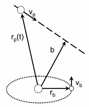
Figure 1.— An illustration of the notation we use to denote the geometry of each perturbation. The dotted line is the almost circular orbit of the binary viewed at an angle. The dashed line is the path of the perturber, given by $\mathbf{r}_{p}(t)=\mathbf{b}+\mathbf{v}_{p}t$.

We are assuming that the timescale of the interaction is much shorter than the orbital timescale, such that the perturbation instantaneously changes the velocities of the binary objects. The impulse provided to a specific member of the binary is found by integrating the acceleration caused by the perturber over its path:

$$\Delta\mathbf{v}_{j}=\int_{-\infty}^{\infty}\frac{Gm_{p}(\mathbf{b}_{j}+\mathbf{v}_{p}t)}{|\mathbf{b}_{j}+\mathbf{v}_{p}t|^{3}}dt=2\frac{Gm_{p}}{v_{p}}\frac{\hat{b}_{j}}{b_{j}},$$ (1)

where the index $j$ specifies whether the impulse $\Delta\mathbf{v}_{j}$ and impact parameter $\mathbf{b}_{j}$ are with respect to either the primary ($j=1$) or the secondary ($j=2$). For the primary, $\mathbf{b}_{1}=\mathbf{b}$ as we have defined it above. For encounters with the secondary, $\mathbf{b}_{2}$ is related to $\mathbf{b}$ by enforcing that it is also perpendicular to $\mathbf{v}_{p}$. Thus we find $\mathbf{b}_{2}=\mathbf{b}-\mathbf{r}_{b}+\hat{v}_{p}(\mathbf{r}_{b}\cdot\hat{v}_{p})$.

We consider the effects of such impulses on the full Laplace-Runge-Lenz vector, $\mathbf{e}=(\mathbf{v}_{b}\times\mathbf{H})/Gm_{b}-\hat{r}$, where $\mathbf{H}=\mathbf{r}_{b}\times\mathbf{v}_{b}$, the angular momentum per unit mass of the binary. The vector $\mathbf{e}$ has a magnitude equal to the eccentricity of the orbit, and points from body 1 towards the periapse. It responds to a small impulse $\Delta\mathbf{v}$ according to the formula

$$\Delta\mathbf{e}=\frac{1}{Gm_{b}}\left[2\mathbf{r}_{b}(\Delta\mathbf{v}\cdot\mathbf{v}_{b})-\mathbf{v}_{b}(\Delta\mathbf{v}\cdot\mathbf{r}_{b})-\Delta\mathbf{v}(\mathbf{r}_{b}\cdot\mathbf{v}_{b})\right],$$ (2)

keeping terms up to linear order in $\Delta\mathbf{v}$. Since we have assumed the binary has very small eccentricity, the third term in equation 2 is negligible compared to the other two.

The orbital plane of the binary is defined by the angular momentum vector $\mathbf{H}$, and evolves according to $\Delta\mathbf{H}=\mathbf{r}_{b}\times\Delta\mathbf{v}$. The impulses affect the direction of the angular momentum vector, and therefore alter the orientation of the orbital plane of the binary. We use the two-dimensional vector $\mathbf{i}$ to denote the components of $\hat{H}$ in the plane defined by the initial angular momentum. This vector, $\mathbf{i}$, has a magnitude equal to $\sin i$, the sine of the inclination of the binary with respect to the initial orbital plane, and points from body 1 towards the longitude of the ascending node.

The change in relative velocity given by a general gravitational scattering is given by $\Delta\mathbf{v}=\Delta\mathbf{v}_{2}-\Delta\mathbf{v}_{1}$. The resulting change in the eccentricity vector is

$$\Delta\mathbf{e}=2\frac{m_{p}}{m_{b}}\frac{v_{b}}{v_{p}}\left[2\hat{r}_{b}\left(\frac{\hat{b}_{2}\cdot\hat{v}_{b}}{b_{2}/r_{b}}-\frac{\hat{b}\cdot\hat{v}_{b}}{b/r_{b}}\right)-\hat{v}_{b}\left(\frac{\hat{b}_{2}\cdot\hat{r}_{b}}{b_{2}/r_{b}}-\frac{\hat{b}\cdot\hat{r}_{b}}{b/r_{b}}\right)\right].$$ (3)

The change in $\mathbf{i}$ is

$$\Delta\mathbf{i}=-2\frac{m_{p}}{m_{b}}\frac{v_{b}}{v_{p}}\left[\hat{v}_{b}\left(\frac{\hat{b}_{2}\cdot\hat{n}}{b_{2}/r_{b}}-\frac{\hat{b}\cdot\hat{n}}{b/r_{b}}\right)\right],$$ (4)

where $\hat{n}$ is the unit normal vector to the binary’s orbital plane. For both the farthest perturbers and the closest, the dependence of equations 3 and 4 on the impact parameter can be simplified. We discuss these limits in the following sections.

2.1. Close Encounters

Interactions with impact parameters greater than the radius of the primary or secondary but much less than the semi-major axis of the binary belong to what we call the “close-encounter regime.” By definition the encounters in this regime of impact parameter are much closer to one member of the binary than the other. As a result the relative impulse experienced is dominated by the single impulse delivered to that body, $|\Delta\mathbf{v}|\approx|\Delta\mathbf{v}_{j}|$. The changes in $\mathbf{e}$ and $\mathbf{i}$ are then given not by the difference of the impulses on each body, as in equations 3 and 4, but by the effects of only the largest impulse. For the change in eccentricity we find,

$$\Delta\mathbf{e}=2\frac{m_{p}}{m_{b}}\frac{v_{b}}{v_{p}}\frac{r_{b}}{b}\left[2\hat{r}_{b}(\hat{b}_{j}\cdot\hat{v}_{b})-\hat{v}_{b}(\hat{b}_{j}\cdot\hat{r}_{b})\right],$$ (5)

and for the inclination,

$$\Delta\mathbf{i}=-2\frac{m_{p}}{m_{b}}\frac{v_{b}}{v_{p}}\frac{r_{b}}{b}\left[\hat{v}_{b}(\hat{b}_{j}\cdot\hat{n})\right].$$ (6)

2.2. Distant Encounters

For interactions where $b\gg r_{b}$, the impulse delivered to each member of the binary is almost the same. In this limit only the tidal difference in impulse affects the eccentricity of the binary. The perturbation delivered to the lowest order in $r_{b}/b$ is

$$\Delta\mathbf{e}=2\frac{m_{p}}{m_{b}}\frac{v_{b}}{v_{p}}\left(\frac{r_{b}}{b}\right)^{2}\left[\hat{r}_{b}\left(4(\hat{r}_{b}\cdot\hat{b})(\hat{v}_{b}\cdot\hat{b})+2(\hat{r}_{b}\cdot\hat{v}_{p})(\hat{v}_{b}\cdot\hat{v}_{p})\right)+\hat{v}_{b}\left(1-2(\hat{r}_{b}\cdot\hat{b})^{2}-(\hat{r}_{b}\cdot\hat{v}_{p})^{2}\right)\right].$$ (7)

Phinney (1992) derives the special case of this formula for interactions that take place entirely in the plane of the binary. This formula is also equivalent to equation A24 of Heggie & Rasio (1996).

The change in $\mathbf{i}$ due to distant encounters is given by:

$$\Delta\mathbf{i}=\frac{m_{p}}{m_{b}}\frac{v_{b}}{v_{p}}\left(\frac{r_{b}}{b}\right)^{2}\hat{v}_{b}\left[4(\hat{r}_{b}\cdot\hat{b})(\hat{b}\cdot\hat{n})+2(\hat{r}_{b}\cdot\hat{v}_{p})(\hat{v}_{p}\cdot\hat{n})\right].$$ (8)

2.3. Collisions

Physical collisions between perturbers and body 1 or 2 cause the orbit to evolve impulsively. We define collisions to be any encounters where the impact parameter is smaller than the radius of the primary or secondary: $b<r_{1}$ or $b_{2}<r_{2}$. In this case the impulse is given by the conservation of linear momentum of the encounter: $\Delta\mathbf{v}=\chi(m_{p}/m_{j})\mathbf{v}_{p}$, where $m_{j}$ is the mass of the binary member involved in the collision ($j=1$ or $2$). The coefficient $\chi$ accounts for the final momentum of the perturber. For an inelastic collision with $m_{p}\ll m_{j}$, $\chi=1$. If the perturber is perfectly reflected, $\chi=2$. The momentum loss from an impact crater can enhance this factor above 2 depending on the properties of the colliding bodies (Melosh et al., 1994). For simplicity we assume that the mass of each binary member remains unchanged after each collision.

The collisional impulse changes the eccentricity according to equation 2 and the orbital plane according to the change in angular momentum $\mathbf{r}_{b}\times\Delta\mathbf{v}$.

3. Boltzmann Equation

The evolution of the eccentricity and inclination (relative to the initial orbital plane) is given by the sum of the perturbations the binary receives as it travels through a swarm of perturbers. From the average properties of the perturbing population, we can calculate a distribution function that describes the evolution of the orbit in a statistical sense.

3.1. Eccentricity

Since the perturbation in eccentricity is a two-dimensional vector, each component is added to the components of the existing eccentricity vector separately. As the binary experiences many perturbations, its eccentricity vector travels throughout this two-dimensional space. We write a distribution function $f(\mathbf{e},t)$ that describes the probability that the binary will have an eccentricity in a small region $d^{2}\mathbf{e}$. Assuming isotropic perturbations, there is no preferred longitude of periapse for the binary. It follows that $f(\mathbf{e},t)=f(e,t)$ and the likelihood of finding the eccentricity in a small range $de$ around $e$ is $2\pi ef(e,t)de$.

We define ${\cal R}(e^{\prime})$ to be the frequency at which the binary experiences perturbations of magnitudes between $e^{\prime}$ and $e^{\prime}+de^{\prime}$. The frequency of perturbations with magnitudes on the order of $|\Delta\mathbf{e}|=e^{\prime}$ is given schematically by $e^{\prime}{\cal R}(e^{\prime})\sim nvb^{2}$, where $n$ is the number density of the perturbers, $v$ is the speed at which the binary encounters those perturbers, and $b$ is the distance at which the binary encounters perturbers that cause a perturbation of strength $e^{\prime}$. We make this calculation precise with the following integral:

$${\cal R}(e^{\prime})=\int\delta(|\Delta\mathbf{e}(\mathbf{v}_{p},\mathbf{b},m_{p})|-e^{\prime}){\cal F}(\mathbf{v}_{p},m_{p})v_{p}\delta(\mathbf{b}\cdot\hat{v}_{p})d^{3}\mathbf{b}d^{3}\mathbf{v}_{p}dm_{p},$$ (9)

where ${\cal F}(\mathbf{v}_{p},m_{p})$ is the phase space density per unit mass of the perturbers. The integral of ${\cal F}(\mathbf{v}_{p},m_{p})$ over $d^{3}\mathbf{v}_{p}dm_{p}$ is the number density of the perturbers. We assume this density is uniform in the spatial dimensions and isotropic in velocity. It is normalized such that the total mass density of perturbers is given by $\rho=\int m_{p}{\cal F}(\mathbf{v}_{p},m_{p})d^{3}\mathbf{v}_{p}dm_{p}$. The factor of $v_{p}$ in the integrand of equation 9 represents the velocity at which the binary encounters perturbers. The second delta function in equation 9 converts the volume element $d^{3}\mathbf{b}$ to an element of cross-sectional area. The first delta function, $\delta(|\Delta\mathbf{e}(\mathbf{v}_{p},\mathbf{b},m_{p})|-e^{\prime})$, restricts the integral to include only the combinations of $\mathbf{b}$, $\mathbf{v}_{p}$, and $m_{p}$ that cause a $|\Delta\mathbf{e}|=e^{\prime}$.

The evolution of the distribution function as a result of these perturbations is given by a Boltzmann equation that links the rate of change of $f(e,t)$ to the interaction frequency. We write this equation as:

$$\frac{\partial f(e,t)}{\partial t}=\int p(\mathbf{e}^{\prime})\left[f(|\mathbf{e}^{\prime}+\mathbf{e}|)-f(e)\right]d^{2}\mathbf{e}^{\prime}$$ (10)

The function $p(\mathbf{e}^{\prime})$ describes the frequency per unit of eccentricity space ($d^{2}\mathbf{e}^{\prime}$) at which a binary with eccentricity $\mathbf{e}$ is perturbed to the value $\mathbf{e}+\mathbf{e}^{\prime}$. Since there is no preferred direction for the encounters, this function is axisymmetric, $p(\mathbf{e}^{\prime})=p(e^{\prime})$. It is related to ${\cal R}(e^{\prime})$ by integrating over the angular direction of the phase space, ${\cal R}(e^{\prime})=\int p(e^{\prime})e^{\prime}d\omega=2\pi e^{\prime}p(e^{\prime})$.

We first derive $p(e^{\prime})$ for a simple scenario: a population of perturbers each with mass $m_{p}$ and velocity $v_{p}$. To clarify this derivation, we present a qualitative treatment. The eccentricity excited by such a perturber with an impact parameter of order $b\gg r_{b}$ is about $e^{\prime}\sim(m_{p}/m_{b})(v_{b}/v_{p})(r_{b}/b)^{2}$ (Section 2). Since the frequency of encounters with impact parameters $b$ is proportional to $b^{2}$, and the size of the perturbation $e^{\prime}\propto b^{-2}$, the frequency at which the binary is perturbed by an amount of order $e^{\prime}$ is therefore a power law: $e^{\prime 2}p(e^{\prime})\propto e^{\prime-1}$. This power law is valid from very low $e^{\prime}$, caused by the farthest possible impulsive encounter, to $e^{\prime}\sim(m_{p}/m_{b})(v_{b}/v_{p})$, the rare encounters with $b\sim r_{b}$. We take into account the very rare occurrence of a physical collision, which excite eccentricities of order $e^{\prime}\sim(m_{p}/m_{j})(v_{p}/v_{b})$, in section 2.3.

Evaluating equation 9 using $\Delta\mathbf{e}(\mathbf{v}_{p},\mathbf{b},m_{p})$ given by equation 7 provides the exact form of $p(e^{\prime})$ for this scenario. We find:

$$p(e^{\prime})=\frac{\langle C_{e}\rangle}{4\pi}G\rho T_{\rm orb}\frac{1}{e^{\prime 3}},$$ (11)

where $T_{\rm orb}$ is the orbital period of the binary, and $\langle C_{e}\rangle=1.89$ is the average value of the angular terms of equation 7 (see Appendix). We note that the frequency of perturbations depends not on $m_{p}$, but only on the total mass density of perturbers. It is also independent of $v_{p}$, as the lowered effectiveness of the faster perturbations is directly canceled by their higher frequency. These properties are typical of distant encounters with binaries, as evident in earlier work on binary dynamics (Bahcall et al., 1985).

We can generalize equation 10 by including a term to account for dissipation of the binary’s eccentricity: $\partial f(\mathbf{e},t)/\partial t={\rm-div}(f(\mathbf{e},t){\dot{\mathbf{e}}})$. We restrict our attention to mechanisms that reduce $\mathbf{e}$ at a timescale that is independent of $\mathbf{e}$, ${\dot{\mathbf{e}}}=-\mathbf{e}/\tau_{d}$. The tidal dissipation of eccentricity obeys this form and is our main motivation for including such terms.

Since $p(e^{\prime})$ is a power-law, we can look for self-similar solutions to the time-dependent integro-differential Boltzmann equation, equation 10. The frequency of perturbations $p(e^{\prime})$ does not depend on any special eccentricity, so the distribution function should depend only on the time $t$. We separate the distribution function into three parts: the time-dependent normalization, $F(t)$, the time-independent shape of the function, $g(x)$, and the time-dependent eccentricity scale, $e_{c}(t)$. These quantities obey the relation $f(e,t)=F(t)g(e/e_{c}(t))$. We choose the normalization of $g(x)$ such that $\int g(x)d^{2}x=1$. We further choose that $f(e,t)$ be normalized to 1 for all times; this constrains the normalization function to be $F(t)=1/e_{c}(t)^{2}$.

Substituting $f(e,t)=e_{c}(t)^{-2}g(e/e_{c}(t))$ into equation 10, we find two equations. The first specifies the time-independent shape of the distribution as a function of the dimensionless parameter $x\equiv e/e_{c}(t)$:

$$2g(x)+x\frac{dg(x)}{dx}+\frac{1}{2\pi}\int\int\frac{g(x_{n})-g(x)}{|\mathbf{x}_{n}-\mathbf{x}|^{3}}d^{2}\mathbf{x}_{n}=0,$$ (12)

The solution to this equation has been presented in several earlier works, where we investigate the eccentricity distribution of the oligarchs in a protoplanetary disk (Collins & Sari, 2006; Collins et al., 2007):

$$g(x)=\frac{1}{2\pi}(1+x^{2})^{-3/2}.$$ (13)

This function is the two-dimensional Cauchy distribution. The median and mode of this distribution are $x_{\rm med}=\sqrt{3}$ and $x_{\rm mode}=1/\sqrt{2}$. The mean of this distribution is formally divergent; assuming there is a maximum value of $x$, $x_{u}\gg 1$, then $x_{\rm mean}\approx 2.3\log_{10}(0.74x_{u})$.

The eccentricity scale $e_{c}(t)$ is set by an ordinary differential equation,

$$\dot{e}_{c}(t)=-e_{c}(t)/\tau_{d}+\langle C_{e}\rangle G\rho T_{\rm orb}/2$$ (14)

We note that $\tau_{d}$ and the terms on the right hand side of equation 14 do not need to be constant in time; evolution of the binary ($T_{\rm orb}(t)$), the perturbing swarm ($\rho(t)$), or the damping mechanism ($\tau_{d}(t)$) can be treated by including the time-dependence of these quantities.

We offer a reminder that $e_{c}(t)$ is the characteristic value of the entire distribution of eccentricity that the binary may attain. The probability is highest that the binary will have an eccentricity near the mode of the distribution, which is smaller than $e_{c}(t)$ by a factor of 0.7. The distribution is somewhat wide, and the confidence levels around the median value are large. The 66 percent confidence interval of $x$ is $0.67-5.8$, and the 95 percent interval is $0.23-40.0$.

Equations 13 and 14 present a new picture of the stochastic evolution of the binary’s eccentricity. Often the evolution of a random variable is characterized by Brownian motion, in which the distribution of the random variable is set by the long term accumulation of many small perturbations. The typical value of such a variable grows as the square-root of time (written $\sqrt{\langle x^{2}\rangle}\propto t^{1/2}$), and the probability of finding the system very far away from the typical value is exponentially low. The eccentricity of the binary evolves differently. The probability of finding the binary with an eccentricity larger than $e_{c}(t)$ only diminishes as a power law (equation 13). Physically, this reflects the probability that the binary received a single large perturbation to that state. The characteristic eccentricity, $\sim e_{c}(t)$ corresponds to the size of the perturbation that occurs with a frequency of about $1/t$. The linear growth of $e_{c}(t)$ demonstrated by equation 14 reveals that the eccentricity of the binary does not reflect the accumulation of many small perturbations, but the single largest perturbation occurring in its history. This kind of random walk is called a “Lévy flight” (Shlesinger et al., 1995).

3.2. Inclination

The same analysis applies to the changes in angular momentum of the binary. Since $|\Delta\mathbf{i}|\sim|\Delta\mathbf{e}|$, it follows that $p(i^{\prime})\sim p(e^{\prime})$. The evolution of inclination differs only in the coefficients that depend on the geometrical configuration of the encounter. The calculation of the coefficients is described in the Appendix. The self-similar distribution shape is a function of the dimensionless variable $i/i_{c}(t)$, where $i_{c}(t)$ is the time-dependent characteristic inclination. The following equation describes the evolution of $i_{c}(t)$:

$$\dot{i}_{c}(t)=-i_{c}(t)/\tau_{d,i}+\langle C_{i}\rangle G\rho T_{\rm orb}/2$$ (15)

where we have used $\tau_{d,i}$ to distinguish the timescale at which the inclination of the binary is damped, and $\langle C_{i}\rangle=0.75$, the average of the angular terms in equation 8. The inclination is always measured relative to the orbital plane at $t=0$. The distribution given by equation 13 then describes the probability of the binary being inclined by $i=x~{}i_{c}(t)$ relative to its original orbital plane.

4. A Spectrum of Colliding Perturbers

For many physical applications we must consider a range of perturbing masses and velocities and the effects of collisions onto the binary. In the single mass case discussed in section 3.1, the interaction frequency $p(e^{\prime})$ is set by the likelihood that the binary encounters a perturber at the impact parameter that causes such a change of $e^{\prime}$. For perturbers that have different masses, the chance of experiencing a perturbation of magnitude $e^{\prime}$ depends on the combined likelihood that the perturber has the required impact parameter and the required mass to excite such a change.

To extend our analysis we set up several pieces of notation. Assuming that the mass and velocity distributions are independent, we consider ${\cal F}(m_{p},v_{p})={\cal F}_{v}(v_{p}){\cal F}_{m}(m_{p})$. We restrict our analysis to velocity distributions with a characteristic value, $v_{0}$, such as a Gaussian distribution. We consider systems with differential mass spectra characterized by a power law: ${\cal F}_{m}(m_{p})\propto m_{p}^{-\gamma}$, valid from a minimum mass $m_{\rm min}$ to a maximum $m_{\rm max}$. These functions are consistent with conditions in the Kuiper belt, where a power law mass spectrum and roughly Gaussian velocity spectrum are observed (Luu & Jewitt, 2002). We define the differential mass spectrum by

$${\cal F}_{m}(m_{p})=(n_{0}(\gamma-1)/m_{0})(m_{0}/m_{p})^{\gamma},$$ (16)

where $n_{0}$ is the number density of bodies larger than mass $m_{0}$. In the literature the differential size spectrum of Kuiper belt objects is characterized as a power law in radius with index $q$; this is related to our index by $\gamma=(q+2)/3$. In this section we discuss the $p(e^{\prime})$ and $p(i^{\prime})$ that result from several values of $\gamma$.

4.1. $\gamma<2$

The total mass density of perturbers for $\gamma<2$ is dominated by the perturbers with the largest mass, $m_{\rm max}$. While perturbations of size $e^{\prime}$ are excited by all of the perturbers, the most likely perturber to cause a perturbation of this strength is the largest mass perturber. The dynamics of the binary are then the same as described in section 3.1 with $m_{p}=m_{\rm max}$. The power law of $p(e^{\prime})\propto e^{\prime-3}$, based on distant encounters, is valid up to the eccentricity excited by a perturber of mass $m_{\rm max}$ interacting at a $b\sim r_{b}$, or for $e^{\prime}\ll(m_{\rm max}/m_{b})(v_{b}/v_{p})$ (equation 7). It is necessary only to know the total mass density $\rho$ of the perturbing swarm in order to calculate the excitation frequency in this scenario, given by equation 11.

4.2. $\gamma=2$

The power law $\gamma=2$ describes a special mass distribution where the frequency of encountering the few large perturbers at large impact parameters is the same as encountering the more abundant smaller perturbers at smaller impact parameters. Thus each logarithmic interval in impact parameter contributes the same amount to the frequency of perturbations by $e^{\prime}$, $p(e^{\prime})$. The upper limit of impact parameters that can contribute to excitations of a given $e^{\prime}$, however, is given by the maximum mass perturber. The total range of contributing impact parameters then diminishes as $e^{\prime}$ approaches the eccentricity caused by the largest perturber interacting with $b\sim r_{b}$, $e^{\prime}_{\rm max}\equiv(m_{\rm max}/m_{b})(v_{b}/v_{0})$. Mathematically this behavior is determined by the integral of equation 9, which yields an excitation frequency of:

$$p(e^{\prime})=\frac{Gn_{0}m_{0}T_{\rm orb}}{e^{\prime 3}}\frac{\log\left(2.1(e^{\prime}_{\rm max}/e^{\prime})\right)\langle C_{e}\rangle}{4\pi},$$ (17)

for $e^{\prime}\ll e^{\prime}_{\rm max}$. The equivalent formula for the inclination excitations is:

$$p(i^{\prime})=\frac{Gn_{0}m_{0}T_{\rm orb}}{i^{\prime 3}}\frac{\log\left((e^{\prime}_{\rm max}/i^{\prime})\right)\langle C_{i}\rangle}{4\pi}.$$ (18)

For the smallest $e^{\prime}$ and $i^{\prime}$, the entire range of perturbing masses contributes to the interaction frequency. This occurs for excitations of the order $(m_{\rm min}/m_{b})(v_{b}/v_{0})$, below which the perturbation frequency is given by equation 11.

4.3. $2<\gamma<3$

The mass density of the perturbers when $2<\gamma<3$ is dominated by perturbers of the smallest mass, $m_{\rm min}$. Distant encounters by perturbers with this mass produce very small perturbations; for very low $e^{\prime}$ then, $p(e^{\prime})\propto e^{\prime-3}$, given by the simple model of section 3.1. The upper limit of $e^{\prime}$ caused by these perturbers interacting with impact parameters $b\sim r_{b}$ is $e^{\prime}\sim(m_{\rm min}/m_{b})(v_{b}/v_{p})$.

Perturbers with $m_{\rm min}$ cause eccentricity changes larger than this via close encounters, but these encounters are less frequent than interactions with perturbers of a higher mass and an impact parameter of order $r_{b}$. Perturbations with a strength $(m_{\rm min}/m_{b})(v_{b}/v_{p})\gg e^{\prime}\gg(m_{\rm max}/m_{b})(v_{b}/v_{p})$ are most often excited by perturbers with impact parameters of $\sim r_{b}$ and masses $m\sim e^{\prime}(v_{p}/v_{b})m_{b}$. In other words the frequency of perturbations is directly proportional to the slope and normalization of the mass spectrum.

In this case, the functions $p(e^{\prime})$ and $p(i^{\prime})$ cannot be determined using the simplifications to equation 3 afforded by very small or very large impact parameters. In general, the perturbation frequency for a mass spectrum of $2<\gamma<3$ follows the power law $p(e^{\prime})\propto e^{\prime-(\gamma+1)}$. As an example we present the perturbation frequency for $\gamma=25/12$. This corresponds to $q=4.25$, the best fit to observations of the Kuiper belt size distribution presented by Fraser et al. (2008). We calculate from equation 9,

$$p(e^{\prime})=2.6\frac{Gn_{0}m_{0}T_{\rm orb}}{e^{\prime 37/12}}\left(\frac{m_{0}}{m_{b}}\frac{v_{b}}{v_{0}}\right)^{1/12}.$$ (19)

It is simple to understand the relationship between equations 11 and 19 with the following argument. A perturbation of size $e^{\prime}$ that occurs via an interaction at a distance $r_{b}$ requires a perturber of mass about $m^{\prime}\sim e^{\prime}(v_{0}/v_{b})m_{b}$. If we interpret the total density in equation 11 as only the density in bodies around $m^{\prime}$, then $\rho^{\prime}\sim m^{\prime}{\cal F}_{m}(m^{\prime})\sim n_{o}(m_{0}/m^{\prime})^{\gamma-1}$, and we recover the scaling of equation 19.

The integral over $b$ and the angular variables of equation 4 yield a different coefficient for the perturbations to inclination:

$$p(i^{\prime})=\frac{Gn_{0}m_{0}T_{\rm orb}}{i^{\prime 37/12}}\left(\frac{m_{0}}{m_{b}}\frac{v_{b}}{v_{0}}\right)^{1/12}.$$ (20)

We relegate to the appendix the details of the integrals that produce the coefficients of equations 19 and 20.

4.4. Collisional Perturbations

The integral of equation 9 over impact parameters from 0 to $r_{j}$ produces the frequency of perturbations to the binary by collisions on member $j$. Since the size of the impulse from a collision does not depend on the impact parameter, it is the mass of the perturber that dictates the size of the eccentricity perturbation. Accordingly, the frequency of perturbations as a function of $e^{\prime}$ reflects the frequency of collisions as a function of $m_{p}$. The frequency of collisional perturbations does not depend on $m_{\rm max}$ or $m_{\rm min}$ regardless of the slope. However, the limits of the mass distribution specify the lowest and highest perturbations achievable via collisions: $\chi(m_{\rm min}/m_{j})(v_{0}/v_{b})\leq e^{\prime}\leq\chi(m_{\rm max}/m_{j})(v_{0}/v_{b})$. In this range of $e^{\prime}$, for any value of $\gamma$, the perturbation frequency due to collisions is

$$p(e^{\prime})=\frac{Gn_{0}m_{b}T_{\rm orb}}{e^{\prime\gamma+1}}\left(\chi\frac{m_{0}}{m_{j}}\right)^{\gamma-1}\left(\frac{v_{0}}{v_{b}}\right)^{\gamma}\left(\frac{r_{j}}{r_{b}}\right)^{2}V_{\gamma}\frac{(\gamma-1)\langle D_{e}^{\gamma-1}\rangle}{2\pi},$$ (21)

where $\langle D_{e}^{\gamma-1}\rangle$ is the average of the angular dependence of $\Delta\mathbf{e}$ from collisions to the power of $\gamma-1$, and $V_{\gamma}\equiv v_{0}^{-\gamma}\int v_{p}^{\gamma+2}{\cal F}_{v}(v_{p})dv_{p}$. If ${\cal F}_{v}(v_{p})$ is proportional to a delta function, $\delta(v_{p}-v_{0})$, then $V_{\gamma}=1$ for all $\gamma$. If the velocity spectrum were Gaussian, such that ${\cal F}_{v}(v_{p})\propto\exp(-(v_{p}/v_{0})^{2})$, then $V_{\gamma}=2\Gamma((3+\gamma)/2)/\sqrt{\pi}$. The frequency of perturbations to the relative inclination by collisions is the same as equation 21, replacing the integrated coefficient $\langle D_{e}^{\gamma-1}\rangle$ with the appropriate calculation made from the coefficients of $|\Delta\mathbf{i}|$.

Although we use $r_{j}$ to represent either member of the binary, it is clear from equation 21 that the collisions onto the smallest body have the largest effect on the orbit. The ratio of the perturbation frequency through collisions, $p(e^{\prime})_{\rm collisions}$ (equation 21) to the frequency of gravitational scatterings, $p(e^{\prime})_{\rm gravity}$ (equation 19), is, for mass distributions of $2<\gamma<3$,

$$\frac{p(e^{\prime})_{\rm collisions}}{p(e^{\prime})_{\rm gravity}}=0.03\left(\frac{r_{j}}{r_{b}}\right)^{2}\left[\chi\frac{m_{b}}{m_{j}}\left(\frac{v_{0}}{v_{b}}\right)^{2}\right]^{\gamma-1},$$ (22)

where we have evaluated the coefficients for $\gamma=25/12$. The choice of $\gamma$ does not change these coefficients dramatically.

4.5. Eccentricity Distributions

The distribution given by equations 13 and 14 were derived in the context of $p(e^{\prime})\propto e^{\prime-3}$. As long as $p(e^{\prime})$ follows a power law with $e^{\prime}$, we can write a self-similar distribution function $f(e,t)$. We write a generic function, $p(e^{\prime})=P_{0}e^{\prime-(1+\eta)}$, to account for the different slopes caused by different mass distributions (for $3>\gamma>2$, $\eta=\gamma$; for $\gamma<2$, $\eta=2$). The derivation of the distribution function proceeds analogously as in section 3.1. Equation 10 becomes two equations: a dimensionless integro-differential equation that specifies the shape, and an ordinary differential equation to specify the evolution of the eccentricity scale $e_{c}(t)$. The general version of equation 14 is:

$$\dot{e}_{c}(t)=-e_{c}(t)/\tau_{d}+2\pi P_{0}/e_{c}(t)^{\eta-2}.$$ (23)

In the limit of no eccentricity dissipation ($\tau_{d}\rightarrow\infty$), equation 23 shows that $e_{c}(t)\propto t^{1/(\eta-1)}$. For all of the $p(e^{\prime})$ discussed in section 4, the growth of $e_{c}(t)$ is always faster than $t^{1/2}$.

The shape of the distribution function is determined through a Fourier transform of the general version of equation 12. For slopes of $1<\eta<3$, $g(x)=\int\cos(\mathbf{k}\cdot\mathbf{x})\exp(-|\mathbf{k}|^{\eta-1})d^{2}\mathbf{k}$ (Sato, 1999; Collins et al., 2007). While there is only a closed form solution for $\eta=2$, given by equation 13, all of these functions are flat at low $x$ and fall off like $x^{-(\eta+1)}$. In fact, it is easy to show from equation 10 that the high $e$ tail is given by

$$f(e\gg e_{c}(t))=p(e)t/(\gamma-1),$$ (24)

when $t\ll\tau_{d}$. For equilibrium distributions where $\dot{e}_{c}(t)=0$, $t$ is replaced with $\tau_{d}$, the timescale for the dissipation.

When $p(e^{\prime})\propto e^{\prime-4}$ or steeper, the accumulation of the smallest perturbations over time is more effective at raising the eccentricity of the binary than single large perturbations. In this case, the evolution of the eccentricity follows standard Brownian motion, where the distribution function is a Gaussian, and $e_{c}(t)\propto t^{1/2}$.

5. Kuiper Belt Binaries

In this section we compute $e_{c}(t)$ and $i_{c}(t)$ for several Kuiper belt binaries. The “binary” of section 2 now refers to a bound pair of Kuiper belt objects, and the “perturbers” are all of the other members of the Kuiper belt.

For the highest mass KBOs, the size spectrum is well determined to be a power law with an index slightly greater than $q=4$. The lowest mass bodies, of about 30 km in radius, are less frequent than predicted by a single power law, however the parameters of a more general model are still under investigation (Trujillo & Brown, 2001; Luu & Jewitt, 2002; Pan & Sari, 2005; Fraser et al., 2008; Fuentes & Holman, 2008). For this section we use the best fit of a single power law model to the high mass part of the spectrum provided by Fraser et al. (2008), who find $q=4.25$ and a number density of 1 body per square degree brighter than magnitude 23.4. We assume an average distance of 40 AU to the Kuiper belt and a depth of 20 AU to find a volumetric number density $n_{0}=3\times 10^{-41}~{}{\rm cm^{-3}}$. To convert the magnitudes of the objects to physical sizes, we assume a constant geometric albedo of 0.04, a constant physical density of 1 g ${\rm cm^{-3}}$, and take the R-band apparent magnitude of the Sun to be -27.6. We find that the magnitude 23.4 corresponds to a mass $m_{0}=1.75\times 10^{21}~{}{\rm g}$, equivalent to a radius of 75 km. Most of the objects found between 30-50 AU are inclined by about 5-15 degrees relative to the plane of the solar system, and have heliocentric eccentricities of 0.1-0.2.

5.1. Perturbations by a Disk

Our analysis so far has treated the perturbing bodies as unbound objects moving relative to the binary with a constant velocity. When the perturbers are part of a disk orbiting the central star, the orbital elements of the disk set the parameters of the perturbation frequencies we calculate in section 3.

The relative velocity between KBOs, when they interact, is set by the size of their eccentricities and inclinations, $v_{p}\sim e_{H}a\Omega_{H}$, where the subscript “H” denotes a heliocentric orbital quantity. We assume a constant perturbing velocity with $v_{p}=1~{}{\rm km/s}$, which corresponds to the typical heliocentric eccentricities and inclinations of KBOs. We assume that these encounters occur isotropically in the frame of a binary, however this is not accurate. A more detailed calculation of the angular distribution of relative velocities will only affect the coefficients of the perturbations. The disk does not specify a special direction for the perturbation vector $\Delta\mathbf{e}$, so the perturbing frequency and the distribution function retain their axisymmetry. The influence of the central star on the binary and the perturbers adds another constraint to our assumption of impulsive encounters: the timescale for an interaction must be shorter than the orbital period around the star: $b/v_{p}\ll 1/\Omega_{H}$, or equivalently, $b\ll e_{H}a$. This guarantees that the relative velocity is constant during the interaction.

If the orbit of the binary is much different than the typical KBO orbit, there are several modifications to perturbation frequencies experienced by the binary. One modification is due to the finite height of the disk of perturbers. This height is set by their inclinations around the central star; for the Kuiper belt we refer to the average inclination as $\langle i\rangle_{KB}$. A binary with heliocentric inclination $i_{\rm CoM}\ll\langle i\rangle_{KB}$ never travels above or below the perturbing disk height and therefore experiences the maximal frequency of perturbations. If $i_{\rm CoM}\gg\langle i\rangle_{KB}$, the binary spends most of its orbit outside of the perturbing swarm. The frequency of perturbations to such a binary is reduced by the fraction of the time the binary leaves the disk, proportional to $\langle i\rangle_{KB}/i_{\rm CoM}$. The eccentricity of the binary in the disk reduces the effective density of perturbers in a similar manner if the epicycle of the binary carries it outside of the region populated by perturbers.

If the heliocentric eccentricity or inclination of the binary is much greater than the typical values for the Kuiper belt, the relative velocity between the binary and a perturber is primarily due to the non-circular heliocentric motion of the binary. Gravitational interactions depend weakly on $v_{0}$ so their frequency does not change much in this case. Perturbations by collisions, however, become more important if $v_{0}$ is increased due to this effect (equation 22).

5.2. Pluto et. al.

Pluto is the second largest known Kuiper belt object, with a radius of about 1100 km. It has a semi-major axis of 39.5 AU and its orbit is inclined relative to the ecliptic by $17^{\circ}$. Its largest satellite, Charon, contains about one tenth of the total mass of the system. Recent observations have revealed two smaller satellites, Nix and Hydra (Weaver et al., 2006). These satellites have small eccentricities and are roughly co-planar with Charon. Numerical simulations of collisions between similarly sized objects by Canup (2005) produce binaries with orbits similar to Pluto and Charon. The circularity and co-planarity of Nix and Hydra lend additional weight to a collisional origin of the system.

The triple system of Pluto and its moons is a valuable test case for the dynamics we have presented. For an isolated binary it is impossible to know the initial orbital plane. The relative inclinations of the moons of Pluto can be measured directly assuming their formation was co-planar. Furthermore, the perturbing swarm for all three Pluto-moon pairs is the same. A major issue in comparing our analytic calculations to the observations is that the large mass ratio of Charon to Pluto causes significant non-Keplerian effects in the orbits of the outer satellites. We first re-examine the published observational model of their orbits to separate the relevant motion of the outer satellites from the forced motion due to Charon. We then compare the resulting eccentricity with our predicted values.

5.2.1 Orbital Model of Tholen et al

A model of the observations of the Pluto system has been presented by Tholen et al. (2007), who fit the parameters of a four-body numerical integration such that the simulation agrees with the observations. Such work is necessary, as it has been shown that the observations cannot be consistently modeled by three non-interacting two-body orbits (Weaver et al., 2006).

The model of Tholen et al. (2007) presents a full set of osculating elements describing the orbits of Charon, Nix, and Hydra. The orbit of Charon is virtually unaffected by Nix and Hydra; Tholen et al. (2007) measure the eccentricity of Charon to be $3.48\pm 0.04\times 10^{-3}$, and the period of its orbit is $6.387$ days. Since the combined potential of Charon and Pluto is significantly non-Keplerian, the elements of Nix and Hydra vary significantly during their orbits. Tholen et al. (2007) average the osculating semi-major axis to find an orbital period for these satellites of 25.49 days and 38.73 days for Nix and Hydra respectively. The osculating eccentricities of Nix and Hydra both oscillate between zero and about 0.2; for each satellite oscillations at the frequencies of its own orbit and that of Charon are visible (their figure 4). The orbital planes of the satellites relative to Charon’s are tilted by 0.15 degrees for Nix and 0.18 degrees for Hydra. Each plane precesses relative to the plane of Charon, however the angle of the offset remains constant.

5.2.2 A Different Interpretation

Figure 2.— The distance of Nix (lower panel) and Hydra (upper panel) from the Pluto-Charon barycenter, in units of Pluto radii, as a function of time, in an integration of the parameters found by Tholen et al. (2007). Nix and Hydra are treated as massless test particles. The origin of the time coordinate is arbitrary.

For two body motion, the Keplerian elements are constant and indicate the shape of the orbit in space. Osculating elements that describe motion in significantly non-Keplerian potentials, such as the combined potential of Pluto and Charon, may vary on timescales shorter than the orbital period of the satellite. When this is true, relating the osculating elements to the shape of the orbit can be misleading. The average value of the osculating eccentricity of Nix is 0.015 in the model of Tholen et al. (2007), however the motion of Nix relative to Pluto never resembles an ellipse with such an eccentricity.

We re-examine the model provided by Tholen et al. (2007) by reproducing the numerical integration based on the Pluto-centric positions and velocities of Charon, Nix, and Hydra published in their table 1. We set the masses of Nix and Hydra to zero to eliminate their secular interactions with each other. Instead of examining the osculating elements, we adopt the approach of Lee & Peale (2006) and characterize the orbits of Nix and Hydra based on their position as a function of time from the Pluto-Charon barycenter, plotted in figure 2. The units of distance are Pluto radii, defined as $R_{P}=1147~{}{\rm km}$.

Although short oscillations on the timescale of Charon are visible in the top panel of figure 2, they are very small compared to the oscillations that occur on the timescale of Hydra’s orbital period. To parametrize Hydra’s orbit we fit the function $r_{0}(1+e\cos(\kappa_{1}t+\omega_{1}))$ to the first 200 days of the numerical model. Because for a non-Keplerian potential the radial epicyclic frequency differs from the orbital frequency, we calculate the average angular frequency by fitting a straight line to the angular position of Hydra as a function of time, $f(t)=\Omega_{1}t+\lambda_{0}$. The results are written in table 1. We interpret $e_{1}$ as the orbital degree of freedom in the combined potential of Pluto and Charon that is analogous to the eccentricity of a two-body orbit.

Table 1Best fit values to the epicyclic models of the radial motion of Nix and Hydra.

	$r_{0}/R_{P}$	$e_{1}$	$2\pi/\kappa_{1}$	$e_{2}$	$2\pi/\kappa_{2}$	$e_{3}$	$2\pi/\kappa_{3}$	$2\pi/\Omega_{1}$
		$\times 10^{-3}$	(days)	$\times 10^{-3}$	(days)	$\times 10^{-3}$	(days)	(days)
Nix	46.805(5)	2.96(3)	25.22(2)	1.25(3)	8.599(8)	1.38(3)	4.298(1)	24.8505(5)
Hydra	62.237(1)	5.595(2)	38.535(15)					38.20(1)

Note. — The motion of Nix is fit with three epicyclic terms, while the motion of Hydra is only fit with one. The parenthesis indicate the 95 % confidence level of the fit around the last digits.

The motion of Nix (bottom panel of figure 2) appears more irregular than that of Hydra. We find the position of Nix to be well-described by a model of three epicycles with different frequencies: $r(t)=r_{0}(1+\sum_{k=1,2,3}e_{k}\cos(\kappa_{k}t+\omega_{k}))$. The best fit values are printed in table 1. We distinguish the cause of each epicycle by its period. The combined potential of Pluto and Charon oscillates with frequency of $\Omega_{\rm Charon}-\Omega_{\rm Nix}$; motion being forced by this potential should occur on integer multiples of this frequency. Using the numbers in table 1, we see that $2\pi/(\Omega_{\rm Nix}+\kappa_{2})=2\pi/(\Omega_{\rm Nix}+\kappa_{3}/2)=6.39$ days. The second and third epicycles in our fit correspond to motion at the first and second harmonic of Nix’s relative orbital frequency. We therefore interpret the first term, with a size of $e_{1}=3\times 10^{-3}$ and a period close to Nix’s orbital period, as analogous to the two-body eccentricity.

We perform another integration of the best fit initial conditions from Tholen et al. (2007) to investigate the secular effects between Nix and Hydra. We use the best fit masses from Tholen et al. (2007) for the two outer satellites. Since the motion of Hydra is dominated by a single epicyclic frequency, the variation in the size of its epicycle is apparent on the timescale of several years. To determine the effect of secular variations on Nix, we fit the same three-component epicyclic model to five orbits at $t\sim 5$ years. In the best-fit model to these later orbits, the only difference compared to the model of table 1 is in $e_{1}$, the epicycle with a frequency close to Hydra’s orbital frequency. This is further confirmation that the degree of freedom represented by $e_{1}$ is analogous to the two-body eccentricity.

5.2.3 Theoretical Distribution

To compute the distribution of eccentricities and inclinations expected of Pluto’s moons, we solve equation 23 for each of the moons, given the interaction frequencies specified by equations 19 and 20. The only remaining parameters to evaluate are the damping timescales for the eccentricity and inclinations of each satellite. We use the standard formula for the damping of eccentricity due to the tidal force of the primary acting on a secondary that is in synchronous rotation (Yoder & Peale, 1981; Murray & Dermott, 1999):

$$\tau_{d,2}=\frac{4}{63}Q_{2}(1+{\tilde{\mu}_{2}})\frac{m_{2}}{m_{1}}\left(\frac{r_{b}}{r_{2}}\right)^{5}\frac{1}{\Omega},$$ (25)

where $Q_{2}$ is the dissipation function of the secondary, and ${\tilde{\mu}_{2}}=19\mu r_{2}/(2\rho Gm_{2})$ is its effective rigidity, a ratio between the material strength of the secondary and its self-gravity. The damping rate of eccentricity due to tides of the primary acting on the secondary, $\tau_{d,1}$, if the primary is also rotating synchronously with the orbit of the satellite, is given by equation 25 with the quantities specific to the primary switched with those of the secondary and vice versa.

Pluto and Charon are known to be in a double-synchronous state of rotation, where the spin period of each body is equal to the 6.4 day orbital period. In many binaries, only the spin of the secondary is synchronous with the orbital period. Tides on the primary then raise the eccentricity. Double-synchronous systems, however, experience damping due to both the tides on the secondary and those on the primary. Assuming a water-ice composition for Pluto ($\mu=4~{}\times 10^{10}~{}{\rm dynes~{}cm^{-2}}$), we calculate the eccentricity damping timescale due to tides raised by Charon, $\tau_{d,1}$ from equation 25 to be 5.1 Myrs. The shortest damping timescale due to tides from Pluto acting on Charon, $\tau_{d,2}$ is found by assuming Charon is also made of water-ice; we find in this case a timescale of 8.2 Myr. The longest timescale assumes a rocky composition ($\mu=6.5~{}\times 10^{11}~{}{\rm dynes~{}cm^{-2}}$); we find this corresponds to 133 Myr. The overall damping of the system is given by the sum of the damping rates. The short damping timescale of tides on Pluto prevents Charon from contributing significantly to the combined effect of both tides, reducing the importance of its composition. The longest eccentricity damping timescale that results from both tides is 4.9 Myr. The inclinations of the outer satellites relative to the Pluto-Charon plane are also damped by tidal dissipation. For a circular synchronous orbit the timescale for inclination damping is longer than the timescale for eccentricity damping by a factor of $\sim i^{-2}$. We ignore the damping of inclinations in equation 15 for all three satellites.

As discussed in Tholen et al. (2007) and section 5.2.2, secular interactions between the satellites are visible in the long term calculations of their orbits. For the best-fit values of the masses of Nix and Hydra, their eccentricities are modulated on the order of $10\%$ over timescales of years; we neglect these fluctuations for this work. It is more important in this model to determine whether secular evolution can cause the eccentricity of Nix or Hydra dissipate via Charon’s orbit.

We use linear secular theory to describe the coupled evolution of the eccentricity and longitude of periapse of each satellite (Murray & Dermott, 1999). We find that the undamped secular evolution agrees qualitatively with the numerical orbit determinations. We add a term to the differential equations describing Charon’s eccentricity that reduces it at a constant timescale ($\dot{e}_{\rm Charon}=-e_{\rm Charon}/\tau_{d}$). The frequencies of the oscillations of the eigenmodes of the solution are practically unchanged by this term, however each eigenmode gains a dissipative factor. Quantitatively, only one eigenmode is damped on timescales shorter than than 4.5 Gyr. By integrating the damped secular equations with different initial periapses, we determined that the secular interactions do not cause substantial damping of Nix and Hydra.

Equation 22 gives the frequency of perturbations due to collisions of perturbers onto each moon relative to the frequency of perturbations caused by gravitational scattering, equation 19. For Charon, the collisional perturbations increase $p(e)$ by only 2 percent. Since Nix and Hydra are smaller, perturbations by collisions have a greater relative effect; however it is only a 20 percent contribution to the total perturbation frequency for Nix and 15 percent for Hydra. We solve equation 23 to find $e_{c}(t)$ and $i_{c}(t)$ for each of Pluto’s moons.

For Charon we find $e_{c}=2.6\times 10^{-6}$, and $i_{c}=0.029^{\circ}$. This value of $e_{c}$ corresponds to the most likely perturbation during a damping timescale of 4.9 Myr, and is much smaller than the observed value of $3.5\times 10^{-3}$ (Tholen et al., 2007). Using equation 24, we calculate that given this value of $e_{c}$, the probability of Charon’s eccentricity being as high as its observed value is 0.2 percent.

For Nix we calculate $e_{c}(4.5~{}{\rm Gyr})=4.8\times 10^{-3}$ and $i_{c}(4.5~{}{\rm Gyr})=0.1^{\circ}$, and for Hydra, $7.1\times 10^{-3}$ and $0.15^{\circ}$ respectively. The distributions specified by these values are quite consistent with the free eccentricity we determine in table 1.

5.3. Other Interesting KBOs

Two other Kuiper belt objects have satellites on low eccentricity orbits: $2003~{}{\rm EL_{61}}$, and Eris. Along with Pluto these are three of the four most massive KBOs known, all with radii of about 1000 km. $2003~{}{\rm EL_{61}}$has two known satellites. The largest has a 50 day orbit and a measured orbital eccentricity of $0.050\pm 0.003$ (Brown et al., 2005). An additional smaller satellite orbits $2003~{}{\rm EL_{61}}$  with a period of about 35 days (Brown et al., 2006). The orbital parameters of the inner satellite are unconstrained, however the relative inclination between the two is about $40^{\circ}$. The masses of the satellites are negligible compared to the mass of $2003~{}{\rm EL_{61}}$. The heliocentric inclination of the system is $28^{\circ}$.

Brown et al. (2005) argue that if the tidal response of $2003~{}{\rm EL_{61}}$  and its large satellite are fluid-like, tidal interactions should damp their eccentricity on a timescale of about 300 Myr. With these parameters we use equation 23 to calculate an equilibrium $e_{c}=4.3\times 10^{-4}$. The distribution with this eccentricity scale predicts an observed eccentricity of 0.05 at a probability of three percent. However, for smaller bodies, internal elastic forces dominate the tidal deformation of their shape; it is more reasonable to assume that the tidal response of the satellite is characterized by its material strength. Then, the tides raised on the primary have the greatest effect and the eccentricity of the system grows on the same timescale as the growth of the semi-major axis. Forced eccentricity growth and an evolving orbital period can be incorporated into equation 23. However, these corrections are only an order unity correction since the growth timescale, by definition, is comparable to the age of the system. Assuming $T_{\rm orb}$ is fixed and ignoring the eccentricity growth, we calculate $e_{c}(4.5~{}{\rm Gyr})=0.0052$. The 95 percent confidence interval around this $e_{c}$ is 0.001-0.2; the observed eccentricity of $2003~{}{\rm EL_{61}}$is within this range.

The dwarf planet Eris is orbited by the satellite Dysnomia. Observations have shown an upper limit to their eccentricity of 0.013 (Brown et al., 2006). The system has a 15 day orbital period, and orbits the sun at a semi-major axis of 67.7 AU with an eccentricity of 0.44 and a heliocentric inclination of $44^{\circ}$. In addition to the reduction in effective perturbing density caused by the inclination, the high eccentricity reduces the effective perturber density by an additional factor of 0.09. The semi-major axis of the binary is consistent with 4.5 Gyr of tidal evolution away from an initially very close orbit; if the tidal response of the secondary that of a strength-less fluid, then its eccentricity is damped on a timescale of 50 Myr. These parameters yield an $e_{c}=2.2\times 10^{-6}$. However, if the material strength of the secondary is stronger than its own self-gravity, then the tides raised on the primary cause the eccentricity of the satellite to grow. In this case the relevant timescale is the age of the system, and we find that $e_{c}(4.5~{}{\rm Gyr})=1.0\times 10^{-4}$. Both values are below the observed upper limit.

In addition to the high mass ratio and low eccentricity Kuiper belt binaries, there are other known binaries of almost equal mass on moderately eccentric orbits. The binary $1998~{}{\rm WW}_{31}$ is an example of such an object: both members have a radius of about 50 km, an orbital period of 574 days, and a mutual eccentricity is 0.817 (Veillet et al., 2002). Even though our analysis is derived in the low eccentricity limit, we can use equation 23 to estimate approximately the eccentricity expected from impulsive encounters; we find $e_{c}(4.5~{}{\rm Gyr})=0.31$. This moderate characteristic eccentricity is consistent with the high observed value. Other binaries with orbital periods on the order of a year will have acquired large eccentricities through their interactions with the other Kuiper belt objects.

6. Other Binary Systems

Our analysis holds for any two-body orbit perturbed isotropically in the impulsive limit. As binary orbits are prevalent in astrophysics, we briefly discuss several other examples.

The asteroid belt harbors many binaries with well determined eccentricities. The mass spectrum of the asteroid belt, however, is much shallower than that of the Kuiper belt: the largest asteroid, Ceres, contains a third of the total mass of all asteroids. A binary asteroid is then perturbed mostly by the largest objects that it encounters. To calculate $p(e^{\prime})$ accurately, it is necessary to model the neighborhood of that binary. The asteroid belt is also collisionally active so its binaries may not be coeval with the whole solar system. We postpone a detailed analysis of the binary asteroid population for a future work.

A well-measured class of binaries outside the solar system are millisecond pulsars with white dwarf companions. The tidal damping between the pulsar and its companion in the phase before the companion becomes a white dwarf is very short, indicating that during this phase the eccentricity of the binary should be smaller than the observed values of around $10^{-4}-10^{-5}$ (Stairs, 2004). To explain the observations, Phinney (1992) presents the following model. As the companion star becomes a white dwarf, random fluctuations in the atmosphere of the star cause irregular motion in the orbit of the binary. These motions are reflected by a small eccentricity that remains since the tidal interactions between the white dwarf and the neutron star cannot damp the system. The model of Phinney (1992) produces eccentricities for these systems that match the observations well.

These binaries are perturbed by encounters with other stars in the galaxy; we can calculate the contribution to their eccentricities by the distant stellar interactions. The perturbation of these systems by other stars falls into the simple regime of only distant interactions described in section 3.1. A typical volumetric mass density for field stars is $0.1{\rm M_{\odot}~{}pc^{-3}}$ (Holmberg & Flynn, 2000). Given this density, we calculate the characteristic eccentricity of these systems to be

$$e_{c}(t)=1.2\times 10^{-9}\left(\frac{T_{\rm orb}}{1~{}{\rm day}}\right)\left(\frac{t}{1~{}{\rm Gyr}}\right)\left(\frac{\rho}{0.1M_{\odot}~{}{\rm pc}^{-3}}\right).$$ (26)

Typical orbital periods are between 1 and 10 days, and the ages of these systems are on the order of Gyrs. We find then that $e_{c}(t)$ is several orders of magnitude lower than the observed eccentricities. Phinney (1992) also concludes that the perturbations from other stars cannot be responsible for the eccentricities of the binary pulsars. Since we have calculated the distribution, however, we can estimate more accurately the likelihood of achieving these eccentricities by only distant stellar perturbations: less than 0.1 percent.

Globular clusters can have densities many orders of magnitudes higher than the average galactic density, such that distant perturbations to the binaries may be important. However, in a cluster the interactions between a binary and a star are not typically in the impulsive interaction regime. Instead the orbits of the perturbers are affected by the gravity of the binary, and the interactions occur over several orbital periods. Analytic work on the eccentricity perturbations in this regime has been performed by Rasio & Heggie (1995) and Heggie & Rasio (1996).

The characteristic eccentricity caused by distant stellar passages on the orbits of extra-solar planets is also given by equation 26. These eccentricities are too low to be reflected in the current sample of known extra-solar planets. As with the pulsar binaries, the distant interactions may play a role in setting the eccentricity distribution of long period planets found in a dense stellar cluster. For most extra-solar planets however, planet-disk interactions (Goldreich & Sari, 2003) or planet-planet scatterings (Rasio & Ford, 1996) are probably the source of their eccentricity.

7. Conclusions

We have calculated the effects of impulsive perturbations and collisions on a nearly circular Keplerian orbit. If the swarm of perturbers encounter the binary isotropically in space, we can write a distribution function that describes the probability density for the binary to have a given eccentricity or inclination relative to its initial plane. The growth rate of the binary’s likeliest eccentricity and inclination depends on the mass spectrum of the perturbers. For shallow mass distributions ($q<4$) it is the distant encounters that set the binary’s eccentricity and only the total mass density of perturbers is important to the evolution of the binary. For steeper mass distributions of $q=4-7$, it is the interactions at about the semi-major axis of the binary that dominate the frequency of perturbations. Only the normalization and slope of the mass spectrum set the distribution of eccentricities in this regime.

The assumptions of this model are valid in the Kuiper belt. Our calculations match the observations of Nix and Hydra very well. For Eris and $2003~{}{\rm EL_{61}}$, the observations lie within the 95 percent confidence intervals of the distributions we calculate, assuming the tidal response of the secondaries is dominated by material strength. For Charon our theory is consistent with the numerical simulations of Stern et al. (2003), predicting an eccentricity about 3 order of magnitudes smaller than observed. However, our analysis alleviates their need for numerical simulations as well as predicts the entire distribution of the eccentricity. The distributions measured by Stern et al. (2003) are not all correct as their model includes only impact parameters out to twice the semi-major axis. In their simulations where $q=3.5$ and 4.0 this excludes the impacts that are most relevant over an eccentricity damping timescale. Our results show that for $q=3.5$ the interactions that dominate Charon’s eccentricity are Pluto-sized perturbers interacting at about 200 times the semi-major axis!

Even without eccentricity dissipation through tides, perturbations from other Kuiper belt objects are too weak to excite eccentricities of order 1 or inclination changes of order a radian for binaries that have orbital periods of a few days or weeks. It is not likely that the orbital planes of the close binaries have been affected significantly by other Kuiper belt objects given our current understanding of the history of the Kuiper belt. It falls on theories of binary formation to explain the distribution of orbital inclinations relative to the ecliptic for close binaries. Since $e_{c}(t)$ grows faster for binaries with large orbital periods, it is plausible that the smaller wide binaries ($1998{\rm WW}_{33}$ for example) have been brought to large eccentricities and inclinations by interacting with the rest of the Kuiper belt.

When many binaries share the same perturbing swarm, such as in the Kuiper belt, we can use the eccentricities of all the binaries to probe the properties of the entire system. For example, if the mass spectrum is steeper than $q=4$, the distribution of eccentricity is directly related to the slope and normalization of the mass spectrum. Conversely, the observed eccentricity can be used to place limits on the damping timescale of a binary and therefore the rigidity of those bodies. The small sample of Kuiper belt binaries with well measured eccentricities limits the current effectiveness of such a calculation. However, the Pan-STARRS project plans to detect around 20000 more members of the Kuiper belt (Kaiser et al., 2002); from these the number of orbit-determined Kuiper belt binaries will surely increase.

The distribution we describe with equation 13 is a special case of a Lévy distribution (Sato, 1999). This class of functions arise in the generalization of the central limit theorem to variables distributed with an infinite second moment. Alternatively, these functions can be characterized by the properties of the Lévy flight they describe. For the eccentricity of the binaries discussed in this work, the frequency of a step is inversely proportional to a power of its size that depends on the mass spectrum of perturbers. It follows that the largest single step dominates the growth from accumulated smaller steps, causing, in the absence of damping, the typical eccentricity to grow faster than in a normal diffusive random walk. The slope of the distribution of excitations dictates the shape of the distribution. This explains the coincidence of the distribution we derive in this work being exactly that of the distribution of eccentricity of protoplanets in a shear-dominated planetesimal disk, where the probability of changing the eccentricity of a protoplanet is inversely proportional to the size of that change (Collins & Sari, 2006; Collins et al., 2007).

The authors thank Dmitri Uzdensky and Scott Tremaine for valuable discussions. R.S. is a Packard Fellow and an Alfred P. Sloan Fellow. This research was partially supported by the ERC.

To calculate the excitation rates presented in sections 3 and 4, it is necessary to integrate over all possible configurations of angles $\mathbf{b}$ and $\mathbf{v}_{p}$ relative to $\mathbf{r}_{b}$ and $\mathbf{v}_{b}$. In this appendix we clarify the relation between the coefficients and equations 3 through 8.

We choose spherical polar coordinates for $\mathbf{b}$ and $\mathbf{v}_{p}$ to integrate equation 9. This requires a polar and azimuthal angle for $\mathbf{b}$, $\theta_{b}$ and $\phi_{b}$, and a polar and azimuthal angle for $\mathbf{v}_{p}$, $\theta_{v}$ and $\phi_{v}$. By defining $\theta_{v}$ relative to $\mathbf{b}$, the requirement that $\mathbf{b}$ and $\mathbf{v}_{p}$ be perpendicular fixes $\theta_{v}=\pi/2$.

The magnitude of the perturbation only depends on the vectors $\mathbf{b}$ and $\mathbf{v}_{p}$ relative to $\hat{r}_{b}$ and $\hat{v}_{b}$, so we use these vectors and their cross product, $\hat{n}$ to describe the components of $\hat{b}$: $\hat{b}=b_{r}\hat{r}_{b}+b_{v}\hat{v}_{b}+b_{n}\hat{n}$. The components are related to $\theta_{b}$ and $\phi_{b}$ in the typical way: $b_{r}=\cos\phi_{b}\sin\theta_{b}$, $b_{v}=\sin\phi_{b}\sin\theta_{b}$, and $b_{n}=\cos\theta_{b}$. We define the components of $\mathbf{v}_{p}$ relative to the same unit vectors. The angle $\phi_{v}$ describes the direction of $\mathbf{v}_{p}$ in the plane given by $\hat{b}$; the components of $\mathbf{v}_{p}$ follow from a rotation of this plane to align with $\hat{n}$. We find the relations:

$$v_{r} = b_{n}\cos\phi_{v}-b_{v}(b_{r}\sin\phi_{v}-b_{v}\cos\phi_{v})/(1+b_{n}),$$

$$v_{v} = b_{n}\sin\phi_{v}+b_{r}(b_{r}\sin\phi_{v}-b_{v}\cos\phi_{v})/(1+b_{n}),$$ (1)

$$v_{n} = -b_{r}\cos\phi_{v}-b_{v}\sin\phi_{v}.$$

The coefficient from equations 11 and 17, $\langle C_{e}\rangle$, is defined to be the integral of $|\Delta\mathbf{e}|/(8\pi^{2}(m_{p}/m_{b})(v_{b}/v_{p})(r_{b}/b)^{2})$ as given by equation 7:

$$\langle C_{e}\rangle=\frac{1}{4\pi^{2}}\int_{0}^{2\pi}\int_{0}^{2\pi}\int_{0}^{\pi}\left[(4b_{r}b_{v}+2v_{r}v_{v})^{2}+(1-v_{r}^{2}-2b_{r})^{2}\right]^{1/2}\sin\theta_{b}d\theta_{b}d\phi_{b}d\phi_{v}=1.89$$ (2)

We similarly define $\langle C_{i}\rangle$ from equation 8:

$$\langle C_{i}\rangle=\frac{1}{4\pi^{2}}\int_{0}^{2\pi}\int_{0}^{2\pi}\int_{0}^{\pi}|2b_{r}b_{n}+v_{r}v_{n}|\sin\theta_{b}d\theta_{b}d\phi_{b}d\phi_{v}=0.75.$$ (3)

To calculate the coefficients used in the collisional excitation rate, equation 21, we use the $|\Delta\mathbf{e}|$ discussed in section 2.3.

$$\langle D_{e}^{\gamma-1}\rangle=\frac{1}{4\pi^{2}}\int_{0}^{2\pi}\int_{0}^{2\pi}\int_{0}^{\pi}(4v_{v}^{2}+v_{r}^{2})^{(\gamma-1)/2}\sin\theta_{b}d\theta_{b}d\phi_{b}d\phi_{v}$$ (4)

For $\gamma=2$, the integral has a closed form solution of $\langle D_{e}\rangle=E(-3)$, the complete Elliptic integral. For the inclination,

$$\langle D_{i}^{\gamma-1}\rangle=\frac{1}{4\pi^{2}}\int_{0}^{2\pi}\int_{0}^{2\pi}\int_{0}^{\pi}|(v_{z})^{\gamma-1}|\sin\theta_{b}d\theta_{b}d\phi_{b}d\phi_{v}=\frac{1}{\gamma}$$ (5)

The coefficients for the excitation rates in the regime of $2<\gamma<3$ are more complicated as the dependence on $b/r_{b}$ cannot be factored out of the coefficient. In addition to integrating over all angles, we must integrate over impact parameter. For any $\gamma$, equation 19 is written:

$$p(e)=\frac{Gn_{0}m_{0}T_{\rm orb}}{e^{\gamma+1}}\left(\frac{m_{0}}{m_{b}}\frac{v_{b}}{v_{0}}\right)^{\gamma-2}\frac{\gamma-1}{2\pi}V_{2-\gamma}\langle A_{e}^{\gamma-1}\rangle,$$ (6)

where $V_{\gamma-2}$ is discussed in section 4.4; for a Gaussian distribution of perturber velocities, $V_{\gamma-2}=2\Gamma((1+\gamma)/2)$. The term $\langle A_{e}^{\gamma-1}\rangle$ again contains the angular information. Excitations for $2<\gamma<3$ are most important at $b\sim r_{b}$ so we can not assume that $\mathbf{b}_{2}\approx\mathbf{b}$. We introduce explicit notation for the the components of the unit vector $\hat{b}_{2}=b_{2,r}\hat{r}_{b}+b_{2,v}\hat{v}_{b}+b_{2,n}\hat{n}$. Then the angular average coefficient is:

$$\langle A_{e}^{\gamma-1}\rangle=\frac{1}{8\pi^{2}}\int_{0}^{2\pi}\int_{0}^{2\pi}\int_{0}^{\pi}\int_{0}^{\infty}\left[16\left(\frac{b_{2,v}}{x_{2}}-\frac{b_{v}}{x_{1}}\right)^{2}+4\left(\frac{b_{2,r}}{x_{2}}-\frac{b_{r}}{x_{1}}\right)^{2}\right]^{(\gamma-1)/2}x_{1}\sin\theta_{b}dx_{1}d\theta_{b}d\phi_{b}d\phi_{v},$$ (7)

with $x_{1}=b/r_{b}$ and $x_{2}=b_{2}/r_{b}$. The magnitude and components of $\mathbf{b}_{2}$ are related to $\mathbf{b}$ and $\mathbf{v}_{p}$ as described in section 2: $\mathbf{b}_{2}=\mathbf{b}-\mathbf{r}_{b}+\hat{v}_{p}(\mathbf{r}_{b}\cdot\hat{v}_{p})$. For $\gamma=25/12$ as discussed in 4.3, $\langle A_{e}^{13/12}\rangle\approx 15$. For other $\gamma$ between 2 and 3, this factor is of the same order, 10-15.

References

- Bahcall et al. (1985) Bahcall, J. N., Hut, P., & Tremaine, S. 1985, ApJ, 290, 15
- Brown et al. (2005) Brown, M. E., Bouchez, A. H., Rabinowitz, D., Sari, R., Trujillo, C. A., van Dam, M., Campbell, R., Chin, J., Hartman, S., Johansson, E., Lafon, R., Le Mignant, D., Stomski, P., Summers, D., & Wizinowich, P. 2005, ApJ, 632, L45
- Brown et al. (2006) Brown, M. E., van Dam, M. A., Bouchez, A. H., Le Mignant, D., Campbell, R. D., Chin, J. C. Y., Conrad, A., Hartman, S. K., Johansson, E. M., Lafon, R. E., Rabinowitz, D. L., Stomski, Jr., P. J., Summers, D. M., Trujillo, C. A., & Wizinowich, P. L. 2006, ApJ, 639, L43
- Canup (2005) Canup, R. M. 2005, Science, 307, 546
- Collins & Sari (2006) Collins, B. F., & Sari, R. 2006, AJ, 132, 1316
- Collins et al. (2007) Collins, B. F., Schlichting, H. E., & Sari, R. 2007, AJ, 133, 2389
- Fraser et al. (2008) Fraser, W. C., Kavelaars, J., Holman, M. J., Pritchet, C. J., Gladman, B. J., Grav, T., Jones, R. L., MacWilliams, J., & Petit, J. . 2008, ArXiv e-prints, 802
- Fuentes & Holman (2008) Fuentes, C. I., & Holman, M. J. 2008, ArXiv Astrophysics e-prints
- Goldreich & Sari (2003) Goldreich, P., & Sari, R. 2003, ApJ, 585, 1024
- Heggie (1975) Heggie, D. C. 1975, MNRAS, 173, 729
- Heggie & Rasio (1996) Heggie, D. C., & Rasio, F. A. 1996, MNRAS, 282, 1064
- Holmberg & Flynn (2000) Holmberg, J., & Flynn, C. 2000, MNRAS, 313, 209
- Kaiser et al. (2002) Kaiser, N., Aussel, H., Burke, B. E., Boesgaard, H., Chambers, K., Chun, M. R., Heasley, J. N., Hodapp, K.-W., Hunt, B., Jedicke, R., Jewitt, D., Kudritzki, R., Luppino, G. A., Maberry, M., Magnier, E., Monet, D. G., Onaka, P. M., Pickles, A. J., Rhoads, P. H. H., Simon, T., Szalay, A., Szapudi, I., Tholen, D. J., Tonry, J. L., Waterson, M., & Wick, J. 2002, in Presented at the Society of Photo-Optical Instrumentation Engineers (SPIE) Conference, Vol. 4836, Survey and Other Telescope Technologies and Discoveries. Edited by Tyson, J. Anthony; Wolff, Sidney. Proceedings of the SPIE, Volume 4836, pp. 154-164 (2002)., ed. J. A. Tyson & S. Wolff, 154–164
- Lee & Peale (2006) Lee, M. H., & Peale, S. J. 2006, Icarus, 184, 573
- Luu & Jewitt (2002) Luu, J. X., & Jewitt, D. C. 2002, ARA&A, 40, 63
- Matsubayashi et al. (2007) Matsubayashi, T., Makino, J., & Ebisuzaki, T. 2007, ApJ, 656, 879
- Melosh et al. (1994) Melosh, H. J., Nemchinov, I. V., & Zetzer, Y. I. 1994, in Hazards Due to Comets and Asteroids, ed. T. Gehrels, M. S. Matthews, & A. M. Schumann, 1111–1132
- Murray & Dermott (1999) Murray, C. D., & Dermott, S. F. 1999, Solar system dynamics (Cambridge, UK, Cambridge University Press, 593 p.)
- Noll et al. (2007) Noll, K. S., Grundy, W. M., Chiang, E. I., Margot, J.-L., & Kern, S. D. 2007, ArXiv Astrophysics e-prints
- Pan & Sari (2005) Pan, M., & Sari, R. 2005, Icarus, 173, 342
- Phinney (1992) Phinney, E. S. 1992, Royal Society of London Philosophical Transactions Series A, 341, 39
- Rasio & Ford (1996) Rasio, F. A., & Ford, E. B. 1996, Science, 274, 954
- Rasio & Heggie (1995) Rasio, F. A., & Heggie, D. C. 1995, ApJ, 445, L133
- Sato (1999) Sato, K. 1999, Levy Processes and Infinitely Divisible Distributions (Cambridge, UK, Cambridge University Press, 486 p.)
- Sesana et al. (2007) Sesana, A., Haardt, F., & Madau, P. 2007, ApJ, 660, 546
- Shlesinger et al. (1995) Shlesinger, M. F., Zaslavsky, G. M., & Frisch, U. e. 1995, Levy Flights and Related Topics in Physics (New York: Springer-Verlag)
- Sigurdsson & Phinney (1995) Sigurdsson, S., & Phinney, E. S. 1995, ApJS, 99, 609
- Stairs (2004) Stairs, I. H. 2004, Science, 304, 547
- Stern et al. (2003) Stern, S. A., Bottke, W. F., & Levison, H. F. 2003, AJ, 125, 902
- Tholen et al. (2007) Tholen, D. J., Buie, M. W., Grundy, W. M., & Elliott, G. T. 2007, ArXiv e-prints, 712
- Trujillo & Brown (2001) Trujillo, C. A., & Brown, M. E. 2001, ApJ, 554, L95
- Veillet et al. (2002) Veillet, C., Parker, J. W., Griffin, I., Marsden, B., Doressoundiram, A., Buie, M., Tholen, D. J., Connelley, M., & Holman, M. J. 2002, Nature, 416, 711
- Weaver et al. (2006) Weaver, H. A., Stern, S. A., Mutchler, M. J., Steffl, A. J., Buie, M. W., Merline, W. J., Spencer, J. R., Young, E. F., & Young, L. A. 2006, Nature, 439, 943
- Yoder & Peale (1981) Yoder, C. F., & Peale, S. J. 1981, Icarus, 47, 1
- Yu (2002) Yu, Q. 2002, MNRAS, 331, 935