High-Resolution Timing Observations of Spin-Powered Pulsars with the AGILE Gamma-Ray Telescope

Abstract

AGILE is a small gamma-ray astronomy satellite mission of the Italian Space Agency dedicated to high-energy astrophysics launched in 2007 April. Its $\sim$1 $\mu$s absolute time tagging capability coupled with a good sensitivity in the 30 MeV–30 GeV range, with simultaneous X-ray monitoring in the 18–60 keV band, makes it perfectly suited for the study of gamma-ray pulsars following up on the CGRO/EGRET heritage. In this paper we present the first AGILE timing results on the known gamma-ray pulsars Vela, Crab, Geminga and B 1706–44. The data were collected from 2007 July to 2008 April, exploiting the mission Science Verification Phase, the Instrument Timing Calibration and the early Observing Pointing Program. Thanks to its large field of view, AGILE collected a large number of gamma-ray photons from these pulsars ($\sim$10,000 pulsed counts for Vela) in only few months of observations. The coupling of AGILE timing capabilities, simultaneous radio/X-ray monitoring and new tools aimed at precise photon phasing, exploiting also timing noise correction, unveiled new interesting features at sub-millisecond level in the pulsars’ high-energy light-curves.

1. Introduction

Among the $\sim$1,800 known rotation-powered pulsars, observed mainly in the radio band, seven objects have been identified as gamma-ray emitters, namely Vela (B 0833–45), Crab (B 0531+21), Geminga (J 0633+1746), B 1706–44, B 1509–58, B 1055–52 and B 1951+32 (Thompson, 2004). In addition, B 1046–58 (Kaspi et al., 2000), B 0656+14 (Ramanamurthy et al., 1996) and J 0218+4232 (Kuiper et al., 2000, 2002) were reported with lower confidence (probability of periodic signal occurring by chance in gamma-rays of $\sim$10^-4). In spite of the paucity of pulsar identifications, gamma-ray observations are a valuable tool for studying particle acceleration sites and emission mechanisms in the magnetospheres of spin-powered pulsars.

So far, spin-powered pulsars were the only class of Galactic sources firmly identified by CGRO/EGRET and presumably some of the unidentified gamma-ray sources will turn out to be associated to young and energetic radio pulsars discovered in recent radio surveys (Manchester et al., 2001; Kramer et al., 2003). In fact, several unidentified gamma-ray sources have characteristics similar to those of the known gamma-ray pulsars (hard spectrum with high-energy cutoff, no variability, possible X-ray counterparts with thermal/non-thermal component, no prominent optical counterpart), but they lack a radio counterpart as well as a supernova remnant and/or pulsar wind nebula association. Radio quiet, Geminga-like objects have been invoked by several authors (Romani & Yadigaroglu, 1995; Yadigaroglu & Romani, 1995; Harding et al., 2007) but without evidence of pulsation in gamma-rays, no identification has been confirmed.

Apart from the Crab and B 1509–58, whose luminosities peak in the 100 keV and about 30 MeV range respectively, the energy flux of the remaining gamma-ray pulsars is dominated by the emission above 10 MeV with a spectral break in the GeV range.

AGILE (Astro-rivelatore Gamma ad Immagini LEggero) is a small scientific mission of the Italian Space Agency dedicated to high-energy astrophysics (Tavani et al., 2006, Tavani et al. 2008, in preparation) launched on 2007 April 23. Its sensitivity in the 30 MeV–30 GeV range, with simultaneous X-ray imaging in the 18–60 keV band, makes it perfectly suited for the study of gamma-ray pulsars. Despite its small dimensions and weight ($\sim$100 kg), the new silicon detector technology employed for the AGILE instruments yields overall performances as good as, or better than, that of previous bigger instruments. High-energy photons are converted into e⁺/e^- pairs in the Gamma-Ray Imaging Detector (GRID) a Silicon-Tungsten tracker (Prest et al., 2003; Barbiellini et al., 2001), allowing for an efficient photon collection, with an effective area of $\sim$500 cm², and for an accurate arrival direction reconstruction ($\sim$0.5^∘ at 1 GeV) over a very large field of view, covering about 1/5 of the sky in a single pointing. The Cesium-Iodide mini-calorimeter (Labanti et al., 2006) is used in conjunction with the tracker for photon energy reconstruction while supporting the anti-coincidence shield in the particle background rejection task (Perotti et al., 2006). The AGILE/GRID is characterized by the smallest dead-time ever obtained for gamma-ray detection (typically 200 $\mu$s) and time tagging with uncertainty near $\sim$1 $\mu$s. The SuperAGILE hard X-ray monitor is positioned on top of the GRID. SuperAGILE is a coded aperture instrument operating in the 18–60 keV energy band with about 15 mCrab sensitivity in one day integration, 6 arcmin angular resolution and $\sim$1 sr field of view (Feroci et al., 2007; Costa et al., 2001).

In this work we analyze all available AGILE/GRID data suitable for timing analysis collected up to 2008 April 10 for the four known gamma-ray pulsars included in the AGILE Team source list: Vela, Crab, Geminga and B 1706–44. The other two EGRET pulsars, B 1055–52 and B 1951+32, are part of the AGILE Guest Observer program. As expected, only the Crab pulsar has been detected by SuperAGILE and the X-ray data have been used to cross-check and test AGILE timing performances.

The AGILE observations are presented in § 2, as well as the criteria for photons selections. The observations and the timing analysis from the parallel radio and X-ray observations of the four targets are described in § 3. The procedures for the timing analysis of gamma-ray data are introduced in § 4 and the results of their application are reported in § 5, where timing calibration tests are also dealt with. Discussion of the scientific results and conclusions are the subjects of §§ 6 and 7, respectively.

2. AGILE Observations and Data Reduction

The AGILE spacecraft was placed in a Low Earth Orbit (LEO) at $\sim$535 km mean altitude with inclination $\sim$2.5°. Therefore, Earth occultation strongly affects exposure along the orbital plane, as well as high particle background rate during South Atlantic Anomaly transits. However, the exposure efficiency is $>$50% for most AGILE revolutions. AGILE pointings consist of long exposures (typically lasting 10–30 days) slightly drifting ($\lesssim$1°/day) with respect to the starting pointing direction in order to match solar-panels illumination constraints. The relatively uniform values of the effective area and point spread function within $\sim$40° from the center of the field of view of the GRID, allow for one-month pointings without significant vignetting in the exposure of the target region.

Pulsar data were collected during the mission Science Verification Phase (SVP, 2007 July–November) and early pointings (2007 December–2008 April) of the AO 1 Observing Program. It is worth noting that a single AGILE pointing on the Galactic Plane embraces about one-third of it, allowing for simultaneous multiple source targeting (e.g. the Vela and Anti-Center regions in the same field of view with Crab, Geminga and Vela being observed at once; Figure 1).

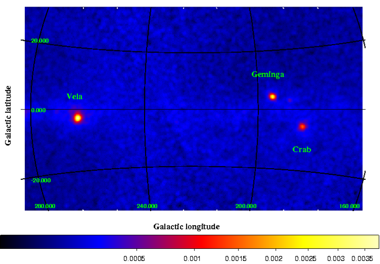
Figure 1.— Gaussian-smoothed AGILE intensity map ($\sim$120° $\times$ 60°, units: ph cm^-2 s^-1 sr^-1, E$>$100 MeV) in Galactic coordinates integrated over the whole observing period (2007 July 13–2008 April 10) and centerd at $l=223\arcdeg$, $b=0\arcdeg$. The AGILE field of view (radius $\sim$60°) can embrace in a single pointing Vela ($l=263.6\arcdeg$, $b=-2.8\arcdeg$), Geminga ($l=195.1\arcdeg$, $b=4.3\arcdeg$) and Crab ($l=184.6\arcdeg$, $b=-5.8\arcdeg$) as well as diffuse emission from the Galactic Disk.

The AGILE Commissioning and Science Verification Phases lasted about seven months from 2007 April 23 to November 30 including also Instrument Time Calibration. On 2007 December 1 baseline nominal observations and a pointing plan started together with the Guest Observer program AO 1. Timing observations suitable for pulsed signal analysis of the Vela pulsar started in mid 2007 July (at orbit 1,146) after engineering tests on the payload.

The Vela region was observed (with optimal exposure efficiency) for $\sim$40 days during the SVP and again for $\sim$30 days in AO 1 pointing number 3 (2008 January 8–February 1). PSR B 1706–44 was within the Vela and Galactic Center pointings for $\sim$30 days during the SVP and for $\sim$45 days during AO 1 pointings numbers 5 and 6 (2008 February 14–March 30). The Anti-center region (including Crab and Geminga) was observed for $\sim$40 days, mostly in 2007 September, and in 2008 April (AO 1 pointing number 7) with the addition of other sparse short Crab pointings for SuperAGILE calibration purposes during the SVP (see Table 1 and Figure 2 for details about targets coverage).

Table 1 Observation parameters of the relevant data subsets (grouped in uniterrupted target observations) for each analyzed pulsar considering for comparison all G+L class events (see text) with $E>100$ MeV observed within 60° from the center of the field of view and extracted within 5° from the pulsar position.

PSR	ObsID	TFIRST	TLAST	$\langle\theta\rangle$	Total Counts	Exposure
		[MJD]	[MJD]	[deg]		[108 cm2 s]
Vela	SVP 1	54,294.552	54,305.510	26.2	6440	1.87
Vela	SVP 2-3-4	54,311.512	54,344.569	40.9	12651	3.26
Vela	SVP 5	54,358.525	54,359.521	41.4	391	0.11
Vela	SVP 6	54,367.525	54,377.521	48.9	1355	0.26
Vela	SVP 8	54,395.554	54,406.501	55.3	113	0.03
Vela	AO 1 2	54,450.540	54,457.157	56.2	564	0.01
Vela	AO 1 2-3	54,464.784	54,480.966	22.1	4726	3.13
Vela	AO 1 3-4	54,492.948	54,505.377	43.2	6293	1.16
Vela	AO 1 4-5-6	54,508.528	54,528.537	43.6	9747	2.22
Vela	AO 1 6	54,546.095	54,561.427	41.7	703	0.17
Vela	total	54,294.552	54,561.427	36.1	42983	12.22
Vela	gamma	54,294.552	54,561.427	36.1	6140	5.28
Geminga	SVP 2	54,308.871	54,314.507	55.0	187	0.06
Geminga	SVP 3	54,324.514	54,335.508	41.3	781	0.24
Geminga	SVP 4-5-6-7	54,344.518	54,351.235	22.2	17823	6.19
Geminga	SVP 8	54,395.520	54,406.504	37.6	1926	0.48
Geminga	AO 1 6	54,528.531	54,529.270	50.7	38	0.01
Geminga	AO 1 6	54,546.093	54,549.428	39.0	132	0.03
Geminga	AO 1 6-7	54,555.514	54,566.5	11.7	4860	2.03
Geminga	total	54,308.871	54,566.5	20.2	25962	9.04
Geminga	gamma	54,308.871	54,566.5	20.2	3874	4.54
Crab	SVP 1-2	54,305.509	54,314.50	50.2	2404	0.58
Crab	SVP 3	54,324.512	54,335.508	28.2	761	.0.32
Crab	SVP 4-5-6-7	54,344.518	54,386.502	23.9	20499	6.41
Crab	SVP 8	54,395.518	54,406.506	45.4	1537	0.32
Crab	AO 1 3-4	54,494.447	54,505.390	55.8	350	0.05
Crab	AO 1 4	54,508.506	54,510.474	54.7	359	0.06
Crab	AO 1 6	54,528.531	54,529.140	46.9	100	0.02
Crab	AO 1 6	54,546.091	54,549.423	41.5	176	0.03
Crab	AO 1 6-7	54,555.516	54,566.5	21.8	4973	1.89
Crab	total	54,305.509	54,566.5	26.1	31159	9.68
Crab	gamma	54,305.509	54,566.5	26.1	4062	4.11
B1706–44	SVP 1	54,294.552	54,305.503	50.9	4641	0.91
B1706–44	SVP 2-3-4	54,311.531	54,322.891	34.5	15657	4.39
B1706–44	SVP 7-8	54,386.524	54,393.752	41.5	5521	1.28
B1706–44	AO 1 2-3	54,470.292	54,480.965	53.7	2169	1.46
B1706–44	AO 1 3	54,492.948	54,497.509	44.9	1507	0.20
B1706–44	AO 1 5-6	54,510.482	54,555.509	22.4	24219	7.36
B1706–44	total	54,294.552	54,555.509	28.7	53714	15.6
B1706–44	gamma	54,294.552	54,555.509	28.7	8463	6.566.56

Figure 2.— Post-fit timing residuals (in milli-turns) as a function of the Modified Julian Day resulting from the observation at 1.4 GHz of the three radio pulsars which are discussed in this paper: from the top Vela, Crab and PSR B1706$-$44. The panels in the left (right) column report the residuals of the best available timing solutions obtained over the data span not including (including) the correction of the timing noise via the use of the $\Delta R$ term (see § 4). Note that for the Crab pulsar the scale on the vertical axis of the panel in the right column is amplified by a factor 10 with respect to that in the left panel. The time intervals corresponding to the useful AGILE pointings for each target are also given as the black sections of the bar at the bottom of each panel.

GRID data of the relevant observing periods were grouped in 20 subsets of 200 orbits each (corresponding to $\sim$15 days of observation) starting from orbit 1,146 (54,294 MJD). Data screening, particle background filtering and event direction and energy reconstruction were performed by the AGILE Standard Analysis Pipeline (BUILD-15) for each subset with an exposure $>$$10^{6}$ cm² s at $E>100$ MeV. Observations affected by coarse pointing, non-nominal settings or intense particle background (e.g. orbital passages in South Atlantic Anomaly) and albedo events from the Earth’s limb were excluded from the processing.

A specific optimization on the events extraction parameters is performed for each target in order to maximize the signal to noise ratio for a pulsed signal. The optimal event extraction radius around pulsar positions varies as a function of photon energy (and then it is related to pulsar spectra) according to the Point Spread Function. However, for $E>100$ MeV broad band analysis, a fixed extraction radius of $\sim$5° (a value slightly higher than the Point Spread Function 68% containment radius) produces comparable results with respect to energy-dependent extraction.

Quality flags define different GRID event classes. The G event class includes events identified with good confidence as photons. Such selection criteria correspond to an effective area of $\sim$250 cm² above 100 MeV (for sources within 30 deg from the center of the field-of-view). The L event class includes events typically affected by an order of magnitude higher particle contamination than G, but yielding an effective area of $\sim$500 cm² at $E>100$ MeV, if grouped with the G class. We performed our timing analysis looking for pulsed signals using both G class events and the combination of G+L events. In general, the signal-to-noise ratio of the pulsed signal is maximized using photons collected within $\sim$40° from the center of GRID field of view and selecting the event class G. For very strong sources, such as Vela, or sources located in low background regions, it is possible to include also photons in the 40–60° off-axis range and belonging to the G+L event class typically improving the count statistics by up to a factor of three (obviously implying also a much higher background), without affecting or even improving the detection significance. For each pulsar, Table 1 summarizes the exposure parameters of the relevant data subsets grouped in uninterrupted target observations. For simplicity and comparison, we reported in Table 1 and Table 2 observation and detection parameters obtained with the same extraction criteria and energy range. For all observations with the targets within 60° from the pointing direction, we list the average angular distance $\langle\theta\rangle$ of the source position from the pointing direction, the sum of all G+L events with $E>100$ MeV whose direction is within 5° from the pulsar position and the G only events (“gamma photons”), selected with the same criteria. The choice to include all G+L events yields a “dirty” data set: for the case of Vela, $\sim$10% of the total counts are ascribable to the Galactic Plane, and $>$50% are particle background ($\sim$10,000 source counts). The contamination is reduced in the “gamma” entry, characterized by $\sim$20% diffuse emission and $\sim$5% particle background ($\sim$5,000 source counts). The corresponding exposure for each data subset was calculated with the GRID scientific analysis task AG_ExpmapGen according with the above parameters. Summing up the photon numbers, we see that the overall photon statistics accumulated (accounting for background contamination) is comparable to that collected by EGRET for the same four pulsars.

Table 2 The photon harvest from the AGILE observations of gamma-ray pulsars.

PSR	P	$\dot{E}$	$d$	Pulsed Counts	$\chi^{2}_{r}$ (d.o.f)	Exposure	Pulsed Flux
	(ms)	(erg s-1)	(kpc)			(108 cm2 s)	10-8 ph. cm-2 s-1
Vela	89.3	$6.92\times 10^{36}$	0.29	$9,170\pm 580$	225.51 (9)	12.22	$940\pm 60$
Geminga	237.1	$3.25\times 10^{34}$	0.16	$2,200\pm 480$	10.44 (9)	9.04	$300\pm 70$
Crab	33.1	$4.61\times 10^{38}$	2.00	$2,120\pm 530$	10.71 (9)	9.68	$270\pm 70$
B1706–44	102.5	$3.41\times 10^{36}$	1.82	$2,370\pm 720$	9.11 (9)	15.6	10$190\pm 60$

Note. — See text for details on data reduction and timing analysis.

A maximum likelihood analysis (ALIKE task) on the AGILE data from the sky areas containing the four gamma-ray pulsars yielded source positions, fluxes and spectra in good agreement with those reported both in the EGRET catalogue for the corresponding 3EG sources (Hartman et al., 1999) and in the revised catalogue by Casandjian & Grenier (2008). As an example, Figure 1 reports an AGILE intensity map displaying Vela, Geminga and Crab. Details on gamma-ray imaging and spectra of the four sources will be reported in future papers when count statistics significantly higher than that currently available are collected and in-flight Calibration files are finalized.

In this paper we focus on timing analysis. However, it is worth noticing that pulsed counts provide a gamma-ray pulsar flux estimate independent from the likelihood analysis, as described in § 5.

3. Radio/X-rays observations and timing

In order to perform AGILE timing calibration through accurate folding and phasing, as described in §§ 4 and 5, pulsar timing solutions valid for the epoch of AGILE observations were required. Thus, a dedicated pulsar monitoring campaign (that will continue during the whole AGILE mission) was undertaken, using two telescopes (namely Jodrell Bank and Nançay) of the European Pulsar Timing Array (EPTA), as well as the Parkes radio telescope of the Commonwealth Scientific and Industrial Research Organisation (CSIRO) Australia Telescope National Facility (ATNF) and the 26m Mt Pleasant radio telescope operated by the University of Tasmania.

In particular, the observations of the Vela Pulsar have been secured by the Mt. Pleasant Radio Observatory. Data were collected at a central frequency of 1.4 GHz. Given the pulsar brightness, it is possible to extract a pulse Time of Arrival (ToA) about every 10 seconds, so that a total of 4,098 ToAs have been obtained for the time interval between 2007 February 26 (MJD 54,157) and 2008 March 23 (MJD 54,548), encompassing the whole time span of the AGILE observations. During this time interval the pulsar experienced a small glitch (fractional frequency increment $\Delta\nu_{g}/\nu\simeq 1.3\times 10^{-9}$), which presumably happened around 2007 August 1 (with an uncertainty of $\pm$3 days due to the lack of observations around this period) (see § 6.3). Ephemeris for the pre- and post-glitch time intervals were then separately calculated and applied to the gamma-ray folding procedure.

The observations of the Crab Pulsar have been provided by the telescopes of Jodrell Bank and Nançay. At Jodrell Bank the Crab Pulsar has been observed daily from 2006 December 09 (MJD 54,078) to 2007 October 06 (MJD 54,379) and again from 2008 February 06 (MJD 54,502) to 2008 April 10 (MJD 54,566) which result in 334 ToAs. The observations were mainly performed at 1.4 GHz with the 76 m Lovell telescope, with some data also taken with the 12-m telescope at a central frequency of 600 MHz. The Nançay Radio Telescope (NRT) is a transit telescope with the equivalent area of a 93 m dish and observed at a central frequency of 1.4 GHz over the time interval between 2006 December 05 (MJD 54,074) and 2007 September 07 (MJD 54,350), producing 64 ToAs. A timing solution was produced by joining the ToAs from the two telescopes and accounting for the phase shift that naturally ensues from data sets coming from different telescopes.

The observations of pulsar B 1706$-$44 have been performed at the 64 m telescope at Parkes, in Australia, at the mean observing frequency of 1.4 GHz. They produced a total of 20 ToAs over the interval from 2007 April 30 (MJD 54,220) to 2008 Apr 6 (MJD 54,562), thus covering the whole AGILE observing time span for this target.

The timing of all pulsars is performed using the TEMPO2 software (Hobbs et al., 2006; Edwards et al., 2006). It first converts the topocentric TOAs to solar-system barycentric TOAs at infinite frequency (using the Jet Propulsion Laboratory [JPL] DE405 solar-system ephemeris) and then performs a multi-parameter least-square fit to determine the pulsar parameters. The differences between the observed barycentric ToAs and those estimated by the adopted timing model are represented by the so-called $residuals$. The procedure is iterative and improves with longer timescales of observations. An important feature developed by TEMPO2 is the possibilty of accounting for the timing noise in the fitting procedure (see § 4). This is particularly useful in timing the young pulsars: in fact most of them suffer of quasi-random fluctuations (typically characterized by a very red noise spectrum) in the rotational parameters, whose origin is still debated. TEMPO2 corrects the effects of the timing noise on the residuals by modeling its behaviour as a sum of harmonically correlated sinusoidal waves (see Equation [2] in § 4) that is subtracted from the residuals.

The left panels (labeled as pre-whitening) in Figure 2 reports the timing residuals obtained over the data span of the radio observations without the correction for the timing noise, whereas the right panels (labeled as whitened) show the residuals after the application of the correction. The comparison between the panels in the two columns shows that this procedure has been very effective in removing the timing noise in Vela, Crab and PSR B1706$-$44. The impact of this whitening procedure on the gamma-ray data analysis is discussed in § 5.

Geminga is a radio-quiet pulsar whose ephemeris can be obtained from X-ray data. Following the demise of CGRO, Geminga was regularly observed with XMM-Newton in order to maintain its ephemeris for use in analyzing observations at other wavelengths. We analyzed all eight observations of Geminga (1E 0630+178, PSR J 0633+1746) taken with the X-ray (0.1–15 keV) cameras of XMM-Newton (Jansen et al., 2001) between MJD 52,368 and MJD 54,534 (2002 April - 2008 March), with exposures in the range 20-100 ks.

The data were processed using version 7.1.0 of the XMM-Newton Science Analysis Software (SAS) and the calibration files released in 2007 August. For the timing analysis we could only use the pn data (operated in Small Window mode: time resolution 6 ms, imaging on a $4\arcmin\times 4\arcmin$ field), owing to the inadequate time resolution of the MOS data. We selected only single and double photon events (patterns 0–4) and applied standard data screening criteria. Photons arrival times were converted to the Solar system barycenter using the SAS task barycen. To extract the source photons we selected a circle of 30$\arcsec$ radius, containing about 85% of the source counts. Using standard folding and phase-fitting techniques, the source pulsations were clearly detected in all the observations. We derived for Geminga the long-term spin parameters valid for the epoch range 52,369-54,534 MJD. Note that the absolute accuracy of the XMM-Newton clock is better than 600 $\mu$s (Kirsch et al., 2004).

The Crab Pulsar is embedded in the Crab Nebula and represents about 10% of its flux in the hard X-ray band. Being a bright source with a relatively soft high-energy spectrum, the Crab pulsar is easily detected by SuperAGILE in less than one AGILE orbital revolution. Since the on-board time reconstruction of SuperAGILE (Feroci et al., 2007) is different from that of the GRID, as a cross-check and test of the SuperAGILE timing performances we processed the X-ray data of an on-axis observation of $\sim$0.7 days (54,360.7–54,361.4 MJD), corresponding to an effective exposure of $\sim$41 ks. In the analysed data the passages of AGILE in the South Atlantic Anomaly and intervals of source occultation by the Earth were excluded. The time entries in SuperAGILE event files are in the on-board time reference system (Coordinated Universal Time) and were converted in Terrestrial Dynamical Time before being processed and analysed by the same procedures used for the GRID (see § 4). A complete analysis of the X-ray observations of Crab with SuperAGILE is beyond the scope of this work: it will be presented in a future paper, as well as the search for the Crab pulsed signal in the AGILE mini-calorimeter data.

4. Gamma-ray timing procedures

In this section we will describe the timing procedures we have adopted. They have been implemented with two aims: to verify the timing performances of AGILE and to maximize the quality of the detection of the four targets.

AGILE on-board time is synchronized to Coordinated Universal Time (UTC) by Global Positioning System (GPS) time sampled at a rate of 1 Hz. Arrival time entries in AGILE event lists files are then corrected to Terrestrial Dynamical Time (TDT) reference system at ground segment level. In order to perform timing analysis, they have also to be converted to Barycentric Dynamical Time (TDB) reference and corrected for arrival delays at Solar System Barycenter (SSB). This conversion is based on the precise knowledge of the spacecraft position in the Solar System frame. To match instrumental microsecond absolute timing resolution level, the required spacecraft positioning precision is $\lesssim$0.3 km. This goal is achieved by the interpolation of GPS position samples extracted from telemetry packets. Earth position and velocity with respect to SSB are then calculated by JPL planetary ephemeris DE405. All the above barycentric corrections are handled by a dedicated program (implemented in the AGILE standard data reduction pipeline) on the event list extracted according to the criteria described in § 2.

Pulsed signals in GRID gamma-ray data cannot be simply found by Fourier analysis of the photon SSB arrival times, since the pulsar rotation frequencies are 4–5 order of magnitude higher than the gamma-ray pulsars typical count-rates (10–100 counts/day). The determination of the pulsar rotational parameters in gamma-ray must then start from an at least approximate knowledge of the pulsar spin ephemeris, provided by observations at other wavelengths.

Standard epoch folding is performed over a tri-dimensional grid centered on the nomimal values of the pulsar spin frequency $\nu_{0}$ and of its first and second order time derivatives, $\dot{\nu_{0}}$ and $\ddot{\nu_{0}},$ as given by the assumed (radio or X–ray) ephemeris at their reference epoch $t_{0}=\rm PEPOCH$. The axes of the grid are explored with steps equal to 1/T${}_{span},$ 2/T${}_{span}^{2}$ and 6/T${}_{span}^{3}$ respectively (all of them oversampled by a factor 20), where T_span is the time span of the gamma-ray data. For any assigned tern $[\nu;~{}\dot{\nu};~{}\ddot{\nu}],$ the pulsar phase $\Phi^{*}$ associated to each gamma-ray photon is determined by the expression:

$$\Phi^{*}=\Phi_{0}+\nu\Delta t+\frac{1}{2}\dot{\nu}\Delta t^{2}+\frac{1}{6}\ddot{\nu}\Delta t^{3}$$ (1)

where $\Delta t=t-t_{0}$ is the difference between the SSB arrival time $t$ of the photon and the reference epoch $t_{0}$ of the ephemeris and $\Phi_{0}$ is a reference phase (held fixed for all the set). A light-curve is formed by binning the pulsar phases of all the photons and plotting them in a histogram. Pearson’s $\chi^{2}$ statistic is then applied to the light-curves resulting from each set of spin parameters, yielding the probabilities of sampling a uniform distribution. These probabilities ${\cal{P}}(\nu;~{}\dot{\nu};~{}\ddot{\nu})$ are then weighted for the number ${\cal{N}}_{\rm st}$ of steps over the grid which has been necessary to reach the set $[\nu;~{}\dot{\nu};~{}\ddot{\nu}]$ starting from $[\nu_{0};~{}\dot{\nu}_{0};~{}\ddot{\nu}_{0}].$ The maximum value over the grid of ${\cal{S}}=1-{\cal{N}}_{\rm st}{\cal{P}}(\nu;~{}\dot{\nu};~{}\ddot{\nu})$ finally determines which are the best gamma-ray rotational parameters for the target source in the surroundings of the given ephemeris. Of course, the higher the value of ${\cal{S}}$, the higher is the statistical significance of a pulsating signal. We note that this approach allows to avoid any arbitrariness in the choice of the range of the parameters to be explored, which otherwise can affect the significance of a detection.

Due to the brightness of the sources discussed in this paper, period folding around the extrapolated pulsar spin parameters obtained from publicly available ephemerides (ATNF Pulsar Catalog, Manchester et al. 2005, and Jodrell Bank Crab ephemeris archive, Lyne et al. 1993) or from recent literature led us to firmly detect ($>$$5\sigma$) the pulsations for all the four targets with a reasonable number of trials ($\stackrel{{\scriptstyle<}}{{{}_{\sim}}}$1,000). However, for three of them (Crab, Vela and PSR B1706$-$44), the best gamma-ray spin period fell outside the $3\sigma$ uncertainty range of the adopted radio ephemeris, and the detection significance ${\cal{S}}$ resulted lower than that derived using contemporary timing solutions (accounting for the effects of timing noise and/or occasional glitches), provided by dedicated radio observation campaigns (see § 3). As expected, for steady and older pulsars, such as Geminga, the availability of contemporary rotational parameters turned out to be less important; even using a few-year-old ephemeris, the pulsed signal could be detected within only $<$100 period search trials around the extrapolated X-ray timing solutions.

An additional significant improvement (see § 5) in the detection significance has been obtained by accounting also for the pulsar timing noise in the folding procedure. This exploits a tool of TEMPO2 (Hobbs et al., 2006; Edwards et al., 2006), namely the possibility of fitting timing residuals with a polynomial harmonic function $\Delta R$ in addition to standard positional, rotational and (when appropriate) binary parameters (Hobbs et al., 2004):

$$\Delta R(\Delta t)=\sum_{k=1}^{N}a_{k}\sin(k\omega\Delta t)+b_{k}\cos(k\omega\Delta t)$$ (2)

where $N$ is the number of harmonics (constrained by precision requirements on radio timing residuals, as well as by the span and the rate of the radio observations), $a_{k}$ and $b_{k}$ are the fit parameters (i.e. the $\it{WAVE}$ terms in TEMPO2 ephemeris files), and $\omega=2\pi(T_{radio}(1+4/N))^{-1}$ is the main frequency (i.e. $\it{WAVE_{OM}}$ in TEMPO2 ephemeris files) related to the radio data time-span $T_{radio}$.

If the spin behavior of the target is suitably sampled, the harmonic function $\Delta R$ can absorb the rotational irregularities of the source, in a range of timescales ranging from $\sim$$T_{radio}$ down to about the typical interval between radio observations. As an example, the peak-to-peak amplitude of the $\Delta R$ fluctuations for Crab related to the radio monitoring epochs (54,074–54,563 MJD) covering our AGILE observations are of the order of $\sim$1 ms, corresponding to a phase smearing $>$0.03, a value significantly affecting the time resolution of a $>$50 bins light-curve. Under the assumption that the times of arrival of the gamma-ray photons are affected by timing noise like in the radio band, gamma-rays folding can properly account for $\Delta R$, extending the relation 1 to:

$$\Phi = \Phi^{*}+(\nu+\dot{\nu}\Delta t+\frac{1}{2}\ddot{\nu}\Delta t^{2})\Delta R$$ (3)

$$\simeq \Phi_{0}+\nu\Delta t(1+\frac{\Delta R}{\Delta t})+\frac{1}{2}\dot{\nu}\Delta t^{2}+\frac{1}{6}\ddot{\nu}\Delta t^{3}$$

As reported in § 5, this innovative phasing technique improves significantly the gamma-ray folding accuracy for young and energetic pulsars, especially when using long data spans, like those of the AGILE observations. Of course, the implementation of this procedure requires radio observations covering the time span of the gamma-ray observations making the radio monitoring described in § 3 all the more important.

5. Timing calibration tests and results

In order to verify the performances of the timing analysis procedure described in § 4, a crucial parameter to check is the difference between pulsar rotation parameters derived from radio, X-ray and gamma-ray data. Figure 3 shows the AGILE period search result for the Crab pulsar (corresponding to the MJD 54,305–54,406 observations, significantly affected by timing noise, as shown in Figure 2). The implementation of the folding method described in section § 4 (including timing noise corrections as given by Equation [3]) allowed for a perfect match between the best period resulting from gamma-ray data and the period predicted by the radio ephemeris with discrepancies $\Delta P_{\rm Crab}\sim 3\times 10^{-12}$ s, comparable to the period search resolution $r_{\rm Crab}\sim 2\times 10^{-12}$ s. This represents also an ultimate test for the accuracy of the on-board AGILE Processing and Data Handling Unit (PDHU; Argan et al., 2004) time management (clock stability in particular) and on-ground barycentric time correction procedure. Standard folding without $\Delta R$ term implies radio-gamma period discrepancies one order of magnitude higher ($\Delta P_{\rm Crab}\sim 4\times 10^{-11}$ s). Moreover, it lowers also the statistical significance of the detection and effective time resolution of the light-curve. For the Crab, the value of the Pearson’s $\chi^{2}$ statistic introduced in § 4 (we quote reduced $\chi^{2}$ values) goes from $\sim$6.3 (when using the $\Delta R$ term) down to $\sim$4.2 (ignoring the $\Delta R$ term) when folding the data into a 50 bins light-curve (see Figure 4). Obviously, ignoring timing noise in the folding process would yield discrepancies (and light curve smearing) which are expected to grow when considering longer observing time span. Thus the contribution of timing noise should be considered both in high-resolution timing analysis and in searching for new gamma-ray pulsars. The same analysis applied to Vela and PSR B 1706–44 – much less affected than Crab by timing noise in the considered data span – led to similar results for the period discrepancies ($\Delta P_{\rm Vela}\sim 8\times 10^{-12}$ s, $\Delta P_{\rm B1706}\sim 3\times 10^{-11}$, to be compared with the period search resolution $r_{\rm Vela}\sim 9\times 10^{-12}$ s and $r_{\rm B1706}\sim 2\times 10^{-11}$ s).

Figure 3.— Period search result for the Crab pulsar (period trials vs. $\chi^{2}$ Pearson statistics). The radio period (vertical line at $P_{\rm trial}-P_{\rm radio}=0$) is 33.607554009(4) ms ($PEPOCH=54,362.242$ MJD). Dashed line is obtained from standard folding period trials, while continuos line is from the folding technique accounting for timing noise (see § 3). The new method allow us to perfectly match the radio period in gamma rays ($P_{\rm gamma\_tn}-P_{\rm radio}\sim 3\times 10^{-12}$ s). It is worth noting that in the considered data span (54,305–54,406 MJD) the period search resolution ($r_{\rm Crab}\sim 2\times 10^{-12}$ s) is about an order of magnitude higher than the 1$\sigma$ error on the radio period.

Figure 4.— The Crab light-curve (50 bin) corresponding to the data span 54,305–54,406 MJD obtained by folding including $\Delta R$ terms compared with that obtained neglecting timing noise (dashed line). In observing periods strongly affected by timing noise, the smearing effects reduce detection significance and observed pulsed counts (see text).

For the radio-quiet Geminga pulsar we used X-ray ephemeris obtained from XMM-Newton data (see § 3) as a starting point for the period search. Due to the stability of the spin parameters of this relatively old pulsar, not significantly affected by timing noise, $\it{WAVE}$ parameters are not required for the folding process. The X-ray versus gamma-ray period discrepancy was $\Delta P_{\rm Gem}\sim 9\times 10^{-12}$ s, whereas $r_{\rm Gem}\sim 7\times 10^{-11}$ s. We here note that the frequency resolution 1/T${}_{\rm span}\sim 10^{-7}$ Hz of AGILE is about one order of magnitude better than that corresponding to a single XMM-Newton exposure (lasting $\stackrel{{\scriptstyle<}}{{{}_{\sim}}}100$ ks), but the few year long X-ray data span implies an overall much better effective resolution 1/T${}_{\rm XMM}\sim 5\times 10^{-9}$ Hz for the XMM-Newton data.

The resulting gamma-ray light-curves, covering different energy ranges for the four pulsars, are shown in Figures 5, 6, 7, and 8. The pulsed flux was computed considering all the counts above the minimum of the light-curve, using the expression $PF=C_{\rm{tot}}-nN_{\rm{min}}$ and its associated error $\sigma_{PF}=(C_{\rm{tot}}+n^{2}\sigma^{2}_{N_{\rm{min}}})^{1/2}\simeq n(N_{\rm{min}})^{1/2}$, where $C_{\rm{tot}}$ are the total counts, $n$ is the number of bins in the light-curve and $N_{\rm{min}}$ are the counts of bin corresponding to the minimum. This method is “bin dependent”, but reasonable different choices of both the number of bins (i.e. $n>10$) and of the location of the bin center (10 trial values were explored for each choice of $n$) do not significantly affect the results. Several models (polar cap, slot gap) predict that gamma-ray pulsar emission is present at all phases. When enough counts statistics will be available, (e.g. $\sim$10,000 counts for the Crab pulsar), it will be possible to estimate the unpulsed emission (due to the pulsar plus a possible contribution from the pulsar wind nebula) by considering the difference among the total source flux obtained by a likelihood analysis on the images and the pulsed flux estimated with the above method.

Figure 5.— Vela pulsar light-curves ($P\sim 89.3$ ms) for different energy bands ($E<100$ MeV, 40 bins, resolution: $\sim$2.2 ms; $E>100$ MeV, 100 bins, resolution: $\sim$0.9 ms; $E>1$ GeV, 20 bins, resolution: $\sim$4.5 ms; G+L class events) obtained by integrating all available post-glitch data (54,320–54,561 MJD). The radio ephemeris and the 8,192 bins light-curve (bottom panel) are obtained by the analysis of $\sim$4,100 ToAs observed at Mt. Pleasant Radio Observatory in Tasmania (radio observation interval 54,157–54,548 MJD).

Figure 6.— Geminga light-curves ($P\sim 237.1$ ms) for different energy bands ($E<100$ MeV, 20 bins, resolution: $\sim$11.8 ms; $E>100$ MeV, 100 bins, resolution: $\sim$2.4 ms; $E>1$ GeV, 20 bins, resolution: $\sim$11.8 ms; G class events). The X-ray ephemeris and the 1–8 keV 40 bins light-curve (bottom panel) are obtained by the analysis of XMM-Newton data (observation interval 52,369–54,534 MJD).

Figure 7.— Crab pulsar light-curves ($P\sim 33.1$ ms) for different energy bands ($E>100$ MeV, 50 bins, resolution: $\sim$0.7 ms; $E>500$ MeV, 40 bins, resolution: $\sim$0.8 ms; G class events) obtained by integrating all available data presented in Table 1. The X-ray (18–60 keV) SuperAGILE 50 bins light-curve is obtained from a $\sim$41 ks observation taken at $\sim$54,361 MJD. The radio ephemeris and the 2048 bins light-curve (bottom panel) are obtained by the analysis of 334 ToAs observed by Jodrell Bank and Nançay radio telescopes (observation interval 54,078–54,566 MJD).

Figure 8.— PSR B 1706–44 light-curves ($P\sim 102.5$ ms) for different energy bands ($E>30$ MeV, G class events, 40 bins, resolution: $\sim$2.6 ms; $0.1<E<1$ GeV, G+L class events, 20 bins, resolution: $\sim$5.1 ms; $E>1$ GeV, G+L class events, 10 bins, resolution: $\sim$10.2 ms) obtained by integrating all available data presented in Table 1. The radio ephemeris and the 1024 bins light-curve (bottom panel) are obtained by the analysis of 20 ToAs observed by Parkes radio telescope (observation interval 54,220–54,562 MJD).

Pulsed counts and related Pearson statistics for the four pulsars are reported in Table 2 (for the standard event extraction parameters as in Table 1). The resulting fluxes (Pulsed Counts/Exposure) are consistent with those reported in the EGRET Catalogue (Hartman et al., 1999). We note that source-specific extraction parameters (event class, source position in the field of view, energy band etc.) which maximize reduced $\chi^{2}$ can significantly improve detection significance. For example, including only event class G in the timing analysis of Crab and Geminga halves the number of pulsed counts while doubling the $\chi^{2}$ values.

Despite the very satisfactory matching of the pulsar spin parameters found in radio (or X-ray) and gamma-ray (supporting the clock stability and the correctness of the SSB transformations), possible systematic time shifts in the AGILE event lists could be in principle affecting phasing and must be checked. For example, an hypothetical constant discrepancy of t_err of the on-board time with respect to UTC would result in a phase shift $\Phi_{err}=(t_{err}~{}\rm{mod}~{}P)/P$, where $P$ is the pulsar period. The availability of radio observations bracketing the time span of the gamma-ray observations (or of X-ray observations very close to the gamma-ray observations for the case of Geminga) allowed us to also perform accurate phasing of multi-wavelength light-curves. In doing that, radio ephemeris reference epochs were set to the main peak of radio light-curves at phase $\Phi_{peak}=0$. In view of Equations (2) and (3), this is achieved by setting $\Phi_{0}=-\nu\sum_{k=1}^{N}b_{k}$ (typically $\Phi_{0}<10^{-2}$). We found that the phasing of the AGILE light-curves of the four pulsars (radio/X-rays/gamma-ray peaks phase separations) is consistent with EGRET measurements (Fierro et al., 1998; Thompson et al., 1996; Jackson & Halpern, 2005, see § 6 for details) implying no evidence of systematic errors in absolute timing with an upper limit $t_{err}<1$ ms.

Comparison with the SuperAGILE light-curve peak (see § 3) is also interesting (SuperAGILE on-board time processing is more complex than that of the GRID). The Crab SuperAGILE light-curve (Figure 7) was produced with the same folding method reported in § 4, yielding $63,700\pm 8,700$ pulsed counts ($\sim$3% of the total counts including background). Inspection of Figure 7 shows that the X-ray peaks are aligned with the $E>100$ MeV data within $\Delta\phi\sim 400$ $\mu$s (a value obtained fitting the peaks with Gaussians) providing an additional test of the AGILE phasing accuracy.

The effective time resolution of AGILE light-curves results from the combination of the different steps involved in the processing of gamma-ray photon arrival times. The on-board time tagging accuracy is a mere $\sim$1 $\mu$s, with negligible dead time. For comparison, the corresponding EGRET time tagging accuracy was $\sim$100 $\mu$s. The precise GPS space-time positioning of AGILE spacecraft (Argan et al., 2004) allows for the transformation from UTC to Solar System barycenter time-frame (TDB) with only a moderate loss ($\lesssim$10 $\mu$s) of the intrinsic instrumental time accuracy. The innovative folding technique described in § 4, accounting for pulsar timing noise, also reduces smearing effects in the light-curves, fully exploiting all the information from contemporary radio observations. In summary, the effective time resolution of the current AGILE pulsar light-curves (and then multi-wavelength phasing accuracy assuming $t_{err}=1$ $\mu$s) is mainly limited by the available count statistics and can be estimated by:

$$\Delta t={{P}\over{N}}={{\sigma^{2}(C_{p}+2B)}\over{C_{p}^{2}}}$$ (4)

where $P$ is pulsar period, $N$ is the number of bins in the light-curve histogram, $\sigma$ is the signal-to-noise ratio, $C_{p}$ are the pulsed counts and $B$ are the background counts. In order to keep the average signal-to-noise ratio of light-curve bins (during the on-pulse phase) at a reasonable level ($>$3 $\sigma$), the resulting effective time resolution is constrained to 200–500 $\mu$s. At present, the best effective time resolution ($\sim$200 $\mu s$) is obtained for the 400-bin light-curve of Vela (G+L class selection) although a 100-bins light-curve (Figure 5) is better suited to study pulse shapes and to search for possible weak features. The effective time resolution will obviously improve with exposure time $\Delta t\propto T_{exp}^{-1}$ and a resolution $\stackrel{{\scriptstyle<}}{{{}_{\sim}}}$50 $\mu$s is expected after two years of AGILE observations of Vela.

6. Discussion

With about 10 years since the last gamma-ray observations of Crab, Vela, Geminga (Fierro et al., 1998) and B 1706–44 (Thompson et al., 1996) by CGRO, the improved time resolution of AGILE and the much longer observation campaigns in progress are now offering the possibility of both to search for new features in the shape of the light-curves of these gamma-ray pulsars and to investigate the possible occurrence of variations in the gamma-ray pulsed flux parameters.

After nine months of observations in the frame of the Science Verification Phase (2007 July–November) and of the Scientific Pointing Program AO 1 (pointings 1–7, 2007 December 1–2008 April 10), AGILE reached an exposure (E$>$100 MeV) of the Vela region $\gtrsim$$10^{9}$ cm² s ($\sim$10,000 pulsed counts from Vela), comparable to that of the nine-year life of EGRET (although AGILE data have a higher residual particle background), and an even better exposure ($1.5\times 10^{9}$ cm² s) in the core region of the Galactic Plane ($l=310\arcdeg$–$340\arcdeg$) corresponding to the Southern Hemisphere . In fact, AGILE observed $\sim$2,400 pulsed counts from PSR B1706$-$44 up to date, a factor 1.5 better counts statistics than EGRET for this source. For Crab and Geminga, an exposure level comparable with that obtained by EGRET will be reached at the end of the AO 1 pointing number 15 in the Anti-Center region (October, 2008).

6.1. The gamma-ray light-curves

The plots shown in Figures 5, 6, 7, and 8 allow us to start assessing new features in gamma-ray pulsar light-curves. Narrower and better resolved main peaks are revealed, together with previously unknown secondary features, to be confirmed when more count statistics (and an improved particle background filtering) will be available.

The Vela light-curves for different energy bands are shown in Figure 5. A Gaussian fit to the Vela main peak (P1) at $E>100$ MeV provides a FWHM of $0.018\pm 0.002$ centered at $\phi=0.1339\pm 0.0007$ in phase consistent with the EGRET observations (Kanbach et al., 1994). The apex of the main peak is resolved by AGILE with a width of $\sim$0.8 ms and its apparent trail ($\phi=0.13$–0.3) could be due to the occurrence of one or more secondary peaks. In fact, marginal evidence of a relatively narrow lower peak (P3) at $\phi\sim 0.25$ is present in the $E<$100 MeV (3.3$\sigma$ fluctuation with respect to the average interpulse rate) and in the $E>$1 GeV (3.8$\sigma$) light-curves. P3 is located at the phase of the optical peak 1, and also at the phase of a bump predicted in a two-pole caustic model (Dyks et al., 2004), due to overlapping field lines from opposite poles near the light cylinder. In the outer gap model, this bump is the first peak in the light-curve, and also comes from very near the light cylinder. The peak at $\phi=0.5$–0.6 (P2) in the $E>100$ MeV light-curve cannot be satisfactorily fit with a single Gaussian or a Lorentzian curve ($\chi^{2}_{r}>3$), due the possible presence of a bump at $\phi\sim 0.5$ (P2a). A fit with two Gaussian provides $\phi=0.560\pm 0.001$ (FWHM $0.031\pm 0.003$) and $\phi=0.49\pm 0.01$ for the phases of the major peak (P2b) and lower peak apex (P2a), respectively. The phase separation between the main gamma-ray peaks $\Delta\phi=0.426\pm 0.002,$ as well as that between the gamma-ray and the radio peak, are unchanged since EGRET observations (Kanbach et al., 1994; Ramanamurthy et al., 1995). In the $E<100$ MeV band a secondary peak+valley structure (P4) appears at $\phi\sim 0.9$ ($\sim$4$\sigma$ level). It is worth noting its symmetric position around the radio peak with respect to main peak (P1) and a possible correlation of P4 with features seen in the X-ray light-curves (Manzali et al., 2007); P4 also coincides with peak number 3 of the RossiXTE light curve (Harding et al., 2002).

Geminga shows an $E>100$ MeV light-curve (Figure 6) with properties similar to those of Vela. Apart from the major peaks P2 ($\phi=0.999\pm 0.002$, FWHM $0.062\pm 0.008$) and P1 (with apex $\phi=0.507\pm 0.004$, FWHM $0.08\pm 0.01$), secondary peaks are seen trailing P1 and leading P2: the main peak’s P2 leading trail ($\phi=0.8$–1) could be possibly associated to unresolved multiple peaks while P1 displays a “bump” at $\phi\sim 0.55$–0.6. P1 seems to be characterized by a double structure: a fit with a simple Gaussian yields $\chi^{2}_{r}\sim 1.2$ to be compared with a double Gaussian model providing $\chi^{2}_{r}<1$. This feature seems still present even considering different observation block separately. The main-peak separation ($\Delta\phi=0.508\pm 0.007$ at $E>100$ MeV) is greater than the value obtained for Vela and it decreases slightly with energy. The 2–10 keV X-ray light-curve shows a peak (P3) in correspondence with a possible excess in the hard gamma-ray band and a broad top-hat shaped feature partially overlapping in phase with P1.

The Crab light-curve for $E>100$ MeV (Figure 7) shows a previously unknown broad feature at $\phi=0.65-0.8$ (P3), in addition to the main peaks P1 and P2 ($\phi_{P1}=0.999\pm 0.002,$ FWHM $0.054\pm 0.005$; $\phi_{P2}=0.382\pm 0.008,$ FWHM $0.14\pm 0.04$). The probability of P3 being a background fluctuation is of $\sim$$10^{-4}$ (3.7$\sigma$). P2 could be possibly resolved in two sub-peaks in future longer observations. P3 is coincident with the feature HFC2 that appears in the radio profile above 4 GHz (Moffett & Hankins, 1996). From the polarization of this component, Moffett & Hankins (1999) suggest that this peak may come from a lower emission altitude, near the polar cap. P3 is actually at a phase that could plausibly come from low altitude cascades in the slot gap model (Muslimov & Harding, 2004, Figure 2), the pairs from which may be also causing the HFC2 radio component(s), while P1 and P2 comes from the high-altitude slot gap.

According to the observations of SAS-2, COS B and CGRO/EGRET, the ratio P2/P1 of the main peak intensities could present a variability pattern (possibly ascribed to the nutation of the neutron star) that can be fit with a sinusoid with a period of $\sim$13.5 years (Kanbach, 1990; Ramanamurthy et al., 1995) although this is not required by EGRET data alone (Tompkins et al., 1997). We observed a P2/P1 intensity ratio $0.66\pm 0.10$ in good agreement with the value of $\sim$0.59 predicted for 54,350 MJD (for the energy range 50 MeV–3 GeV). Unfortunately, our P2/P1 value is similar - within the errors - to the EGRET determination ($\sim$0.5): then an unambiguous assessment of the origin of this possible phenomenology will require measurements close to the epoch (56,150 MJD) corresponding to the predicted maximum or the intensity ratio P2/P1 ($\sim$1.4). Variability should also be invoked to explain the possible detection of P3, which was never seen before in the EGRET database in spite of an overall exposure comparable to that reached by AGILE so far. We note that the main peak intensity ratios computed for Vela ($\rm{P2/P1}=0.91\pm 0.07$) and Geminga ($\rm{P2/P1}=0.8\pm 0.1$) do not yield evidence of significant variations with respect to past observations (Ramanamurthy et al., 1995).

The AGILE light-curves of PSR B 1706$-$44 are shown in Figure 8. The broad-band light-curve ($E>30$ MeV) clearly shows two peaks ($\phi_{P1}=0.211\pm 0.007,$ $\phi_{P2}=0.448\pm 0.005$) bracketing considerable bridge emission (contributing to $>$50% of the pulsed counts) while in the 0.1–1 GeV range the peaks cannot be discerned from the bridge emission and the pulsar profile presents an unresolved broad ($\Delta\phi=0.3-0.4$) single peak. PSR B 1706–44 is a young ($\sim 2\times 10^{4}$ yr) and energetic ($3.4\times 10^{36}$ erg s^-1) 102.5 ms pulsar (Johnston et al., 1992) with emission properties similar to Vela (Becker & Pavlov, 2002). Double peaked PSR B 1706–44 is then in fact “Vela-like” not only energetically, but also with respect to the offset between the maxima of the high energy and the radio profiles, with neither of the two gamma-ray narrow pulses aligned to the radio peak.

AGILE allowed for a long monitoring of gamma-ray pulsar light-curves shapes. We carefully looked for possible lightcurve variations by KS tests (two-dimensional Kolmogorof-Smirnoff test [KS]; Peacock 1983; Fasano & Franceschini 1987). For each pulsar, different gamma-ray light-curves (with 10, 20 and 40 bins) were obtained grouping contiguous data set and requiring at least 30 counts bin^-1 (300–1000 counts for each light-curve). Each light-curve was compared by KS test with each other and with the average shape corresponding to the entire data set. No pulse shape variation was detected with a significance $>$3 $\sigma$ on timescales ranging from 1 days (Vela) to few months (Crab, Geminga and PSR B 1706$-$44).

6.2. Implications for the emission models

Pulsars derive their emitting power from rotational energy loss owing to the relativistic acceleration (up to Lorentz factor $\Gamma\sim 10^{5}$–$10^{7}$) of charged particles by very high electric potentials induced by the rotating magnetic fields. The charge density that builds up in a neutron star magnetosphere is able to short out the electric field parallel to the magnetic field everywhere except a few locations of non-force-free “gaps”. It is unclear whether these acceleration regions can form in the strong field near ($\lesssim$1 stellar radii) the neutron star surface (polar cap/low-altitude slot gap model: Daugherty & Harding (1996) and Muslimov & Harding (2003); high-altitude slot gap model: Muslimov & Harding (2004) and Harding et al. (2008)), in the outer magnetosphere near the speed of light cylinder (outer gap model: Cheng et al. (1986); Romani (1996); Hirotani & Shibata (2001); Takata & Chang (2007)) or even beyond in the wind zone (Pétri & Kirk, 2005).

In polar cap/low altitude slot gap models, gamma-rays result from magnetic pair cascades induced by curvature or inverse-Compton photons. The spectrum is dominated by synchrotron radiation of pairs at lower energies ($\lesssim$1 GeV) and by curvature radiation at higher energies ($>$1 GeV). In the high-altitude slot gap, gamma-rays result from curvature radiation and synchrotron radiation of primary electrons (no cascade). In outer gap models, gamma-rays result from photon-photon pair cascades induced by curvature radiation. The spectrum is dominated by pair synchrotron radiation below 20 MeV, curvature radiation above 20 MeV and inverse Compton at 1–10 TeV.

The size and spectrum of the emitting regions are then directly related to the intensity and location in the magnetosphere of the accelerating electric fields. Strong fields imply thin accelerator gaps, while weaker fields are associated to thick gaps: the acceleration zone grows bigger as the particle must accelerate over larger distance to radiate pair-production photons. On an observational point of view, it is in turn expected that acceleration gap sizes are related to the width of light-curve peaks. The highly relativistic particles emit photons at very small ($\sim$$1/\Gamma$) angles to the open magnetic field lines. The theoretical width of a light-curve peak associated to an infinitely small gap would be then $\Delta t=P/(2\pi\Gamma)$, a value typically smaller than 1 $\mu$s. Therefore, the width of the apex of the peak can be related to the core gap size. For example, the $\Delta t\sim 800$ $\mu$s width of the Vela pulsar peak (P1) resolved by AGILE implies a projected gap core width of $\sim$1 km for gap height of $\sim$1 stellar radii. Broader peaks as P2 and P3 in the Crab light-curve involves instead magnetospheric region tens of kilometers long. The relation of the width of the peaks to the acceleration gap size works for the low altitude emission models but is complicated by relativistic effects (aberration, retardation) in the high-altitude emission models, where the peaks are formed by caustics (Dyks & Rudak, 2003). The peak widths will still depend on the width of the acceleration (outer or slot) gap, but one must perform a comparison with detailed models to constrain the physical size of the gap.

The likely presence of multiple contiguous peaks as P2a-b in the Vela light-curve, P1 in Geminga and possibly within the wide P2 broad peak in Crab could be related to short-term oscillation of gap locations. Light-curve variations on timescales $\gtrsim$1 days are anyway excluded by the KS tests described above. Alternatively, the apparent superimposition of different gaps placed at different heights in the magnetosphere could be another plausible explanation for multiple-contiguous peaks, while the hypothesis of jumps in the acceleration electric fields strength would lack of evident physical justification. In general, the presence of multiple (contiguous or not) structures in the light-curves is difficult to fit in a scenario alternatively involving polar cap, outer gap or wind zone models exclusively. The particle acceleration may well be simultaneously occurring in all the regions predicted by these models. Indeed, a three peak light-curve can still be explained invoking polar cap gaps alone provided that both polar caps can cross the line-of-sight.

Wherever in the magnetosphere a gap can form, a multi-frequency emission may occur along an hollow cone (due to magnetosphere symmetries) or any other suitable surface: light-curve peaks are generated when the viewing angle from any given location on this surface to the observer also crosses the gap. The pulse spectrum slope depends on the accelerating field as well as on the magnetic fields, which strongly affect the synchrotron emission efficiency and the pair attenuation along the cascade path: the stronger the magnetic field is, the steeper the spectrum is. An outer gap can in principle generate pulse spectra extending up to tens of GeV (Zhang & Cheng, 2000), while gaps close to surface high magnetic fields can produce steep spectra (photon index $\lesssim$3; Ramanamurthy et al., 1996) and cut-off in the tens of MeV range (PSR 1509–58, Harding et al., 1997). The absence of corresponding gamma-ray pulse in phase with radio main peaks in Vela and PSR B 1706–44 could be then ascribed to gap-dependent spectral slope and not only to beam angle and viewing geometry differences.

The multiplicity and variety of features seen in AGILE light-curves can pave the way to a parameterized standard model (e.g. with adjustable accelerating electric fields strength, and location in the magnetosphere) for pulsars gaps and their corresponding observed high-energy pulses. In this perspective, the AGILE light-curves time resolution, currently limited only by the (continuously increasing) source counts statistics, will eventually yield a pulsar gaps map by coupling timing analysis and phase resolved spectral analysis.

6.3. The Vela glitch of August 2007

During early AGILE observations, Vela experienced a weak glitch clearly detected in radio as a discontinuity in the pulsar’s spin parameters.

Glitches are small ($\Delta\nu/\nu\sim 10^{-9}$–$10^{-6}$) and sudden ($\lesssim$1 day) discontinuous increases in the pulsar frequency, often followed by a recovery (1–100 days) to the pre-glitch frequency. About $\sim$6% of pulsars are known to have shown glitches), with a higher incidence of events in younger pulsars. This phenomenon is potentially a very promising tool for probing the physics of the neutron star interiors (Lyne et al., 2000). Although no general consensus has been reached to date about the origin of the glitches, many models are based on the exchange of angular momentum between the superfluid neutron star core and its normal, solid crust (Ruderman, 1976, 1991; Alpar et al., 1984b, a). This angular momentum transfer may excite starquake waves, propagating toward the neutron star surface. Since the magnetic field frozen in the crust is “shaken”, the resulting oscillating electromagnetic potential could generate strong electric fields parallel to the magnetic field, which in turn would accelerate particles to relativistic energies, possibly emitting a burst of high-energy radiation.

Since the first observation of a pulsar glitch in 1969 (Radhakrishnan & Manchester, 1969), Vela has shown $\sim$10 major glitches. Due to its large field of view, the quest for possible gamma-ray bursting behavior due to a glitch is then an effective opportunity for AGILE. Despite the fact that the August 2007 glitch is a weak one ($\Delta\nu/\nu\sim 10^{-9}$), it is worthwhile to search for a signal in the AGILE data.

The characteristic energy of a pulsar glitch can be roughly estimated from the associated pulsar frequency jump $E_{\rm glitch}=\Delta E_{\rm rot}=4\pi^{2}I\nu\Delta\nu$, where $I$ ($\sim$10⁴⁵ g cm²) is the neutron star momentum of inertia. The corresponding expected gamma-ray counts would be:

$$C_{\gamma}^{\rm glitch}=\eta{{E_{\rm glitch}A_{\rm eff}}\over{4\pi d^{2}E_{\gamma}}}\simeq 10^{11}\eta{\Delta\nu\over\nu}$$ (5)

where $\eta=[0,1]$ is the unknown conversion efficiency of the glitch energy to gamma-ray emission, $d$ ($\sim$0.3 kpc) is the pulsar distance, $E_{\gamma}$ ($\sim$300 MeV) is the average gamma-ray photon energy assuming a spectral photon index $\Gamma=-2$, and A_eff is the AGILE effective area.

Even in the virtual limit assumption that the entire glitch energy could be driven into gamma-ray emission, a weak glitch with a frequency shift of ${\Delta\nu/\nu}=1.3\times 10^{-9},$ as that observed in August 2007, cannot produce a strong signal ($C_{\gamma}^{\rm glitch}<100$–200 counts), if the core fluence is spread in $\sim$1 day. In fact, no excess on daily timescales was detected, although for much shorter timescales of 3–6 minutes a $>$5 $\sigma$ excess ($\sim$15 counts) in the photon counts is seen at $\sim$54,312.693 MJD (Figure 9).

Figure 9.— Unfolded Vela pulsar light-curve (4.5 min binsize, $E>50$ MeV, G-class events). Dashed lines bracket glitch epoch uncertainty range ($54,313\pm 3$ MJD). A $>$5$\sigma$ count excess at $\sim$54,312.693 MJD could be associated to gamma-ray bursting emission from the glitch.

On the other hand, stronger Vela glitches, as that of 1988 Christmas (McCulloch et al., 1990) with a frequency shift of ${\Delta\nu/\nu}=2\times 10^{-6}$, could in principle produce more significant transient gamma-ray emission. Typical count-rate from Vela is $\sim$100–200 counts day^-1, then a fluence of $\gtrsim$1000 counts in $\sim$1-day or less from the hypothetical gamma-ray glitch burst should be easily detectable. According to Equation (5), such a flux could arise from a glitch with ${\Delta\nu/\nu}\sim 10^{-7}$ (typical Vela glitch size), converting a relatively small fraction ($\eta\sim 0.1$) of its energy in gamma-rays. The chance occurrence of a strong Vela glitch in the AGILE field of view over three years of mission operations is of $\sim$20%.

7. Conclusions

AGILE collected $\sim$15,000 pulsed counts from known gamma-ray pulsars during its first 9 months of operations. The AGILE PDHU clock stability, coupled with the exploitation of pulsar timing noise information, allows for pulsar period fitting with discrepancies with respect to radio measurements at the level of the period search resolution ($\sim$$10^{-12}$ s) over the long gamma-ray data span ($>$6 months). Thanks to AGILE GPS-based high time tagging accuracy ($\sim$1 $\mu$s), the effective time resolution of AGILE light-curves is limited only by the count statistics at current level of exposure ($\sim$$1.2\times 10^{9}$ cm² s for the Vela region). The best effective time resolution obtained for Vela observations is of $\sim$200 $\mu$s for a signal-to-noise $>$3 $\sigma$ in the on-pulse light-curve bins. An improved effective time resolution $\lesssim$ 50$\mu$s is expected after three years of AGILE observations.

AGILE multi-wavelength phasing of the four gamma-ray pulsars is consistent with the results obtained by EGRET, although the high resolution AGILE light-curves show narrower and structured peaks and new interesting features. In particular, a third peak is possibly detected at $\sim$3.7$\sigma$ level in the Crab light-curve and several interesting features seem present in the Vela light-curves.

In any case, the highly structured light-curves hint at a complex scenario for the sites of particle acceleration in the pulsar magnetospheres, implying different electric gaps with physical properties probably mostly related to their height above the neutron star surface. Alternatively, slight spatial oscillations of the gap locations on timescales $\stackrel{{\scriptstyle<}}{{{}_{\sim}}}$1 day could be invoked to explain the multiple contiguous peaks seen in the light-curves.

The foreseen balance of count statistics at the end of AO 1 observing program will allow for phase-resolved spectral analysis of the light-curves and, correspondingly, a spatial mapping of the magnetospheric gaps (their altitude above the neutron star surface being possibly related to the shape of their spectra).

We finally note that the timing calibration and tests presented in this paper pave the way to an effective search for new gamma-ray pulsars with AGILE. The negligible discrepancies among the radio and the gamma-ray pulsar spin parameters seen in the known gamma-ray pulsars imply that the direct folding of the AGILE data on new pulsar candidates is a safe and efficient procedure, when the folding parameters are obtained from radio/X-rays ephemeris having suitable epoch range of validity. In fact, gamma-ray period search trials around radio/X-rays solutions will be unnecessary when simultaneous ephemeris are available, strongly improving the detection significance for faint sources. According to the predicted gamma-ray pulsar luminosities ($L_{\gamma}\propto\dot{E}^{1/2}/d^{2}$, e.g. Pellizzoni et al. 2004), the detection with AGILE of top-ranked Vela-like pulsars is then expected as soon as exposure levels $\gtrsim$$10^{9}$ cm² s ($E>100$ MeV) will be attained for clean G-class events.

References

- Alpar et al. (1984a) Alpar, M. A., Anderson, P. W., Pines, D., & Shaham, J. 1984a, ApJ, 278, 791
- Alpar et al. (1984b) Alpar, M. A., Pines, D., Anderson, P. W., & Shaham, J. 1984b, ApJ, 276, 325
- Argan et al. (2004) Argan, A. et al., 2004, in Nuclear Science Symposium Conference Record, 2004 IEEE, Vol. 1, 371
- Barbiellini et al. (2001) Barbiellini, G., Bordignon, G., Fedel, G., Liello, F., Longo, F., Pontoni, C., Prest, M., & Vallazza, E. 2001, in AIP Conf. Series, Vol. 587, Gamma 2001: Gamma-Ray Astrophysics, ed. S. Ritz, N. Gehrels, & C. R. Shrader, 754
- Becker & Pavlov (2002) Becker, W. & Pavlov, G. G. 2002, preprint (astro-ph/0208356)
- Casandjian & Grenier (2008) Casandjian, J.-M. & Grenier, I. A. 2008, preprint (astro-ph/0806.0113)
- Cheng et al. (1986) Cheng, K. S., Ho, C., & Ruderman, M. 1986, ApJ, 300, 500
- Costa et al. (2001) Costa, E. et al. 2001, X-ray Astronomy: Stellar Endpoints, AGN, and the Diffuse X-ray Background, 599, 582
- Daugherty & Harding (1996) Daugherty, J. K. & Harding, A. K. 1996, ApJ, 458, 278
- Dyks et al. (2004) Dyks, J., Harding, A. K., & Rudak, B. 2004, ApJ, 606, 1125
- Dyks & Rudak (2003) Dyks, J. & Rudak, B. 2003, ApJ, 598, 1201
- Edwards et al. (2006) Edwards, R. T., Hobbs, G. B., & Manchester, R. N. 2006, MNRAS, 372, 1549
- Fasano & Franceschini (1987) Fasano, G. & Franceschini, A. 1987, MNRAS, 225, 155
- Feroci et al. (2007) Feroci, M. et al. 2007, Nuclear Instruments and Methods in Physics Research A, 581, 728
- Fierro et al. (1998) Fierro, J. M., Michelson, P. F., Nolan, P. L., & Thompson, D. J. 1998, ApJ, 494, 734
- Harding et al. (1997) Harding, A. K., Baring, M. G., & Gonthier, P. L. 1997, ApJ, 476, 246
- Harding et al. (2007) Harding, A. K., Grenier, I. A., & Gonthier, P. L. 2007, Ap&SS, 309, 221
- Harding et al. (2008) Harding, A. K., Stern, J. V., Dyks, J., & Frackowiak, M. 2008, ApJ, 680, 1378
- Harding et al. (2002) Harding, A. K., Strickman, M. S., Gwinn, C., Dodson, R., Moffet, D., & McCulloch, P. 2002, ApJ, 576, 376
- Hartman et al. (1999) Hartman, R. C. et al. 1999, ApJS, 123, 79
- Hirotani & Shibata (2001) Hirotani, K. & Shibata, S. 2001, MNRAS, 325, 1228
- Hobbs et al. (2004) Hobbs, G., Lyne, A. G., Kramer, M., Martin, C. E., & Jordan, C. 2004, MNRAS, 353, 1311
- Hobbs et al. (2006) Hobbs, G. B., Edwards, R. T., & Manchester, R. N. 2006, MNRAS, 369, 655
- Jackson & Halpern (2005) Jackson, M. S. & Halpern, J. P. 2005, ApJ, 633, 1114
- Jansen et al. (2001) Jansen, F. et al. G. 2001, A&A, 365, L1
- Johnston et al. (1992) Johnston, S., Lyne, A. G., Manchester, R. N., Kniffen, D. A., D’Amico, N., Lim, J., & Ashworth, M. 1992, MNRAS, 255, 401
- Johnston et al. (1995) Johnston, S., Manchester, R. N., Lyne, A. G., Kaspi, V. M., & D’Amico, N. 1995, A&A, 293, 795
- Kanbach (1990) Kanbach, G. 1990, in The Energetic Gamma-Ray Experiment Telescope (EGRET) Science Symposium, ed. C. E. Fichtel, S. D. Hunter, P. Sreekumar, & F. W. Stecker, 101–113
- Kanbach et al. (1994) Kanbach, G. et al. 1994, A&A, 289, 855
- Kaspi et al. (2000) Kaspi, V. M., Lackey, J. R., Mattox, J., Manchester, R. N., Bailes, M., & Pace, R. 2000, ApJ, 528, 445
- Kirsch et al. (2004) Kirsch, M. G. F. et al. 2004, in X-Ray and Gamma-Ray Instrumentation for Astronomy XIII. Edited by Flanagan, Kathryn A.; Siegmund, Oswald H. W. Proceedings of the SPIE. SPIE, Bellingham WA, ed. K. A. Flanagan & O. H. W. Siegmund, 85–95
- Kramer et al. (2003) Kramer, M. et al. 2003, MNRAS, 342, 1299
- Kuiper et al. (2002) Kuiper, L., Hermsen, W., Verbunt, F., Ord, S., Stairs, I., & Lyne, A. 2002, ApJ, 577, 917
- Kuiper et al. (2000) Kuiper, L., Hermsen, W., Verbunt, F., Thompson, D. J., Stairs, I. H., Lyne, A. G., Strickman, M. S., & Cusumano, G. 2000, A&A, 359, 615
- Labanti et al. (2006) Labanti, C. et al. 2006, in Space Telescopes and Instrumentation II: Ultraviolet to Gamma Ray. Edited by Turner, Martin J. L.; Hasinger, Günther. Proceedings of the SPIE, Volume 6266, pp. 62663Q (2006).
- Lyne et al. (1993) Lyne, A. G., Pritchard, R. S., & Graham-Smith, F. 1993, MNRAS, 265, 1003
- Lyne et al. (2000) Lyne, A. G., Shemar, S. L., & Smith, F. G. 2000, MNRAS, 315, 534
- Manchester et al. (2005) Manchester, R. N., Hobbs, G. B., Teoh, A., & Hobbs, M. 2005, AJ, 129, 1993
- Manchester et al. (2001) Manchester, R. N., Lyne, A. G., Camilo, F., Bell, J. F., Kaspi, V. M., D’Amico, N., McKay, N. P. F., Crawford, F., Stairs, I. H., Possenti, A., Kramer, M., & Sheppard, D. C. 2001, MNRAS, 328, 17
- Manzali et al. (2007) Manzali, A., De Luca, A., & Caraveo, P. A. 2007, ApJ, 669, 570
- McCulloch et al. (1990) McCulloch, P. M., Hamilton, P. A., McConnell, D., & King, E. A. 1990, Nature, 346, 822
- Moffett & Hankins (1996) Moffett, D. A. & Hankins, T. H. 1996, ApJ, 468, 779
- Moffett & Hankins (1999) —. 1999, ApJ, 522, 1046
- Muslimov & Harding (2003) Muslimov, A. G. & Harding, A. K. 2003, ApJ, 588, 430
- Muslimov & Harding (2004) —. 2004, ApJ, 606, 1143
- Peacock (1983) Peacock, J. A. 1983, MNRAS, 202, 615
- Pellizzoni et al. (2004) Pellizzoni, A., Chen, A., Conti, M., Giuliani, A., Mereghetti, S., Tavani, M., & Vercellone, S. 2004, Advances in Space Research, 33, 625
- Perotti et al. (2006) Perotti, F., Fiorini, M., Incorvaia, S., Mattaini, E., & Sant’Ambrogio, E. 2006, Nuclear Instruments and Methods in Physics Research A, 556, 228
- Pétri & Kirk (2005) Pétri, J. & Kirk, J. G. 2005, ApJ, 627, L37
- Prest et al. (2003) Prest, M., Barbiellini, G., Bordignon, G., Fedel, G., Liello, F., Longo, F., Pontoni, C., & Vallazza, E. 2003, Nuclear Instruments and Methods in Physics Research A, 501, 280
- Radhakrishnan & Manchester (1969) Radhakrishnan, V. & Manchester, R. N. 1969, Nature, 222, 228
- Ramanamurthy et al. (1995) Ramanamurthy, P. V., Bertsch, D. L., Fichtel, C. E., Kanbach, G., Kniffen, D. A., Mayer-Hasselwander, H. A., Nolan, P. L., Sreekumar, P., & Thompson, D. J. 1995, ApJ, 450, 791
- Ramanamurthy et al. (1996) Ramanamurthy, P. V., Fichtel, C. E., Kniffen, D. A., Sreekumar, P., & Thompson, D. J. 1996, ApJ, 458, 755
- Romani (1996) Romani, R. W. 1996, ApJ, 470, 469
- Romani & Yadigaroglu (1995) Romani, R. W. & Yadigaroglu, I.-A. 1995, ApJ, 438, 314
- Ruderman (1976) Ruderman, M. 1976, ApJ, 203, 213
- Ruderman (1991) —. 1991, ApJ, 366, 261
- Takata & Chang (2007) Takata, J. & Chang, H.-K. 2007, ApJ, 670, 677
- Tavani et al. (2006) Tavani, M. et al. 2006, in Space Telescopes and Instrumentation II: Ultraviolet to Gamma Ray. Edited by Turner, Martin J. L.; Hasinger, Günther. Proceedings of the SPIE, Volume 6266, pp. 626603 (2006).
- Thompson (2004) Thompson, D. J. 2004, in Astrophysics and Space Science Library, Vol. 304, Cosmic Gamma-Ray Sources, ed. K. S. Cheng & G. E. Romero, 149
- Thompson et al. (1996) Thompson, D. J. et al. 1996, ApJ, 465, 385
- Tompkins et al. (1997) Tompkins, W. F., Jones, B. B., Nolan, P. L., Kanbach, G., Ramanamurthy, P. V., & Thompson, D. J. 1997, ApJ, 487, 385
- Yadigaroglu & Romani (1995) Yadigaroglu, I.-A. & Romani, R. W. 1995, ApJ, 449, 211
- Zhang & Cheng (2000) Zhang, L. & Cheng, K. S. 2000, A&A, 363, 575