Momentum average approximation for models with electron-phonon coupling dependent on the phonon momentum

Abstract

We generalize the momentum average (MA) approximation to study the properties of models with $g_{\mathbf{q}}$ momentum-dependent electron-phonon coupling. As in the case of the application of the original MA to the Holstein model, the results are analytical, numerically trivial to evaluate, exact for both zero bandwidth and for zero electron-phonon coupling, and are accurate everywhere in parameter space. Comparison with available numerical data confirms this accuracy. We then show that further improvements can be obtained based on variational considerations, using the one-dimensional breathing-mode Hamiltonian as a specific example. For example, by using this variational MA, we obtain ground state energies within at most 0.3% error of the numerical data.

I Introduction

There is considerable need to understand the coupling of a particle to its environment, in particular the interaction between a charge carrier and phonons. The physics of polarons – electrons dressed by phonon clouds – is believed to be relevant in explaining a plethora of physical systems and properties, for example in polymers, nanotubes, C₆₀ and other fullerenes,hengsberger ; gunnarsson ; su manganites,salamon Bechgaard salts,mila ; magna and even, possibly, the kink in the quasiparticle dispersion in cuprates, a necessary ingredient for the full understanding of high-temperature superconductivity.lanzara ; shen ; mishchenko ; cuk

It is of obvious benefit to have highly accurate analytical approximations that can be applied to complicated many-body problems, such as the polaron problem. Unfortunately, most existing approximations fail to reproduce the correct physics in “intermediate” regimes where the relevant physics often occurs. In recent worksberciu1 ; goodvin ; berciu3 ; berciu2 ; covaci ; covaci2 we have proposed the so-called momentum average (MA) approximation for calculating the Green’s function of a dressed particle, focusing on the case of an electron dressed by phonons. This approximation is analytical, easy-to-use, and highly accurate throughout all of parameter space, both at low and at high-energies. Its underlying idea is to sum all of the diagrams in the diagrammatical expansion of the self-energy, but with the diagrams approximated in such a way that the full summation can be performed. At the simplest level, this is achieved by replacing all of the free propagators appearing in the self-energy by their momentum average. For the Holstein model, the resulting MA self-energy exhibits not only the exact asymptotic behaviour for zero coupling and zero bandwidth, but it is also in excellent agreement with numerical results in the intermediate regimes where other approximate methods completely fail.berciu1 ; goodvin ; berciu2

In Refs. berciu1, and goodvin, we presented a detailed account of the derivation and application of the simplest-level MA approximation (now known as MA⁽⁰⁾) to the Holstein model, including extensive comparisons to the available numerical data. We further justified the accuracy of the approximation by looking at the spectral weight sum rules. The MA⁽⁰⁾ approximation satisfies the first six spectral weight sum rules exactly, and is highly accurate for all higher order sum rules. In Ref. goodvin, we also pointed out the three key limitations of the MA⁽⁰⁾ approximation: (i) it fails to correctly predict the so-called electron+phonon continuum that must occur at a phonon energy above the ground state energy of the polaron, (ii) its accuracy worsens for small phonon energies, and (iii) the MA⁽⁰⁾ self-energy is independent of momentum.

These shortcomings motivated the systematic improvement of the MA approximation, presented in Ref. berciu2, . This lead to a hierarchy of increasingly more accurate approximations, which we call MA⁽⁰⁾, MA⁽¹⁾, MA⁽²⁾, etc. The increased accuracy is a result of fewer approximations for the self-energy diagrams, however done in such a way that we can still sum all the resulting diagrams analytically. It is also possible to understand the MA approximations in a variational context, as detailed below. From this point of view, the systematic improvements are obtained by including additional states required to reproduce correctly the electron+phonon continuum. In the process we also obtain a momentum-dependent self-energy and higher accuracy throughout all of parameter space, particularly for small phonon energies. As a result, the MA approximations allow us to understand very accurately the Holstein polaron physics, throughout the parameter space, for all energies and momenta.

In this paper we generalize this powerful set of approximations to a much broader class of models with electron-phonon coupling that depends on the phonon momentum. We first derive a simple generalization, leading to what we will continue to call the MA⁽⁰⁾, MA⁽¹⁾, MA⁽²⁾, etc. hierarchy. These are very easy to apply to any Hamiltonian of this class, however while still asymptotically exact for both weak and strong coupling, at intermediary couplings the relative errors are of a few percent. In other words, these can be used to get a quick estimate of typical energies and spectra. We then show how these can be significantly improved, using variational considerations. This generates a second hierarchy of approximations which we call MA^(v,0), MA^(v,1), MA^(v,2), etc., with relative errors well below one percent. As a test case to gauge these accuracies, we use the one-dimensional (1D) breathing-mode Hamiltonian, where high-accuracy numerical results have recently become available.lau

The general electron-phonon coupling model that we consider has the following form in momentum space:

$${\cal H}=\sum_{\mathbf{k}}\varepsilon_{\mathbf{k}}c_{\mathbf{k}}^{\dagger}c_{\mathbf{k}}+\Omega\sum_{\mathbf{q}}b_{\mathbf{q}}^{\dagger}b_{\mathbf{q}}+\sum_{\mathbf{k},\mathbf{q}}\frac{g_{\mathbf{q}}}{\sqrt{N}}c_{\mathbf{k}-\mathbf{q}}^{\dagger}c_{\mathbf{k}}\left(b_{\mathbf{q}}^{\dagger}+b_{-\mathbf{q}}\right).$$ (1)

The first term is the kinetic energy of the electron, where $c_{\mathbf{k}}^{\dagger}$ and $c_{\mathbf{k}}$ are electron creation and annihilation operators, and $\varepsilon_{\mathbf{k}}$ is the electron dispersion. For the single electron (polaron) problem of interest to us, the spin of the electron is irrelevant and we suppress its index. The second term describes a branch of optical phonons of energy $\Omega$, $b_{\mathbf{q}}^{\dagger}$ and $b_{\mathbf{q}}$ being the phonon creation and annihilation operators. The last term describes the coupling of the electron to the phonons, where $g_{\mathbf{q}}$ is the momentum-dependent coupling. Sums are over all momenta inside the first Brillouin zone, and we set $\hbar=1$ and $a=1$ throughout this paper. This general Hamiltonian covers complicated electron-phonon couplings such as those found in the Rashba-Pekkar,rashba ; dykman Fröhlich,frohlich and breathing-modeslezak ; lau models, and it reduces to the Holstein model when $g_{\mathbf{q}}$ is simply a constant.holstein

The quantity of interest to us is the (retarded) single polaron Green’s function:berciu1 ; goodvin

$$G(\mathbf{k},\omega)=\langle 0|c_{\mathbf{k}}\hat{G}(\omega)c_{\mathbf{k}}^{\dagger}|0\rangle=\langle 0|c_{\mathbf{k}}{1\over\omega-{\cal H}+i\eta}c_{\mathbf{k}}^{\dagger}|0\rangle,$$ (2)

where $|0\rangle$ is the vacuum, $c_{\mathbf{k}}|0\rangle=b_{\mathbf{q}}|0\rangle=0$, and $\eta>0$ is infinitesimally small. The importance of this Green’s function is obvious in the Lehmann representation:mahan

$$G(\mathbf{k},\omega)=\sum_{\alpha}\frac{|\langle\alpha|c_{\mathbf{k}}^{\dagger}|0\rangle|^{2}}{\omega-E_{\alpha}+i\eta},$$ (3)

where $\{|\alpha\rangle\}$ and $\{E_{\alpha}\}$ are the complete set of one-particle eigenstates and eigenenergies, ${\cal H}|\alpha\rangle=E_{\alpha}|\alpha\rangle$. In this representation it is clear that the poles of the Green’s function give the one-particle spectrum, and the associated residues, sometimes called quasiparticle (qp) weights, give partial information on the nature of the eigenstates. Knowledge of this Green’s function also allows us to calculate other relevant quantities such as the effective mass of the polaron, the average number of phonons in the polaronic cloud,berciu1 ; goodvin or more detailed phonon numbers statistics.berciu4 Furthermore, its imaginary part is directly measured experimentally by angle-resolved photoemission spectroscopy (ARPES).damascelli

In this paper we will use the 1D breathing-mode Hamiltonian as an example, however, we stress that the methods we present are applicable to any Hamiltonian like Eq. (1) in any dimension. The reason for choosing the 1D breathing-mode Hamiltonian is two-fold. First, in its full 2D form, it describes lattice vibrations in a CuO₂-like plane, where the motion of the O ions living on the bonds connecting the Cu sites is the most important vibrational degree of freedom,lau making it possibly relevant for the study of high-T_c superconductors. The second reason is that exact diagonalization (ED) resultslau have recently become available for its 1D analog, relevant for CuO chains. We focus here on this 1D breathing-mode model because these results serve as an excellent gauge of the accuracy of the generalized MA approximations. Their availability is very fortunate because although there are many numerical results for the Holstein model, it is only due to recent advancements in computational power that more complicated electron-phonon coupling models, such as the breathing-mode Hamiltonian, can be investigated numerically. We also mention that this model has been studied using the self-consistent Born approximation (SCBA),slezak but SCBA is known to be very poor for intermediate and large coupling strengths.goodvin ; lau

In the 1D breathing-mode model, one considers a chain with two interlaced sublattices, where the Cu sites which host the electron are indexed by integer labels, and the O sites which host the phonons are indexed by half-integer labels. The interaction term of the breathing-mode Hamiltonian can be written in real space as

$$g\sum_{i}c_{i}^{\dagger}c_{i}\left(x_{i+1/2}-x_{i-1/2}\right),$$ (4)

where $x_{i\pm 1/2}=b_{i\pm 1/2}^{\dagger}+b_{i\pm 1/2}$ describe the displacements of the O atoms neighboring the Copper atom at site $i$ that hosts the electron, and $g$ is a constant describing the strength of the electron-phonon coupling ($g$ absorbs the proportionality factors between the true displacement $x_{i\pm 1/2}$ and the phonon operator $b_{i\pm 1/2}^{\dagger}+b_{i\pm 1/2}$). Transforming into momentum space, the 1D breathing-mode Hamiltonian takes the form of Eq. (1) with

$$g_{q}=-2ig\sin{qa\over 2}.$$ (5)

In this model the electron motion is described by a tight-binding model with the usual $\varepsilon_{k}=-2t\cos(ka)$, although our results can be applied for any dispersion.

This article is organized as follows. In Sec. II, we derive the exact set of equations giving the Green’s function of a polaron, review the MA approximations and derive the simple straightforward generalizations MA⁽⁰⁾, MA⁽¹⁾, etc. for models similar to Eq. (1). In Sec. III we show how to obtain the more accurate MA^(v,0) and MA^(v,1) approximations based on variational ideas. Here we use the 1D breathing-mode Hamiltonian as an explicit example. In Sec. IV we present our results and compare them to the available numerical data where possible. Finally, Sec. V contains our summary and conclusions.

II Calculating the Green’s Function

II.1 Exact Solution

Although exact solutions for these types of problems are generally not obtainable in closed form, one can write down their formal solutions in terms of an infinite set of coupled equations involving related (higher-order) Green’s functions. In a previous workgoodvin we described in detail how to generate these equations for the Holstein model. The generalization to momentum-dependent coupling models is straightforward, by repeated use of Dyson’s identity $\hat{G}(\omega)=\hat{G}_{0}(\omega)+\hat{G}(\omega)\hat{V}\hat{G}_{0}(\omega)$, where $\hat{G}=[\omega-\hat{{\cal H}}+i\eta]^{-1}$, $\hat{G}_{0}=[\omega-\hat{{\cal H}}_{0}+i\eta]^{-1}$, $\hat{{\cal H}}=\hat{{\cal H}}_{0}+\hat{V}$, and $\hat{V}$ is the electron-phonon interaction. Following this procedure and defining the generalized Green’s functions

$$F_{n}(\mathbf{k},\mathbf{q}_{1},\dots,\mathbf{q}_{n},\omega)=\langle 0|c_{\mathbf{k}}\hat{G}(\omega)c_{\mathbf{k}-\mathbf{q}_{T}}^{\dagger}b_{\mathbf{q}_{1}}^{\dagger}\dots b_{\mathbf{q}_{n}}^{\dagger}|0\rangle$$ (6)

where $F_{0}(\mathbf{k},\omega)=G(\mathbf{k},\omega)$, we find that

$$G(\mathbf{k},\omega)=G_{0}(\mathbf{k},\omega)\left[1+\frac{1}{\sqrt{N}}\sum_{\mathbf{q}_{1}}g_{\mathbf{q}_{1}}F_{1}(\mathbf{k},\mathbf{q}_{1},\omega)\right],$$ (7)

and for $n\geq 1$,

$$F_{n}(\mathbf{k},\mathbf{q}_{1},\ldots,\mathbf{q}_{n},\omega)=\frac{1}{\sqrt{N}}G_{0}(\mathbf{k}-\mathbf{q}_{T},\omega-n\Omega)\left[\sum_{i=1}^{n}g_{-\mathbf{q}_{i}}F_{n-1}(\mathbf{k},\ldots,\mathbf{q}_{i-1},\mathbf{q}_{i+1},\ldots,\omega)\right.\\ +\left.\sum_{\mathbf{q}_{n+1}}g_{\mathbf{q}_{i+1}}F_{n+1}(\mathbf{k},\mathbf{q}_{1},\ldots,\mathbf{q}_{n+1},\omega)\right].$$ (8)

The total momentum carried by the phonons is denoted by ${\mathbf{q}_{T}}=\sum_{i=1}^{n}\mathbf{q}_{i}$ and $G_{0}(\mathbf{k},\omega)=(\omega-\epsilon_{\mathbf{k}}+i\eta)^{-1}$ is the free electron Green’s function. Observing from Eqs. (8) that all of these generalized Green’s functions $F_{1},F_{2},\ldots$ must be proportional to $G(\mathbf{k},\omega)$,berciu2 we can recast our equations into a more convenient form by defining

$$f_{n}(\mathbf{q}_{1},\ldots,\mathbf{q}_{n})=\frac{N^{n/2}g_{\mathbf{q}_{1}}\cdots g_{\mathbf{q}_{n}}F_{n}(\mathbf{q}_{1},\ldots,\mathbf{q}_{n})}{G(\mathbf{k},\omega)},$$ (9)

where we have also introduced the shorthand notation $f_{n}(\mathbf{k},\mathbf{q}_{1},\ldots,\mathbf{q}_{n},\omega)\equiv f_{n}(\mathbf{q}_{1},\ldots,\mathbf{q}_{n})$ (i.e., the $\mathbf{k}$ and $\omega$ dependence of these functions is implicitly assumed from now on). In this notation, Eq. (7) becomes

$$G(\mathbf{k},\omega)=G_{0}(\mathbf{k},\omega)\left[1+\frac{1}{N}\sum_{\mathbf{q}_{1}}f_{1}(\mathbf{q}_{1})G(\mathbf{k},\omega)\right]$$ (10)

with a solution written in the standard form

$$G(\mathbf{k},\omega)=\frac{1}{\omega-\varepsilon_{\mathbf{k}}-\Sigma(\mathbf{k},\omega)+i\eta},$$ (11)

where the self-energy is

$$\Sigma(\mathbf{k},\omega)=\frac{1}{N}\sum_{\mathbf{q}_{1}}f_{1}(\mathbf{q}_{1}).$$ (12)

This self-energy can also be written in terms of an infinite set of diagrams, as shown in Fig. 1.

The quantity of interest $f_{1}(\mathbf{q}_{1})$ is obtained from the set of equations resulting from Eq. (8), namely $f_{0}\equiv 1$, by definition, and for $n\geq 1$:

$$f_{n}(\mathbf{q}_{1},\ldots,\mathbf{q}_{n})=G_{0}(\mathbf{k}-\mathbf{q}_{T},\omega-n\Omega)\\ \times\left[\sum_{i=1}^{n}|g_{\mathbf{q}_{i}}|^{2}f_{n-1}(\ldots,\mathbf{q}_{i-1},\mathbf{q}_{i+1},\ldots)\right.\\ +\left.\frac{1}{N}\sum_{\mathbf{q}_{n+1}}f_{n+1}(\mathbf{q}_{1},\ldots,\mathbf{q}_{n+1})\right].$$ (13)

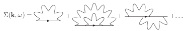
Figure 1: Diagrammatical expansion of the self-energy $\Sigma(\mathbf{k},\omega)$.

Of course this system can be solved trivially in the limit of $g=0$, in which case $G(\mathbf{k},\omega)=G_{0}(\mathbf{k},\omega)$ directly from Eq. (7). Also, in the limit of $t=0$ the free propagators become independent of momentum and the equivalent of the Lang-Firsov result is reproduced.goodvin However, for the general case of finite $g$ and $t$, a closed form solution cannot be obtained, even for the Holstein model.goodvin Approximations are therefore needed. We begin by describing the simplest MA⁽⁰⁾ version of a generalized MA approximation.

II.2 The MA⁽⁰⁾ Approximation

For the Holstein model, the MA⁽⁰⁾ approximation amounts to replacing all of the free electron propagators in the diagrammatical expansion of the self-energy by their momentum average over the Brillouin zone:

$$\bar{g}_{0}(\omega)=\frac{1}{N}\sum_{q}G_{0}(\mathbf{q},\omega),$$ (14)

which is equivalent to replacing all $G_{0}(\mathbf{k}-\mathbf{q}_{T},\omega-n\Omega)$ by $\bar{g}_{0}(\omega-n\Omega)$ in Eq. (13). The procedure is essentially the same for momentum-dependent electron-phonon couplings. We note that the first term from the $n=1$ case of Eq. (13) does not actually require any approximation (this is trivially true in the case in the Holstein model) because $f_{0}\equiv 1$ by definition, and its coefficient can be written explicitly as

$$\bar{\bar{g}}_{0}(\mathbf{k},\omega)=\frac{1}{N}\sum_{\mathbf{q}}|g_{\mathbf{q}}|^{2}G_{0}(\mathbf{k}-\mathbf{q},\omega).$$ (15)

By making the substitution $G_{0}(\mathbf{q},\omega-n\Omega)\to\bar{g}_{0}(\omega-n\Omega)$ everywhere else, we can rewrite Eqs. (12) and (13) in terms of the momentum averaged functions ${\cal F}_{n}(\mathbf{k},\omega)={1\over N^{n}}\sum_{\mathbf{q}_{1},\dots,\mathbf{q}_{n}}f_{n}(\mathbf{q}_{1},\ldots,\mathbf{q}_{n})$. This leads to simple recurrence relations linking each ${\cal F}_{n}$ to ${\cal F}_{n-1}$ and ${\cal F}_{n+1}$, and these can be solved in terms of continued fractions.goodvin ; berciu2 We find

$$\Sigma_{MA^{(0)}}(\mathbf{k},\omega)=\frac{\bar{\bar{g}}_{0}(\mathbf{k},\omega-\Omega)}{1-\bar{g}^{2}\bar{g}_{0}(\omega-\Omega)A_{2}(\omega)},$$ (16)

where we have defined the infinite continued fractions

$$A_{n}(\omega)= \frac{n\bar{g}_{0}(\omega-n\Omega)}{1-\bar{g}^{2}\bar{g}_{0}(\omega-n\Omega)A_{n+1}(\omega)}$$ (17)

$$= \cfrac{n\bar{g}_{0}(\omega-n\Omega)}{1-\cfrac{(n+1)\bar{g}^{2}\bar{g}_{0}(\omega-n\Omega)\bar{g}_{0}(\omega-(n+1)\Omega)}{1-\cdots}},$$

and the momentum averaged electron-phonon coupling:

$$\bar{g}^{2}=\frac{1}{N}\sum_{\mathbf{q}}|g_{\mathbf{q}}|^{2}.$$ (18)

It is trivial to check that this reduces to the Holstein result of Ref. goodvin, when $g_{\mathbf{q}}$ is independent of momentum.

Before we discuss how to systematically improve this result, we briefly review one explanation as to why this is a reasonable first step in obtaining an accurate approximation: in real space this approximation is equivalent to replacing, in all self-energy diagrams, all free propagators $G_{0}(i,j,\omega-n\Omega)\rightarrow\delta_{i,j}\bar{g}_{0}(\omega-n\Omega)$, where $i$ and $j$ index the electron sites.barisic ; berciu3 If the free propagators $G_{0}(i,j,\omega-n\Omega)$ are evaluated for energies well below the free electron continuum (and for a system with interactions the polaron ground state is below the free electron continuum), it is well known that the free propagator decreases exponentially with increasing distance $|i-j|$. Thus, the most important terms are those with $i=j$, i.e. precisely those included within MA⁽⁰⁾, explaining why the approximation should be reasonably accurate at low energies (spectral weight sum rules then insure that it is similarly accurate for all energies).

This also suggests a means to systematically improve the MA⁽⁰⁾ approximation. Since the propagators with the higher energy (the energy closer to the free-electron continuum) decrease exponentially with distance most slowly, the first improvement is to keep all propagators with energy $\omega-\Omega$ exactly. Higher order systematic improvements denoted by MA⁽ⁿ⁾ would amount to keeping all propagators with the argument $\omega-m\Omega$ exactly, for all $m\leq n$. In Ref. berciu2, we derived explicitly the Holstein MA self-energy for both $n=1$ and $n=2$. As shown and explained there, the $n=1$ order already insures the key improvement of properly predicting the polaron+one phonon continuum, which is usually absent at the $n=0$ level. The reason we went to $n=2$ for Holstein is that, given the simplicity of that model, only at the MA⁽²⁾ level did we find a momentum-dependent self-energy.

In contrast, for a model with a momentum-dependent coupling even the MA⁽⁰⁾ level gives explicit $\mathbf{k}$ dependence in the self-energy [see Eq. (16)], therefore in the next subsection we only consider the MA⁽¹⁾ generalization.

II.3 The MA⁽¹⁾ Approximation

The main drawback of the MA⁽⁰⁾ level of approximation is that it predicts an incorrect location for the electron+phonon continuum that must start at $E_{GS}+\Omega$. This problem is always “cured” at the MA⁽¹⁾ level because in real space MA⁽¹⁾ includes states with a phonon cloud near the electron and a single phonon arbitrarily far away, in other words precisely the type of states that give rise to the polaron+phonon continuum.berciu2 Mathematically, MA⁽¹⁾ amounts to keeping all propagators with the argument $\omega-\Omega$ in Eq. (13) exactly. Such terms only appear in the $n=1$ equation:

$$f_{1}^{(1)}(\mathbf{q}_{1})=G_{0}(\mathbf{k}-\mathbf{q}_{1},\omega-\Omega)\left[|g_{\mathbf{q}_{1}}|^{2}+\frac{1}{N}\sum_{\mathbf{q}_{2}}f_{2}^{(1)}(\mathbf{q}_{1},\mathbf{q}_{2})\right],$$ (19)

where we have distinguished the approximated $f_{n}$ terms with the superscript (1) to indicate the MA⁽¹⁾ level of approximation. For the remaining equations ($n\geq 2)$ we proceed as before, replacing $G_{0}(\mathbf{k}-\mathbf{q}_{T},\omega-n\Omega)$ with $g_{0}(\omega-n\Omega)$ everywhere in Eq. (13):

$$f_{n}^{(1)}(\mathbf{q}_{1},\ldots,\mathbf{q}_{n})=\bar{g}_{0}(\omega-n\Omega)\\ \times\left[\sum_{i=1}^{n}|g_{\mathbf{q}_{1}}|^{2}f_{n-1}^{(1)}(\ldots,\mathbf{q}_{i-1},\mathbf{q}_{i+1},\ldots)\right.\\ \left.+\frac{1}{N}\sum_{\mathbf{q}_{n+1}}f_{n+1}^{(1)}(\mathbf{q}_{1},\ldots,\mathbf{q}_{n+1})\right].$$ (20)

We wish to solve for $\Sigma_{MA^{(1)}}(\mathbf{k},\omega)=(1/N)\sum_{\mathbf{q}_{1}}f_{1}^{(1)}(\mathbf{q}_{1})$. The procedure is analogous to that of Ref. berciu2, . We obtain two sets of coupled recurrence relations, one for fully momentum averaged quantities ${\cal F}_{n}(\mathbf{k},\omega)={1\over N^{n}}\sum_{\mathbf{q}_{1},\dots,\mathbf{q}_{n}}f^{(1)}_{n}(\mathbf{q}_{1},\ldots,\mathbf{q}_{n})$ that already appeared at MA⁽⁰⁾ level, and one for partially averaged quantities $\bar{\cal F}_{n}(\mathbf{q_{1}},\mathbf{k},\omega)={1\over N^{n-1}}\sum_{\mathbf{q}_{2},\dots,\mathbf{q}_{n}}f^{(1)}_{n}(\mathbf{q}_{1},\ldots,\mathbf{q}_{n})$. Their solution follows the procedure detailed in Ref. berciu2, , and we simply state the result:

$$\Sigma_{MA^{(1)}}(\mathbf{k},\omega)=\frac{\bar{\bar{g}}_{0}(\mathbf{k},\tilde{\omega})}{1-\bar{\bar{g}}_{0}(\mathbf{k},\tilde{\omega})\left[A_{2}(\omega)-A_{1}(\omega-\Omega)\right]},$$ (21)

where $\tilde{\omega}=\omega-\Omega-\bar{g}^{2}A_{1}(\omega-\Omega)$. This expression is slightly more complicated than the expression for $\Sigma_{MA^{(0)}}(\mathbf{k},\omega)$ because it involves two continued fractions, but it is again trivial to compute numerically.

II.4 MA⁽⁰⁾ and MA⁽¹⁾ Results

To illustrate the accuracy of MA⁽⁰⁾ and MA⁽¹⁾ we will use the 1D breathing-mode Hamiltonian described by Eqs. (1) and (5) as an example, comparing our results to those found numerically using ED in Ref. lau, .

Before reporting these results we briefly discuss how the MA results are evaluated in practice. First, the numerical evaluation of the infinite continued fraction found in Eq. (16) requires that we truncate the fraction at some level $n$. For an error of order $\epsilon$ we require that at the $n^{\textrm{th}}$ level we have $\epsilon>ng^{2}\bar{g}_{0}(\omega-n\Omega)\bar{g}_{0}(\omega-(n+1)\Omega)$. Since $\bar{g}_{0}(\omega)\rightarrow 1/\omega$ when $|\omega|\to\infty$, for large enough $n$ we can approximate $\bar{g}_{0}(\omega-n\Omega)\approx\bar{g}_{0}(\omega-(n+1)\Omega)\approx-1/(n\Omega)$. It then follows that for an error of order $\epsilon$, we must have

$$n>\frac{1}{\epsilon}\frac{g^{2}}{\Omega^{2}}.$$ (22)

In practice we always check our results by doubling the value of the truncation value $n$ until the change in the self-energy is negligible. The result is that all MA error bars throughout this paper are smaller than the thickness of the lines/symbols used in the plots.

With our approximations for the Green’s function in hand, the ground-state properties are found by tracking the energy and weight of the lowest pole of the spectral weight, defined as

$$A(\mathbf{k},\omega)=-\frac{1}{\pi}\textrm{Im}\,\,G(\mathbf{k},\omega)=\sum_{\alpha}|\langle|\alpha|c_{\mathbf{k}}^{\dagger}|0\rangle|^{2}\delta(\omega-E_{\alpha}),$$ (23)

where a small but finite value of $\eta$ broadens the $\delta$ peaks into Lorentzians and enables us to detect them numerically (typically we take $\eta\sim 10^{-5}$). A detailed description on how we use the Green’s function to extract the energy spectrum and quasiparticle (qp) weights, as well as other quantities of interest such as effective masses, average number of phonons in the polaron cloud, etc., is presented in Ref. goodvin, . The explicit expressions for $\bar{g}_{0}(\omega)$ and $\bar{\bar{g}}_{0}(k,\omega)$ needed to compute the self-energies for the 1D breathing-mode Hamiltonian are given in Appendix A. As is customary, we define the dimensionless effective coupling $\lambda$ as the ratio between the lattice deformation energylau $-2g^{2}/\Omega$ and the free electron ground state energy $-2t$:

$$\lambda=\frac{g^{2}}{\Omega t}.$$ (24)

In Fig. 2 we plot the ground-state energy and qp weight as a function of the electron-phonon coupling strength, for a phonon energy $\Omega/t=0.5$.

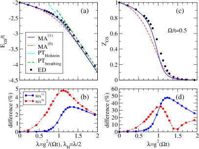
Figure 2: (Color online) (a) Ground state energy, (b) Percent difference from ED ground state energy results, (c) Ground state qp weight, and (d) Percent difference from ED qp weight results, as a function of the effective coupling $\lambda$, for $t=1,\Omega/t=0.5$. The perturbation theory resultslau for both the Holstein and breathing-mode models are shown, and the Holstein result is plotted as a function of $\lambda_{H}=\lambda/2$. The ED results are from Ref. lau, .

The MA⁽⁰⁾ (red dashed line) and MA⁽¹⁾ (solid blue line) results both show good agreement with the ED results (black circles). The ground state energies calculated with MA⁽⁰⁾ are within 5% error of the ED results, and the MA⁽¹⁾ results are better, coming within 3% error of the exact energies. They are exact for both $t=0$ and $\lambda=0$, as expected, and the crossover from the large to small polaron is captured to a high degree of accuracy. This accuracy is very encouraging, especially since these approximations are so trivial to evaluate. It is also worth pointing out that our work on the Holstein Hamiltonian shows that this accuracy improves in higher-dimensional models, and we believe this to be true here as well. Unfortunately, lack of detailed numerical results in higher dimensions prevents us from confirming this to be the case for models with momentum-dependent coupling.

Two more observations are apparent regarding these results: (i) The energies predicted by MA are lower in energy than the ED results, and (ii) the MA results approach the Lang-Firsov asymptotic limit very slowly.

The fact that the energies predicted are below the exact result indicates that the MA approximation is non-variational in the case of the breathing-mode model. This is somewhat surprising, since for the Holstein model it has been shown that MA⁽⁰⁾ is variationalbarisic ; berciu3 and that MA⁽¹⁾ is quasi-variational (in the latter case the Hamiltonian is modified slightly and the approximation is no longer truly variational, for details see Ref. berciu2, ). In any case, the energies found for the Holstein model using the semi-variational MA⁽¹⁾ and MA⁽²⁾ approximations were always higher than the exact numerical results.

The slow asymptotic convergence at large $\lambda$ is due to a different prefactor of the ${\cal O}(t^{2})$ perturbational correction. Instead of the correct breathing-mode resultlau

$$E_{B}(k)=-\frac{2g^{2}}{\Omega}-2t\cos(ka)e^{-3g^{2}/\Omega^{2}}\\ -\frac{\Omega t^{2}}{g^{2}}\left[\frac{1}{3}+\frac{e^{-2g^{2}/\Omega^{2}}}{2}\cos(2ka)\right],$$ (25)

we have produced the Holstein result from Ref. goodvin, with $g^{2}$ replaced with $\bar{g}^{2}=2g^{2}$ [see the two dashed lines labeled PT in Fig. 2(a)]:

$$E_{H}(k)=-\frac{2g^{2}}{\Omega}-2t\cos(ka)e^{-2g^{2}/\Omega^{2}}\\ -\frac{\Omega t^{2}}{g^{2}}\left[\frac{1}{2}+e^{-2g^{2}/\Omega^{2}}\cos(2ka)\right].$$ (26)

To understand the origin for both of these facts, we observe that at this level of approximations, almost all dependence on the el-ph coupling $g_{\mathbf{q}}$ is through its momentum-averaged value $\bar{g}^{2}=1/N\sum_{q}|g_{q}|^{2}$. For the 1D breathing-mode model, this average happens to be the same whether $g_{q}\propto i\sin{qa\over 2}$, as is the case here, or whether $g_{q}\propto\cos{qa\over 2}$ which would correspond to a coupling of the electron to the sum $x_{i-{1\over 2}}+x_{i+{1\over 2}}$ of O-site displacements. In other words, for this model, these simplest versions of the MA approximation register that a phonon cloud is formed at a certain O site, but not whether this leads to a leftwards or rightwards displacement of that site. In the strong coupling limit, one expects clouds to be formed only on the two O sites neighboring the Cu site that hosts the charge, and to point towards the charge. The effective hopping is related to the overlap of these clouds when the charge hops to a neighboring site. If the electron hops from $i$ to $i+1$, the phonon cloud at $i+{1\over 2}$ changes from $\exp{[-{g\over\Omega}b^{\dagger}_{i+{1\over 2}}]}|0\rangle$ to $\exp{[{g\over\Omega}b^{\dagger}_{i+{1\over 2}}]}|0\rangle$ and the overlap is small. In the MA approximations, it is precisely this information about left vs. right that is lost (equivalently, one can think of losing the information about relative phases between various contributions to the phonon cloud) and the overlap is unity – both cases have a cloud on the $i+{1\over 2}$ site. This explains the higher polaron mobility, hence the lower energy and slower convergence towards the exact asymptotic value for the MA approximations.

For the Holstein model, this problem does not appear because the el-ph coupling is local. We argue that this problem should also become less serious if the el-ph coupling is longer range, because in that case the relative sign of various displacements is not completely lost in the $\bar{g}^{2}=1/N\sum_{q}|g_{q}|^{2}$ average. Unfortunately, lack of numerical data for lattice models with longer-range el-ph coupling makes it difficult to support this statement. The only comparison we can offer is with the exact solution of a somewhat pathological, infinite-range coupling model called the HIC model of Ref. HIC, . As shown in Fig. 3, for this model both MA⁽⁰⁾ and MA⁽¹⁾ approximations give the correct asymptotic behavior – and this necessitates a correct description of the infinite-range phonon clouds that appear in this model.

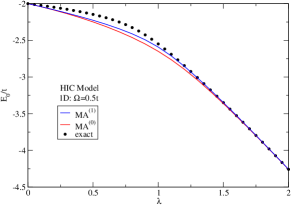
Figure 3: MA⁽⁰⁾ and MA⁽¹⁾ predictions of the ground-state energy of the HIC modelHIC as compared to its exact solution (black dots). For this model with infinite-range electron-phonon coupling, the approximations capture the correct asymptotic behavior.

To summarize, the MA approximations given by Eqs. (16) and (21) are very easy-to-use, and rather accurate for models with momentum-dependent electron-phonon coupling. Given its low dimension and short-range (but not local) el-ph interaction, one would expect the 1D breathing-mode model to be amongst the worst examples for the accuracy of this approximation. However, even here we obtain very decent agreement. As argued, we expect this to improve for higher dimensions and longer-range interactions. The only regime where accuracy is certain to worsen is when $\Omega/t$ becomes very small (this is a general problem of MA-like approximations, discussed at length in Ref. goodvin, ). Therefore, we believe that these approximations are useful for quick guides to relevant energies and other quantities of interest for problems of this type, obtained with minimal analytical and computational effort, yet still reasonably accurate.

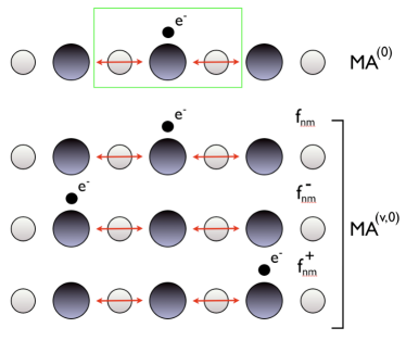
Figure 4: The generalized Green’s functions that appear in MA⁽⁰⁾ are sketched in the top picture. They have phonon clouds on two neighboring sites, with the electron on the central site. For the variational MA approximation, denoted MA^(v,0), we find again such Green’s functions, but also those with the electron to the immediate left or right of the phonon clouds. We name them $f_{nm}$ and $f^{\mp}_{nm}$, respectively.

III The variational Momentum Average Approximation

In this section, we attempt to remedy the problems pointed out in the previous section and by so doing, to obtain an improved MA approximation for the 1D breathing-mode Hamiltonian. The solution, which is presented in this section, can then be used as a template for any other $g_{\mathbf{q}}$ model. The main idea is to try to formulate an MA approximation which is variational in nature, as the original MA is for the Holstein Hamiltonian.berciu2 ; barisic

III.1 The MA^(v,0) Approximation

Given the good agreement found in the previous section, it is reasonable to use the MA⁽⁰⁾ solution as a guidance for what states are most relevant to include. Remember that this solution involved only the fully momentum-average quantities ${\cal F}_{n}({\mathbf{k}},\omega)={1\over N^{n}}\sum_{\mathbf{q}_{1},\dots,\mathbf{q}_{n}}f_{n}(\mathbf{k},\mathbf{q}_{1},\dots,\mathbf{q}_{n},\omega)$. Using the definition of Eqs. (9) and (6) and performing the sums over $q_{1},\dots q_{n}$ for our specific model with $g_{q}$ given by Eq. (5), we find immediately that ${\cal F}_{n}\propto\sum_{i}e^{ikR_{i}}\langle 0|c_{\mathbf{k}}\hat{G}(\omega)c_{i}^{\dagger}(b_{i-{1\over 2}}^{\dagger}-b_{i+{1\over 2}}^{\dagger})^{2}|0\rangle$. In other words, only states where there are phonons only on two neighboring sites contribute to it.

We use this as the criterion for our variational MA approximation. More specifically, when we use the Dyson equation to generate equations of motion, we only keep the terms which have phonons only on two neighboring sites, and discard any other contribution. Of course, these states have to have a total momentum $k$, or else the matrix element is zero. We find that 3 sets of generalized Green’s functions, sketched in Fig. 4, appear when we use this criterion, namely:

$$f_{n,m}=\frac{1}{\sqrt{N}G(k,\omega)}\sum_{i}e^{ikR_{i}}\langle 0|c_{k}\hat{G}(\omega)c_{i}^{\dagger}b_{i-\frac{1}{2}}^{\dagger m}b_{i+\frac{1}{2}}^{\dagger n-m}|0\rangle$$ (27)

and

$$f^{\pm}_{n,m}=\frac{1}{\sqrt{N}G(k,\omega)}\sum_{i}e^{ikR_{i}}\langle 0|c_{k}\hat{G}(\omega)c_{i\pm 1}^{\dagger}b_{i-\frac{1}{2}}^{\dagger m}b_{i+\frac{1}{2}}^{\dagger n-m}|0\rangle.$$ (28)

Note: as before, we again we do not write explicitly the $k$ and $\omega$ dependence.

It is straightforward to show that in this notation we can write Eq. (10) as

$$G(k,\omega)=G_{0}(k,\omega)[1+g(f_{1,0}-f_{1,1})G(k,\omega)],$$ (29)

and therefore

$$\Sigma_{MA^{(v,0)}}(k,\omega)=g(f_{1,0}-f_{1,1}).$$ (30)

The equations of motion consistent with the variational restriction are straightforward to find:

$$f_{n,0}=e_{0}\left[nf_{n-1,0}+f_{n+1,0}-f_{n+1,1}\right]-e_{2}e^{-ika}f^{+}_{n+1,n}\\ -e_{1}\left[ne^{-ika}f_{n-1,n-1}-e^{-ika}f_{n+1,n}+e^{-ika}f_{n+1,n+1}-f^{-}_{n+1,1}\right]$$ (31)

For any $1\leq m\leq n-1$,

$$f_{n,m}=e_{0}\left[(n-m)f_{n-1,m}-mf_{n-1,m-1}+f_{n+1,m}-f_{n+1,m+1}\right]\\ -e_{1}\left[(n-m)f^{+}_{n-1,m}-mf^{-}_{n-1,m-1}+f^{+}_{n+1,m}-f^{-}_{n+1,m+1}\right],$$ (32)

and

$$f_{n,n}=-e_{0}\left[nf_{n-1,n-1}+f_{n+1,n+1}-f_{n+1,n}\right]+e_{2}e^{ika}f^{-}_{n+1,1}\\ +e_{1}\left[ne^{ika}f_{n-1,0}-e^{ika}f_{n+1,1}+e^{ika}f_{n+1,0}-f^{+}_{n+1,n}\right].$$ (33)

Similarly, for any $1\leq m\leq n-1$,

$$f^{\pm}_{n,m}=e_{1}\left[(n-m)f_{n-1,m}-mf_{n-1,m-1}+f_{n+1,m}-f_{n+1,m+1}\right]\\ -\left\{\begin{array}[]{c}e_{0}\\ e_{2}\end{array}\right\}\left[(n-m)f^{+}_{n-1,m}+f^{+}_{n+1,m}\right]+\left\{\begin{array}[]{c}e_{2}\\ e_{0}\end{array}\right\}\left[mf^{-}_{n-1,m-1}+f^{-}_{n+1,m+1}\right]$$ (34)

and

$$f^{-}_{n,0}=e_{1}\left[nf_{n-1,0}+f_{n+1,0}-f_{n+1,1}\right]+e_{0}f^{-}_{n+1,1}-e_{3}e^{-ika}f^{+}_{n+1,n}\\ -e_{2}\left[ne^{-ika}f_{n-1,n-1}+e^{-ika}f_{n+1,n+1}-e^{-ika}f_{n+1,n}\right]$$ (35)

$$f^{+}_{n,n}=-e_{1}\left[nf_{n-1,n-1}+f_{n+1,n+1}-f_{n+1,n}\right]-e_{0}f^{+}_{n+1,n}+e_{3}e^{ika}f^{-}_{n+1,1}\\ +e_{2}\left[ne^{ika}f_{n-1,0}+e^{ika}f_{n+1,0}-e^{ika}f_{n+1,1}\right]$$ (36)

where we use the shorthand notation $e_{j}=g\bar{g}_{j}(\omega-n\Omega)$, and $\bar{g}_{j}(\omega)$ are real-space Green’s functions, defined as

$$\bar{g}_{j}(\omega)=\frac{1}{N}\sum_{q}e^{\pm iq(ja)}G_{0}(q,\omega)=G_{0}(j,0,\omega).$$ (37)

The “$\pm$” sign in the exponent of Eq. (37) is irrelevant because $G_{0}(q,\omega)$ is even with respect to $q$. The explicit expressions for these and other momentum averaged functions of the free electron propagator are given in Appendix A for a tight-binding dispersion. Note that $f^{-}_{n,n}=e^{ika}f_{n,0}$ and $f^{+}_{n,0}=e^{-ika}f_{n,0}$, which is why we do not need to keep them as independent variables.

Equations (31)-(36) can now be cast in the form $\mathbf{v}_{n}=\mathrm{A}_{n}\mathbf{v}_{n-1}+\mathrm{B}_{n}\mathbf{v}_{n+1}$, where

$$\mathbf{v}_{n}=\left(f_{n,0},\ldots,f_{n,n},f^{-}_{n,0},\ldots,f^{-}_{n,n-1},f^{+}_{n,1},\ldots,f^{+}_{n,n}\right)^{T}$$ (38)

collects all generalized Green’s functions with a total of $n$ phonons, and the matrices $\mathrm{A}_{n},\mathrm{B}_{n}$ are straightforward to obtain from the equations above. The solution of this set of recursive equations can then be written as an infinite continued fraction involving products of matrices:

$$\mathbf{v}_{n}=\mathrm{Q}_{n}\mathbf{v}_{n-1}=\cfrac{1}{1-\mathrm{B}_{n}\mathrm{Q}_{n+1}}\mathrm{A}_{n}\mathbf{v}_{n-1}.$$ (39)

Although this is a continued fraction of matrices of increasing size, it is still numerically trivial to evaluate. The dimensions of $\mathrm{A}_{n}$ and $\mathrm{B}_{n}$ are $(3n+1)\times(3n-2)$ and $(3n+1)\times(3n+4)$, respectively, and we determine the truncation level of the continued fraction using the same criteria as discussed in the previous section for the MA⁽⁰⁾ approximation. In addition, the $\mathrm{A}_{n}$ and $\mathrm{B}_{n}$ matrices are very sparse, which makes multiplication by them very efficient. Finally, since $v_{0}\equiv 1$ by definition, it is straightforward to calculate $\Sigma_{MA^{(v,0)}}(k,\omega)$ from Eq. (30) once $v_{1}=(f_{1,0},f_{1,1},f^{-}_{1,0},f^{+}_{1,1})^{T}=\mathrm{Q}_{1}$ is evaluated from Eq. (39).

III.2 MA^(v,1) approximation

We can also systematically improve the variational MA approximation to reproduce the electron+phonon continuum. It is obvious that this will not be predicted by MA^(v,0), since no phonons are allowed to appear far from the main polaronic cloud.

We follow the same approach as before: at the MA^(v,1) level we keep all equations involving free electron propagators with $\omega-\Omega$ exactly. In order to work in the enlarged variational space described by Eqs. (27) and (28) we need to define the following generalized Green’s functions (these are analogous to the partial momentum averages $\bar{{\cal F}}(\mathbf{q}_{1},\mathbf{k},\omega)$):

$$\bar{f}_{n,m}(q_{1})=\frac{g_{q_{1}}}{\sqrt{N}G(k,\omega)}\sum_{i}e^{i(k-q_{1})R_{i}}\\ \times\langle 0|c_{k}\hat{G}(\omega)c_{i}^{\dagger}b_{q_{1}}^{\dagger}b_{i-\frac{1}{2}}^{\dagger m}b_{i+\frac{1}{2}}^{\dagger(n-1)-m}|0\rangle$$ (40)

and

$$\bar{f}^{\pm}_{n,m}(q_{1})=\frac{g_{q_{1}}}{\sqrt{N}G(k,\omega)}\sum_{i}e^{i(k-q_{1})R_{i}}\\ \times\langle 0|c_{k}\hat{G}(\omega)c_{i\pm 1}^{\dagger}b_{q_{1}}^{\dagger}b_{i-\frac{1}{2}}^{\dagger m}b_{i+\frac{1}{2}}^{\dagger(n-1)-m}|0\rangle.$$ (41)

These Green’s functions explicitly contain states with one phonon delocalized away from the main polaronic cloud, i.e. precisely the type of states required to reproduce the polaron+phonon continuum. In this notation Eq. (19) can be written as

$$f_{1}(q_{1})=G_{0}(k-q_{1},\omega-\Omega)\left[|g_{q_{1}}|^{2}+g(\bar{f}_{2,0}(q_{1})-\bar{f}_{2,1}(q_{1}))\right],$$ (42)

which is an exact equation involving no approximations, as in the MA⁽¹⁾ case.

We can immediately use the MA^(v,0) result to solve Eq. (20), but only up to the $n=2$ level: $\mathbf{v}_{2}=\mathrm{Q}_{2}\mathbf{v}_{1}$. To solve the $n=1$ equation exactly we will need to construct a set of recurrence relations involving Eqs. (40) and (41) using Dyson’s identity. The resulting equations take a form similar to Eqs. (31)-(36) if we define

$$\delta f_{n,m}(q_{1})=\bar{f}_{n,m}(q_{1})-g(1-e^{iq_{1}})f_{n,m}\\ +g(1-e^{-iq_{1}})f_{n,m+1},$$ (43)

$$\delta f_{n,0}(q_{1})=\bar{f}_{n,0}(q_{1})-g(1-e^{iq_{1}})f_{n,0}\\ +g(1-e^{-iq_{1}})f_{n,1}-ge^{-i(k-q_{1})}(1-e^{iq_{1}})f^{-}_{n,n-1},$$ (44)

$$\delta f_{n,n-1}(q_{1})=\bar{f}_{n,n-1}(q_{1})-g(1-e^{iq_{1}})f_{n,n-1}\\ +g(1-e^{-iq_{1}})f_{n,n}+ge^{i(k-q_{1})}(1-e^{-iq_{1}})f^{+}_{n,1},$$ (45)

for $n>1$, and

$$\delta f_{1,0}(q_{1})=\bar{f}_{1,0}(q_{1})-g(1-e^{iq_{1}})f^{(1)}_{1,0}+g(1-e^{-iq_{1}})f^{(1)}_{1,1}\\ -ge^{-i(k-q_{1})}(1-e^{iq_{1}})f^{-(1)}_{1,0}+ge^{i(k-q_{1})}(1-e^{-iq_{1}})f^{+(1)}_{1,1}.$$ (46)

We have again added the superscript $(1)$ to distinguish $f^{(1)}_{1,0},f^{(1)}_{1,1},f^{-(1)}_{1,0},f^{+(1)}_{1,1}$ from the MA^(v,0) expressions. With these definitions, the recurrence relations for the $\delta f_{n,m}$ functions have precisely the same form as Eqs. (31)-(36) with $n\to n-1$ and $\omega\to\omega-\Omega$. As before, we write this set of equations in the form $\delta\mathbf{v}_{n}=\mathrm{A}^{\prime}_{n}\delta\mathbf{v}_{n-1}+\mathrm{B}^{\prime}_{n}\delta\mathbf{v}_{n+1}$, where

$$\delta\mathbf{v}_{n}=\left(\delta f_{n,0},\ldots,\delta f_{n,n-1},\right.\\ \left.\delta f^{-}_{n,0},\ldots,\delta f^{-}_{n,n-2},\delta f^{+}_{n,1},\ldots,\delta f^{+}_{n,n-1}\right)^{T},$$ (47)

and the solution can again be written in terms of an infinite continued fraction of matrices:

$$\delta\mathbf{v}_{n}=\mathrm{R}_{n}\delta\mathbf{v}_{n-1}=\cfrac{1}{1-\mathrm{B}^{\prime}_{n}\cfrac{1}{1-\cdots}\mathrm{A}^{\prime}_{n+1}}\mathrm{A}^{\prime}_{n}\delta\mathbf{v}_{n-1},$$ (48)

where $\mathrm{A}^{\prime}_{n}(\omega)=\mathrm{A}_{n-1}(\omega-\Omega)$ and $\mathrm{B}^{\prime}_{n}(\omega)=\mathrm{B}_{n-1}(\omega-\Omega)$.

To finish the calculation we will require explicit expressions for $f^{(1)}_{1,0},f^{(1)}_{1,1},f^{-(1)}_{1,0},$ and $f^{+(1)}_{1,1}$. Using the definitions in Eqs. (27), (28), (40), and (41) it is straightforward to show that

$$f^{(1)}_{1,0}=\frac{1}{N}\sum_{q_{1}}G_{0}(k-q_{1},\omega-\Omega)\frac{1}{1-e^{iq_{1}}}\\ \times\left[\bar{f}_{2,0}(q_{1})-\bar{f}_{2,1}(q_{1})\right]+e_{0}-e_{1}e^{-ika},$$ (49)

$$f^{(1)}_{1,1}=-\frac{1}{N}\sum_{q_{1}}G_{0}(k-q_{1},\omega-\Omega)\frac{1}{1-e^{-iq_{1}}}\\ \times\left[\bar{f}_{2,0}(q_{1})-\bar{f}_{2,1}(q_{1})\right]-e_{0}+e_{1}e^{ika},$$ (50)

$$f^{-(1)}_{1,0}=\frac{1}{N}\sum_{q_{1}}e^{i(k-q_{1})}G_{0}(k-q_{1},\omega-\Omega)\frac{1}{1-e^{iq_{1}}}\\ \times\left[\bar{f}_{2,0}(q_{1})-\bar{f}_{2,1}(q_{1})\right]+e_{1}-e_{2}e^{-ika},$$ (51)

and

$$f^{+(1)}_{1,1}=-\frac{1}{N}\sum_{q_{1}}e^{-i(k-q_{1})}G_{0}(k-q_{1},\omega-\Omega)\frac{1}{1-e^{-iq_{1}}}\\ \times\left[\bar{f}_{2,0}(q_{1})-\bar{f}_{2,1}(q_{1})\right]-e_{1}+e_{2}e^{ika}.$$ (52)

To combine all of these results and obtain a system of four equations in the four unknowns $f^{(1)}_{1,0},f^{(1)}_{1,1},f^{-(1)}_{1,0},f^{+(1)}_{1,1}$, we need to rewrite $\bar{f}_{2,0}(q_{1})-\bar{f}_{2,1}(q_{1})$ in terms of these four quantities. Using the definitions in Eqs. (44)-(46), $\mathbf{v}_{2}=\mathrm{Q}_{2}\mathbf{v}_{1}$, and $\delta\mathbf{v}_{2}=\mathrm{R}_{1}\delta\mathbf{v}_{1}$, we find that

$$\bar{f}_{2,0}(q_{1})-\bar{f}_{2,1}(q_{1})=G_{0}^{-1}(k-q,\omega-\Omega)G_{0}(k-q,\tilde{\tilde{\omega}})\left\{(R_{00}-R_{10})\left[G_{0}(k-q_{1},\omega-\Omega)|g_{q_{1}}|^{2}\right.\right.\\ \left.\left.-g(1-e^{iq_{1}})f^{(1)}_{1,0}+g(1-e^{-iq_{1}})f^{(1)}_{1,1}-ge^{-i(k-q_{1})}(1-e^{iq_{1}})f^{-(1)}_{1,0}+ge^{i(k-q_{1})}(1-e^{-iq_{1}})f^{+(1)}_{1,1})\right]\right.\\ \left.+g(1-e^{iq_{1}})\mathrm{Q}_{2}\mathbf{v}_{1}|_{0}-2g\left[1-\cos(q_{1})\right]\mathrm{Q}_{2}\mathbf{v}_{1}|_{1}+g(1-e^{-iq_{1}})\mathrm{Q}_{2}\mathbf{v}_{1}|_{2}\right.\\ \left.+ge^{-i(k-q_{1})}(1-e^{iq_{1}})\mathrm{Q}_{2}\mathbf{v}_{1}|_{4}+ge^{i(k-q_{1})}(1-e^{-iq_{1}})\mathrm{Q}_{2}\mathbf{v}_{1}|_{5}\right\},$$ (53)

where $\tilde{\tilde{\omega}}=\omega-\Omega-g(R_{00}-R_{10})$. In this notation $R_{ij}$ are the matrix elements of $\rm{R}_{1}$ and $\mathrm{Q}_{2}\mathbf{v}_{1}|_{i}$ is the $i^{th}$ element of the product between the matrix $\rm{Q}_{2}$ and the vector $\mathbf{v}_{1}$, i.e., $\mathrm{Q}_{2}\mathbf{v}_{1}|_{i}=Q_{i0}f^{(1)}_{1,0}+Q_{i1}f^{(1)}_{1,1}+Q_{i2}f^{-(1)}_{1,0}+Q_{i3}f^{+(1)}_{1,1}$, where $Q_{ij}$ are the matrix elements of $\mathrm{Q}_{2}$. Inserting Eq. (53) into Eqs. (49)-(52), and performing the required sums over momentum, we obtain the desired four equations in four unknowns. The explicit expressions for the momentum averages that appear in these expressions are given in Appendix A. Once this system has been solved we can easily compute the self-energy as

$$\Sigma_{MA^{(v,1)}}(k,\omega)=g(f^{(1)}_{1,0}-f^{(1)}_{1,1}).$$ (54)

Again the MA^(v,1) expression is slightly more involved than the zeroth order approximation because we need to evaluate two continued fractions, but it is still numerically trivial to evaluate.

IV Results

We present results for the 1D breathing-mode Hamiltonian using the variational MA approximation. Comparisons are made to ED datalau where possible.

IV.1 Ground State Properties

In Fig. 5 we plot both the ground state energy and qp weight as a function of the electron-phonon coupling strength, using the variational MA approximation.

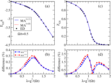
Figure 5: (Color online) (a) Ground state energy, (b) Percent difference from ED ground state energy results, (c) Ground state qp weight, and (d) Percent difference from ED qp weight results, as a function of the effective coupling $\lambda$, for $t=1,\Omega/t=0.5$. The ED results are from Ref. lau, .

The variational MA results show a clear improvement over the MA results shown in Fig. 2, and the agreement with the numerical data is excellent. The approximate and exact numerical data results are indistinguishable when plotted over the full parameter range of Fig. 5(a). To gain a closer look at the success of our approximation we plot the relative error between the MA results and the ED results in Fig. 5(b). Indeed the approximation is giving extremely close agreement with the numerical results, with less than 0.3% relative error for both MA^(v,0) and MA^(v,1). The largest errors occur at intermediate couplings, as expected because the MA approximation is exact in both the zero coupling and zero bandwidth limits. We also show a comparison of the quasiparticle weight calculated using variational MA with the ED result in Fig. 5(c). Again, when plotted over the full parameter range, the results are nearly indistinguishable. A look at the percent difference indicates that the relative error is less than 2.5%. This is a truly remarkable fact considering that the qp weight contains information on the nature of the eigenstates, something that is rarely obtained accurately when using approximate methods.

It is clear from Fig. 5 that the variational MA approximation cures all of the shortcomings of the simple MA generalization discussed in Sec. II.4. A comparison of the variational MA and ED results shows that the MA energies are slightly higher than the exact numerical results, as expected from a variational method, and that the asymptotic behavior predicted from both the perturbational theory and ED result is reproduced. These successes were expected because the variational MA approximation was designed precisely to remedy these problems, but it is still very encouraging to see that the physical picture described and used to motivate the variational MA approximation in Sec. III was indeed correct.

In Fig. 6(a) we plot the average number of phonons in the cloud, $N_{ph}$, as calculated from the Hellmann-Feynman theorem.goodvin Since there is no numerical data available for this quantity we compare our findings to the standard Rayleigh-Schrödinger (RS) perturbation theory at small couplings, and to the strong-coupling perturbation theory for larger couplings. The approximation reproduces both asymptotic limits to a high degree of accuracy, as should be expected based on the success of the ground state energies and qp weights shown in Fig. 5. Since we are unaware of any explicit expression for the RS energy for the breathing-mode Hamiltonian in the literature, we state the result here. By evaluating the standard expression for the first order correction

$$E_{\mathbf{k}}^{(1)}=-\frac{1}{N}\sum_{\mathbf{q}}\frac{g_{\mathbf{q}}^{2}}{\varepsilon_{\mathbf{k}-\mathbf{q}}+\Omega-\varepsilon_{\mathbf{k}}},$$ (55)

one can easily show that

$$E_{k}^{(1)}=-2g^{2}\bar{g}_{0}(\Omega-\varepsilon_{k})-\frac{g^{2}}{t}\cos k\left[1-(\Omega-\varepsilon_{k})\bar{g}_{0}(\Omega-\varepsilon_{k})\right]$$ (56)

for the 1D breathing-mode Hamiltonian.

In Fig. 6 we also plot the effective mass as a function of the coupling strength.

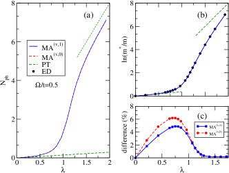
Figure 6: (Color online) (a) Average number of phonons and (b) effective mass, (c) Percent difference from ED effective mass results, as a function of the effective coupling $\lambda$, for $t=1,\Omega/t=0.5$. The ED results are from Ref. lau, .

Again the agreement with the numerical data is excellent, as confirmed by the relative errors shown in Fig. 6(c).

IV.2 The Polaron Band

With our analytical expression for the self-energy we can also calculate momentum-dependent results. In Fig. 7(a) we plot the lowest energy state for momenta $0\leq k\leq\pi$ and compare our results to the available numerical data.

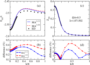
Figure 7: (Color online) (a) Polaron dispersion $E_{k}$, (b) Percent difference from ED ground state energy results, (c) quasiparticle weight $Z_{k}$, and (d) Percent difference from ED qp weight results. Results are shown for $t=1,\Omega/t=0.5$, and $\lambda=1.071502$. The ED results are from Ref. lau, .

We again find that the variational MA approximation is highly accurate. Because the polaron dispersion is relatively flat for the intermediate coupling strength of $\lambda=1.071502$ shown here, the energy range of the plot is quite narrow and we can clearly discern the difference between the approximate and numerical results. However, by looking at the relative error in Fig. 7(b), we demonstrate that the accuracy of the variational MA result is again very good, coming well within 0.5% relative error of the numerical result, showing that the variational MA approximation is accurate for all momenta $k$. The reason for the non-monotonic polaron dispersion has been discussed at length in Ref. lau, , and is due to a larger effective 2nd nearest neighbor hopping than the effective nearest neighbor hopping of the polaron – this is a direct consequence of the structure of the polaronic cloud. In Figs. 7(c) and 7(d) we plot the qp weight and its relative error as a function of momenta. We again find good agreement. As explaned, the agreement is expected to improve for both smaller and larger $\lambda$ values, where our approximations become asymptotically exact.

IV.3 Higher Energy Properties

Lastly, we consider the high energy properties of the 1D breathing-mode Hamiltonian using MA^(v,0) and MA^(v,1). In Fig. 8 we compare our predicted spectral weights to available numerical data.

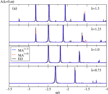
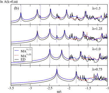
Figure 8: (Color online) (a) $A(k=0,\omega)$ vs. $\omega$ and (b) $\ln A(k=0,\omega)$ for $t=1,\Omega=0.5,\eta=0.004$, and $\lambda=0.75,1.0,1.25,1.5$; The vertical blue dashed lines denote $E_{gs}$ and $E_{gs}+\Omega$ using MA^(v,1). The ED results are from Ref. lau, .

When plotted on a linear axis, the results are essentially indistinguishable, especially for MA^(v,1). To gain a better view we display the same plots on a logarithmic scale in Fig. 8(b). There are a few interesting features to note. At the MA⁽⁰⁾ level (red dashed line) the majority of the spectral weight is found to be in the correct location, however, the electron+phonon continuum is completely absent for the parameters shown, as expected. At the MA^(v,1) level the continuum is reproduced in the expected location, in very good agreement with the ED prediction. Furthermore, the finite size effects responsible for the sharp peaks in the continuum of the ED result are absent from the MA^(v,1) data. As a guide illustrating the correct location for the polaron+phonon continuum we have added the vertical blue dashed lines to denote $E_{gs}$ and $E_{gs}+\Omega$ for the MA^(v,1) ground state energy. The lower edge is located correctly, however especially for smaller $\lambda$, MA predicts a somewhat wider continuum than ED. Given the very limited availability of numerical results of this type, we do not know if this discrepancy is due to truncation approximations in the ED solution, or is due to inaccuracies of the MA approximations.

In Fig. 9 we plot the spectral weight for a fixed coupling strength and vary the momentum $k$.

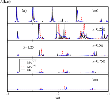
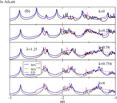
Figure 9: (Color online) (a) $A(k,\omega)$ and (b) $\ln A(k,\omega)$ vs. $\omega$ for $k/\pi=0,0.25,0.5,0.75,1$, $t=1,\Omega=0.5,\lambda=1.25,\eta=0.004$; The ED results are from Ref. lau, .

Again on the linear scale the results are very encouraging. The MA result, particularly MA^(v,1) predicts the correct location for the spectral weight over the entire energy range. However, a logarithmic scale plot does reveal a notable shortcoming of the approximation. For $k=0$ the agreement with the numerical data is excellent and the continuum is located at the expected $E_{gs}+\Omega$. For $k=0.25\pi$ and $k=0.5\pi$ the agreement is still good, but as we begin to approach the band edge we see a significant deviation of the MA result from the ED result, with the MA continuum coming to much too low energies. This feature has extremely little spectral weight (see Fig. 9(a)) and is extremely unlikely to be detectable in any experimental realization, however it is in stark disagreement with the expected result confirmed by the ED data. We do not currently understand this failure at higher $k$ values.

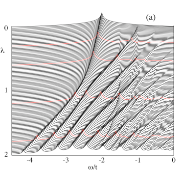
Figure 10: (Color online) Spectral weight $A(0,\omega)$ vs. $\omega$ in 1D using (a) MA^(v,0) and (b) MA^(v,1). The results are shown for $t=1,\Omega=0.5,\eta=0.01$, and $\lambda$ varying from 0 to 2. Curves corresponding to $\lambda=0.3,0.6,1.2$ and $1.8$ are highlighted in red.

Finally, in Fig. 10 we show more detailed plots of the evolution of the spectral weight for $k=0$ from zero coupling to large coupling, for a full range of energies. The two panels compare the MA^(v,0) (a) and MA^(v,1) (b) solutions. The one obvious difference is the location of the polaron+phonon continuum, which is incorectly located around $-2t$ for MA^(v,0), whereas it always starts at $\Omega$ above $E_{gs}$ for MA^(v,1). Aside from this feature with rather little weight, all the features which contribute significantly to the spectral weight are in good agreement.

Plots of this nature would require extensive numerical computational time if one tried to generate them using “exact” computational methods. For example, achieving convergence for the ED results at larger $\lambda$ required inclusion of billions of states, in some cases, in the truncated Hilbert space. Diagonalizing such large (even though sparse) matrices is not a trivial task. By comparison, because we have an analytical expression for the self-energy, these detailed MA plots covering many energies and couplings take just seconds, at most minutes, to generate. In fact, MA is much faster even than SCBA, which for this model requires many numerical integrals over the Brillouin zone (and is of questionable use for medium and large couplings).

V Summary and Conclusions

In summary, we have presented a way to generalize the momentum average approximation to more general electron-phonon coupling models with momentum-dependent couplings. The approximation still sums all of the self-energy diagrams, albeit with each diagram approximated in such a way that the full sum can be performed, and it is exact in both the zero coupling and zero bandwidth limits. As in the application of MA to the Holstein model, the approximation is analytical and easy-to-use, and gives highly accurate results over the entire parameter space. In this paper we have actually presented two different generalizations of MA, a straightforward generalization that can easily be applied to any model with a momentum-dependent coupling with minimal effort, and a more specific (and extremely accurate) generalization that takes the details of a given model into account and enlarges the variational subspace accordingly. We have used the 1D breathing-mode Hamiltonian as an example to gauge the accuracy of both of these MA generalizations. While the straightforward extension of MA gave fairly accurate results, it was non-variational and it approached the zero-bandwidth asymptotic limit very slowly. The variational MA approximation remedied both of these problems and produced extremely accurate results, coming well within 0.3% error of the available numerical results for the ground state energies of the breathing-mode polaron. We also showed that MA can be systematically improved in both cases, leading to higher accuracy and the correct location for the electron+phonon continuum.

The successful generalization of MA to this much broader class of models in very encouraging. Numerical studies of models as complicated as even the 1D breathing-mode Hamiltonian are very intensive, and the MA approximation provides a quick and easy-to-use way to gain an understanding of these more realistic models without having to do a detailed numerical analysis from the start. We hope that this tool will be extremely useful for probing more realistic and experimental realizations of interesting physical systems. The range of applicability of the MA approximation has been growing steadily. As mentioned previously, it has been successfully applied to systems with multiple phonon modes,covaci and multiple free-electron bands.covaci2 Other obvious and very useful generalizations of this approximation would be to apply it to finite particle densities and/or finite temperatures, and possibly to an even broader class of Hamiltonians involving electron-electron interactions.

Appendix A Momentum Averages

In this section we derive the various momentum averages required to evaluate the self-energy expressions derived in this work. We require the following weighted momentum averages of the free electron propagator for a 1D tight-binding dispersion:

$$\bar{g}_{j}(\omega)\equiv\frac{1}{N}\sum_{q}e^{\pm ik(ja)}G_{0}(q,\omega).$$ (57)

It is straightforward to show that

$$\bar{g}_{0}(\omega)=\frac{\textrm{sgn}(\omega+i\eta)}{\sqrt{(\omega+i\eta)^{2}-4t^{2}}},$$ (58)

$$\bar{g}_{1}(\omega)=\frac{1}{2t}\left[1-(\omega+i\eta)\bar{g}_{0}(\omega)\right],$$ (59)

$$\bar{g}_{2}(\omega)=-\bar{g}_{0}(\omega)-\frac{\omega+i\eta}{t}\bar{g}_{1}(\omega),$$ (60)

and

$$\bar{g}_{3}(\omega)=\frac{1}{t}-\left[3-\frac{(\omega+i\eta)^{2}}{t^{2}}\right]\bar{g}_{1}(\omega).$$ (61)

For the MA⁽⁰⁾ and MA⁽¹⁾ self-energy expressions we also require $\bar{\bar{g}}_{0}(\mathbf{k},\omega)$, as defined in Eq. (15). For the 1D breathing-mode model one can show that

$$\bar{\bar{g}}_{0}(k,\omega)=2g^{2}\bar{g}_{0}(\omega)-\frac{g^{2}\cos k}{t}\left[1-(\omega+i\eta)\bar{g}_{0}(\omega)\right].$$ (62)

In the MA^(v,1) calculation we require the momentum average of Eq. (53). For the 1D breathing-mode Hamiltonian (i.e. $g_{q}=-2ig\sin(q/2)$ and $\varepsilon_{k}=-2t\cos(k)$) we require the following momentum averages:

$$\frac{1}{N}\sum_{q}G_{0}(k-q,\omega)\frac{e^{\pm ni(k-q)}(1-e^{\mp iq})}{1-e^{\pm iq}}=-e^{\mp ik}\bar{g}_{n+1}(\omega),$$ (63)

$$\frac{1}{N}\sum_{q}G_{0}(k-q,\tilde{\omega})G_{0}(k-q,\omega)\frac{e^{\pm ni(k-q)}|g_{q}|^{2}}{1-e^{\pm iq}}\\ =\frac{g^{2}}{\omega-\tilde{\omega}}\left\{\bar{g}_{n}(\tilde{\omega})-\bar{g}_{n}(\omega)-e^{\mp ik}\left[\bar{g}_{n+1}(\tilde{\omega})-\bar{g}_{n+1}(\omega)\right]\right\},$$ (64)

and

$$\frac{1}{N}\sum_{q}G_{0}(k-q,\omega)\frac{e^{\pm ni(k-q)}(1-\cos q)}{1-e^{\pm iq}}\\ =\frac{1}{2}\left[\bar{g}_{n}(\omega)-e^{\mp ik}\bar{g}_{n+1}(\omega)\right].$$ (65)

References

- (1) M. Hengsberger, D. Purdie, P. Segovia, M. Garnier, and Y. Baer, Phys. Rev. Lett. 83, 592 (1999).
- (2) O. Gunnarsson, Rev. Mod. Phys. 69, 575 (1997), and references therein.
- (3) W. P. Su, J. R. Schrieffer, and A. J. Heeger, Phys. Rev. Lett. 42, 1698 (1979).
- (4) M. B. Salamon and M. Jaime, Rev. Mod. Phys. 73, 583 (2001).
- (5) F. Mila, Phys. Rev. B 52, 4788 (1995), and references therein.
- (6) A. La Magna and R. Pucci, Eur. Phys. J. B 4, 421 (1998).
- (7) A. Lanzara, P. V. Bogdanov, X. J. Zhou, S. A. Kellar, D. L. Feng, E. D. Lu, T. Yoshida, H. Eisaki, A. Fujimori, K. Kishio, J.-I. Shimoyama, T. Noda, S. Uchida, Z. Hussain and Z.-X. Shen, Nature 412, 510 (2001).
- (8) K. M. Shen, F. Ronning, D. H. Lu, W. S. Lee, N. J. C. Ingle, W. Meevasana, F. Baumberger, A. Damascelli, N. P. Armitage, L. L. Miller, Y. Kohsaka, M. Azuma, M. Takano, H. Takagi, and Z.-X. Shen, Phys. Rev. Lett. 93, 267002 (2004).
- (9) A. S. Mishchenko and N. Nagaosa, Phys. Rev. Lett. 93, 036402 (2004).
- (10) T. Cuk, D.H. Lu, X.J. Zhou, Z.-X. Zhen, T.P. Devereaux, and N. Nagaosa, PHys. Status Solidi B 242, 1 (2005).
- (11) M. Berciu, Phys. Rev. Lett. 97, 036402 (2006).
- (12) G. L. Goodvin, M. Berciu and G.A. Sawatzky, Phys. Rev. B 74, 245104 (2006).
- (13) M. Berciu, Phys. Rev. Lett. 98, 209702 (2007).
- (14) M. Berciu and G.L. Goodvin, Phys. Rev. B 76, 165109 (2007).
- (15) L. Covaci and M. Berciu, Europhys. Lett. 80, 67001 (2007).
- (16) L. Covaci and M. Berciu, Phys. Rev. Lett. 100, 256405 (2008).
- (17) B. Lau, M. Berciu and G. A. Sawatzky, Phys. Rev. B 76, 174305 (2007).
- (18) S.I. Pekar, E.I. Rashba, and V.I. Sheka, Zh Eksp. Teor. Fiz. 76 251 (1979) [Sov. Phys. JETP 49, 129 (1970)].
- (19) I.M. Dykman and S.I. Pekar, Dokl. Akad. Nauk SSSR 83, 825 (1952).
- (20) H. Fröhlich, H. Pelzer, and S. Zienau, Philos. Mag. 41, 221 (1950).
- (21) C. Slezak, A. Macridin, G. A. Sawatzky, M. Jarrell, and T. A. Maier, Phys. Rev. B 73, 205122 (2006).
- (22) T. Holstein, Ann. Phys. 8, 325 (1959); ibid. 8, 343 (1959).
- (23) G.D. Mahan, Many Particle Physics (Plenum, New York, 1981).
- (24) M. Berciu, Can. J. Phys 86, 523 (2008).
- (25) A. Damascelli, Z. Hussain, and Z.-X. Shen, Rev. Mod. Phys. 75, 473 (2003).
- (26) O. S. Barišić, Phys. Rev. Lett. 98, 209701 (2007).
- (27) M. Berciu and G. A. Sawatzky, Europhysics Lett. 81, 57008 (2008).