Study the X-ray Dust Scattering Halo of Cyg X-1 with a Cross-correlation Method

Abstract

X-ray photons scattered by the interstellar medium, carry the information of dust distribution, dust grain model, scattering cross section, and the distance of the source and so on; they also take longer time than the unscattered photons to reach the observer. Using a cross-correlation method, we study the light curves of the X-ray dust scattering halo of Cyg X-1, observed with the Chandra X-ray Observatory. Significant time lags are found between the light curves of the point source and its halo. This time lag increases with the angular distance from Cyg X-1, implying a dust concentration at a distance along the line of sight of 2.0 kpc $\times$ (0.876 $\pm$ 0.002) from the Earth. By fitting the observed light curves of the halo at different radii with simulated light curves, we obtain a width of $\mathit{\Delta L}=33_{-13}^{+18}$ pc of this dust concentration. The origin of this dust concentration is still not clearly known. The advantage of our method is that we need no assumption of scattering cross section, dust grain model, or dust distribution along the line of sight. Combining the derived dust distribution from the cross-correlation study with the surface brightness distribution of the halo, we conclude that the two commonly accepted models of dust grain size distribution need to be modified significantly.

1 Introduction

The X-ray dust scattering halo was first discussed by Overbeck (1965). Rolf (1983) first observed this phenomenon by analyzing the data of GX339-4 with the IPC (Imaging Proportional Counter) instrument onboard the Einstein X-ray Observatory twenty years later. At the same time, Catura (1983) found evidence of a halo between 60^′′ and 600^′′ from four low-latitude galactic X-ray sources with the HRI (High Resolution Imager) of Einstein. Mauche & Gorenstein (1986) examined four Galactic (low-latitude) sources and two extragalactic (high-latitude) sources with the IPC of Einstein and found that the intensity of the halo was correlated well with the visual extinction. They also found that the shape and fraction of the halo derived were consistent with the common dust model, e.g., the one established by Mathis, Rumpl & Nordsieck (1977). After the launch of ROSAT, Predehl & Schmitt (1995) analyzed the data of 25 point sources and four supernova remnants and found a strong correlation between the visual extinction and the hydrogen column density.

Because of the poor angular resolution of those satellites, the data of all papers above are only contain information of the halo between 60^′′ and 1000^′′ from the center source. After the launch of the Chandra X-ray Observatory, it has become possible to study the halo within 10^′′, and even 1^′′. Smith, Edgar & Shafer (2002) first reported the halo of GX 13+1 between 50^′′ and 600^′′ with the data of ACIS (Advanced CCD Imaging Spectrometer). Because of the serious pileup, many observational data of ACIS cannot be used.

To avoid the effect of pile up, Yao et al. (2003) determined the halo of Cyg X-1 as close to the point source as 1^′′ by a reconstruction method with the data of Continuous Clocking Mode of ACIS. Xiang, Zhang & Yao (2005) reconstructed the halo’s surface brightness of 17 bright sources and deduced the dust distribution along the LOS (line of sight) with the data of ACIS-S array (This array is not focused for imaging, instead it is placed on the transmission gratings’s Rowland circle. However it does not matter here because the scattering halo is diffuse, as long as the point source is near the nominal grating focus, and therefore properly focused). The method used in all of papers above is to evaluate the halo brightness distribution after removing the point spread function (PSF) from the observed surface brightness, therefore those results are very sensitive to the PSF. Another way to study the halo is the effect of delay and broadening of the light curve. Tr$\mathrm{\ddot{u}}$mper & Sch$\mathrm{\ddot{o}}$nfelder (1973) first proposed to use the delay and smearing property to determine the distance of X-ray sources. Predehl et al. (2000) used the delay property in determining the distance of Cyg X-3 with the data of ACIS. Hu, Zhang & Li (2004) developed a method of using the power density spectra to determine the distances of X-ray sources. Xiang, Lee & Nowak (2007) used the delay property determining the distance of 4U 1624-490. Vacua et al. (2004, 2006) found ring structures in two GRB observations with XMM-Newton and Swift. Those rings are results of the scattering of the molecular cloud near the Sun. Shao & Dai (2007) and Shao, Dai & Mirabel (2008) proposed that the X-ray afterglows of some GRBs may come from the dust scattering near the source and they successfully modeled the light curves of their X-ray afterglows of many GRB observations.

In this work, we use the cross-correlation method, described in section 2, to study the light curves of the X-ray dust scattering halo of Cyg X-1. Time lag peaks are found in the cross-correlation curves corresponding to different observational angles from the center of the source and different energy bands. With an assumption of the distance of Cyg X-1 to be 2 kpc (Mirabel $\&$ Rodrigues 2003), we find that the different time lags reveal a dust concentration at 2.0 kpc $\times$ (0.876 $\pm$ 0.002) from the observer. After modeling the PSF with ChaRT and MARX, we remove the influence of PSF and get the clean light curves of the source and halo simultaneously. The time lag can also be seen in those curves directly. The dust layer’s width can be estimated by simulations. We derive a dust width of $\mathit{\Delta L}=33_{-13}^{+18}$ pc along LOS. We show our results in detail in section 4 and discussions in section 5.

2 Method

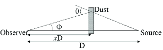
Figure 1: X-ray dust scattering geometry.

The details of X-ray dust scattering can be found in Van de Hulst (1957), Overbeck (1965), Tr$\mathrm{\ddot{u}}$mper & Sch$\mathrm{\ddot{o}}$nfelder (1973), Smith & Dwek (1998). Here we only discuss the single scattering because of the low halo fraction of Cyg X-1 (Xiang, Zhang & Yao 2005). As shown in Fig. 1, the X-ray source is located at a distance of $\mathit{D}$. The dimensionless number $\mathit{x}$ is the fraction of the distance of scattering and that of the source from us. So the lag time of scattered photons at $\mathit{x}$ can be expressed as

$$t_{\mathrm{Delay}}(\phi,x)=(\frac{x}{\cos\phi}+\sqrt{(1-x)^{2}+(x\tan\phi)^{2}}-1)\times\frac{D}{c}.$$ (1)

Let $\mathit{L(t)}$ denotes the luminosity of the source at the location of the source, the observed halo intensity at different observational angle $\phi$ is given by

$$I(\phi,t)=\int_{0}^{1}{{\mathrm{d}}x}\times{D}\times\frac{L(t-t_{\mathrm{Delay}}(\phi,x))\times{\rho(x)}}{(1-x)^{2}\times 4{\pi}D^{2}}\times\frac{\mathrm{d}\sigma(\theta)}{\mathrm{d}\Omega},$$ (2)

here the scattering cross section $\frac{\mathrm{d}\sigma(\theta)}{\mathrm{d}\Omega}$ depends on the energy of the X-ray photon and the radius of the dust grain. $\rho(x)$ is the density of the dust grain at $\mathit{x}$. From Equation 2, the light curve of the halo is delayed and broadened from that of the source.

We can study the delay property directly with the cross-correlation method. The definition of cross-correlation coefficient is given by

$$c(\Delta t)=\frac{1}{N-\arrowvert{\Delta t}\arrowvert}\sum_{t=0}^{N-\arrowvert{\Delta t}\arrowvert-1}(L_{h}(t+\Delta t)-\mu_{h})(L_{s}(t)-\mu_{s}),$$ (3)

here $\mathit{L_{s}}$ and $\mathit{L_{h}}$ are the light curves of the X-ray source and halo (at a given observational angle $\phi$) in the same energy band. $\mu_{s}$ and $\mu_{h}$ are the average values of $\mathit{L_{s}}$ and $\mathit{L_{h}}$ respectively.

3 Data analysis and Simulation

With the long exposure time and the strong variability, Cyg X-1 becomes the first target for our analysis using the cross-correlation. This source was observed with Chandra HETG/ACIS-S for 47 ks on 2003 April 19 (ObsID 3814). We processed the data using the CIAO version 3.4 and the CALDB version 3.4.1. We first searched for point sources around Cyg X-1 using the tool WAVDETECT of CIAO to check whether there are some other point sources which will contaminate the light curve of the halo. The search results show that there is no other bright point source within the diameter of 80^′′ around the position of Cyg X-1 during this observation. Because the halo intensity is sensitive to the energy of photons, therefore we divide the data into three energy bands: below 1 keV (band I), 1 keV$\sim$3 keV (band II), and above 3 keV (band III).

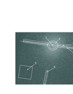
Figure 2: Chandra ACIS-S image of Cyg X-1. The point source of this observation, shown by area 1, has no photons recorded because of the pileup. The annulus 2 shows the area for the annulus of 25^′′. The box 4 is the streak area and the box 3 is the background for the streak area. The box 5 is the background for the data of annuli. The box 6 is a grating arm.

The ACIS-S was in the 1024 pix $\times$ 512 pix mode with a 1.74 seconds frame time during this observation. The zeroth-order data of this observation suffered severe pileup (as shown in Fig. 2), therefore we extracted the light curve of point source from the zero-order streak which is caused by the charge transfer process of the CCD (Smith, Edgar & Shafer 2002), as the true light curve of Cyg X-1. We extract the photons from two 200 pix $\times$ 10 pix boxes (area 4 in Fig. 2) in the streak area but far away from the position of Cyg X-1 to avoid the influence of small angle scattering photons. At the same time, we take the photons of the same area near the streak (area 3 in Fig. 2) as the background for the streak photons. The time bin width, which we use to extract the light curves in the whole analysis, is 100 seconds. The background of the field of view is taken from a box of 100 pix $\times$ 100 pix (area 5 in Fig. 2), far away from the position of Cyg X-1 in the field of view. After making the annuli from 5^′′ to 100^′′ with a bin step of 5^′′ (like annulus 2 in Fig. 2) and subtracting the expected background counts, we can extract the photons from those annuli and obtain the light curves for each observational angle. After extracting all light curves, we make cross-correlation curves between the light curves of the halo and the light curve of the source.

However, the light curves of annuli suffer from contamination of the center point source due to the PSF of the X-ray telescope. Therefore, we must know the exact fraction of photons in the halo from the effect of PSF and subtract them properly. The effect of PSF can be acquired in two different ways: 1) MARX simulation; 2) the observations of point sources with negligible pileup and halo contamination. The simulation is as follows: First we use Sherpa to produce a spectrum file for ChaRT according to the parameters acquired from the observation data we used in this work (Xiang, Zhang & Yao 2005). Then we use ChaRT and MARX to create the simulated observation. The simulated observation has the same location in ACIS with the real observation of Cyg X-1. Following the same routine with Cyg X-1 data used before, we extract the simulated data and obtain the photon distribution at each pixel. For method 2), the PSF fraction comes from the observation of PKS 2155-40. This source is known as not affected by halo photons because of low hydrogen column density (Predehl & Schmitt 1995). The process of extracting the fraction of PSF is the same as that we extract from the observation of Cyg X-1 and the data of the simulation.

4 Results

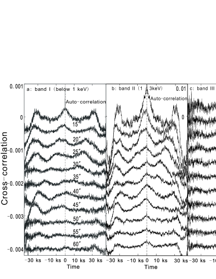
Figure 3: Cross-correlation curves of Cyg X-1 in band I (below 1 keV), band II (1$\sim$3 keV) and band III (above 3 keV). The top curve is the auto-correlation of the light curve of the source; all other curves are the cross-correlation curves from 15^′′ to 60^′′ with a step of 5^′′. For clarity, the cross-correlation coefficients have been lowered by a same amount (0.0004 for panel (a) and 0.004 for panel (b) and 0.003 for panel (c)) successively for each curve. Panel (b) shows obvious contamination of PSF in the center of all of the cross-correlation curves, indicated by the sharp peaks marked by the dashed line. Panel (a) suffers from less contamination because of the higher scattering cross section and narrower profile of PSF below 1 keV. Panel (c) shows more contamination than the other two band.

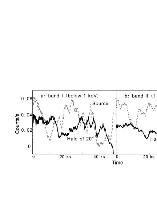
Figure 8: Light curve of the source and its halo of 20^′′ in band I and band II. The gray dashed line shows the light curve of the source. The black solid line shows the light curve of the halo of 20^′′. Here the influence of PSF have been removed from the light curve of the halo. Both the light curves have been smoothed with a window of 2 ks, in order to suppress the counting fluctuations. A lag of around 8 ks is seen clearly.

We compare the auto-correlation of the source light curve with the cross-correlation between source light curve and halo light curve. In Fig. 3 panel (a) and (b) show two groups of peaks in the auto-correlation curve: the peak at zero lag (Peak‘0’ hereafter) with a FWHM of about 10 ks and the other two peaks about 30 ks from the center (Peak‘+’ for the peak of +30 ks and Peak‘-’ for the -30 ks hereafter). Peak‘0’ is due to the variability of the light curve at a timescale of about 10 ks, as shown in Fig. 8. The other two peaks, i.e., Peak‘+’ and Peak‘-’ are resulted from the two big valleys separated by about 30 ks in the light curve of the point source, as seen in Fig. 8. All these three peaks move together to the left with increasing halo radius in both panel (a) and panel (b) of Figure 3, from about 1 ks to 40 ks corresponding to 5^′′ to 50^′′ respectively. The synchronized left-ward shift of all these three peaks in the cross-correlation curves demonstrate the reliability of the cross-correlation method for studying the X-ray scattering halo. Because Peak‘0’ is more pronounced than Peak‘+’ and Peak‘-’, we only carry out quantitative analysis of the lag time for Peak‘0’ in the following.

Panel (b) shows obvious contamination of PSF in the center of all of the cross-correlation curves, indicated by the sharp peaks marked by the dashed line. Panel (a) suffers from less contamination than panel (b). Panel (c) shows more contamination than the other two band. This phenomenon confirms that the scattering of low energy photons are more efficient than the scattering of high energy photons. It is not unexpected that the lag peaks disappear in band III because of its low count rate and the smaller scattering cross section at high energy could decrease the intensity of the halo.

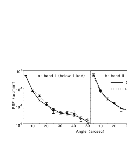
Figure 4: The distribution of PSF in band I and band II. The dotted line shows the observed result of PKS 2155-304. The solid line shows the simulated result. This figure shows that the PSF of low energy photons is narrower than the high energy photons.

The observed and simulated radial profiles of PSF are shown in Fig. 4. The dotted line shows the result of observation of PKS 2155-304 (ObsID 3807). The solid line shows the simulated result. We found that there is no obvious difference between those two results. However, as the locations of the sources of different observations are not always at the same position of the ACIS during the observations of PKS 2155-304, in the following we only use PSF with simulated data, since we can set the positions in simulations.

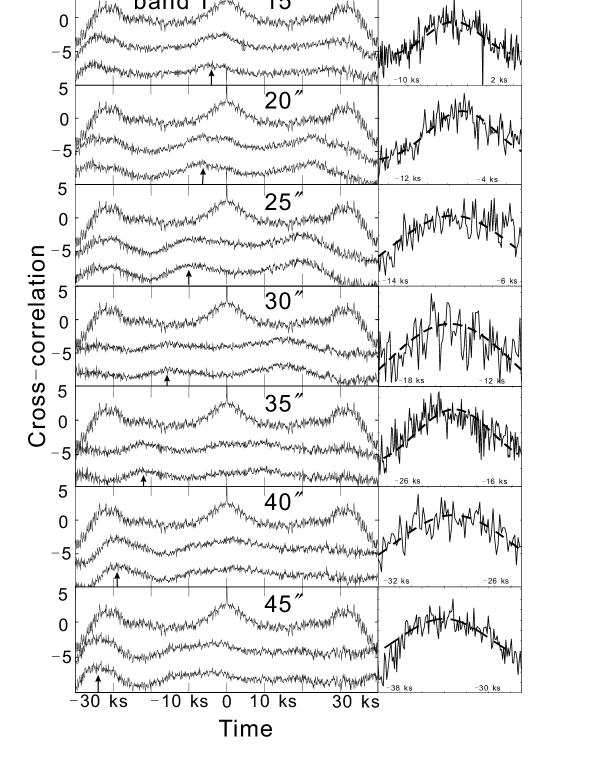
Figure 5: Cross-correlation curves of the halo from 15^′′ to 45^′′ of band I. The top curve in each panel is the auto-correlation of the light curve of the source, the middle curve is the cross-correlation of the light curve of the halo and that of the source, the bottom curve shows the same with the middle curve after removing the contamination of PSF effect. The lower two curves have been lowered by 0.0004 for clarity. The arrows in each panel indicate the lag time at each annulus. The fitting result of the peaks are shown in the right of each sub-figure, with a simple Gaussian function.

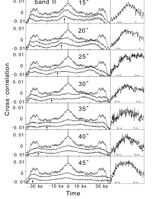
Figure 6: The same as Fig. 5 for band II (1$\sim$3 keV). In this figure, the lower two curves have been lowered by 0.004 for clarity. The lag peaks of 20^′′, 25^′′ and 30^′′ are fitted only with the left data of the peak. The asymmetry of those peak may come from the unremoved contamination of PSF.

The total counts of the source are estimated with the number of streak counts times the exposure factor, which equals to the frame time divided by the total transfer time of the streak area we used ($n_{\mathrm{source}}=n_{\mathrm{streak}}\times 1.74~{}\mathrm{s}/(40~{}\mu\mathrm{s}/\mathrm{pix}\times 400~{}\mathrm{pix})$). After the subtraction of the PSF, the total intensity of the halo from 10^′′ to 100^′′ is about 6.37$\pm$0.04$\%$, which is consistent with Xiang, Zhang & Yao (2005). With the PSF contamination removed, we can then derive the real time lag of each annulus. Fig. 5 and Fig. 6 show the cross-correlation curves of 15^′′ to 45^′′ in band I and band II. The top curve in each panel is the auto-correlation of the light curve of the source, the middle curve is the cross-correlation of the light curve of the halo and that of the source, the bottom curve shows the same with the middle curve after removing the contamination of PSF effect. The lower two curves have been lowered for clarity. The arrows in each panel indicate the lag time at each halo radius. The fitting result of those peaks are shown in the right of each sub-figure, with a simple Gaussian function. The lag peaks of 20^′′, 25^′′ and 30^′′ in Fig. 6 are fitted only with the left data of the peak. The asymmetry of those peaks may come from the unremoved contamination of PSF. In Fig. 5, the cross-correlation curves also show the lag peaks clearly even before the elimination of PSF (the middle curve of each sub-figure in Fig. 5).

As shown in Fig. 5 and Fig. 6, Peak‘+’ in the cross-correlation curves moves to the left, and Peak‘-’ moves out of the cross-correlation curves. The intervals of those peaks in the bottom curve of each panel are always the same as in the auto-correlation, about 30 ks, as expected by applying the cross-correlation method.

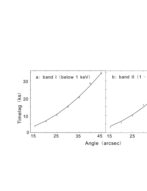
Figure 7: The lag time vs halo radius. Panel (a) shows the result of band I (below 1 keV) and panel (b) shows band II (1$\sim$3 keV). The best fit result is $\mathit{x}$ = 0.876$\pm$ 0.002 for band I and $\mathit{x}$ = 0.872$\pm$ 0.002 for band II. The solid lines show the best fit results. Because of its less contamination of PSF and better fitting, the result of band I is used in this work.

By fitting the Peak‘0’ in each cross-correlation curves, we can get the time lags at each halo radius. The results are shown in Fig. 7. We use a simple dust wall model to fit the different time lag, with an assumption of 2 kpc distance from Cyg X-1 to us (Mirabel $\&$ Rodrigues 2003). Panel (a) shows the result of band I (below 1 keV) and panel (b) shows band II (1$\sim$3 keV). The best fit result is $\mathit{x}$ = 0.876$\pm$ 0.002 for band I and $\mathit{x}$ = 0.872$\pm$ 0.002 for band II. The solid lines show the best fit results. Because of its less contamination of PSF and better fitting, the result of band I is used in this work. The result shows that the dust exists at $\mathit{x}$ = 0.876 $\pm$ 0.002, i.e., 1.752 kpc away from us.

To illustrate the time lag revealed by the cross-correlation method, we plot the light curves of the source and halo together. As shown in Fig. 8, the light curves of the source and the halo at 20^′′ in band I and band II both reveal an obvious lag of about 8 ks, just as the result from Fig. 7. Both the light curves in Fig. 8 have been smoothed with a window of 2 ks, in order to suppress the counting fluctuations.

The width of the dust wall at $\mathit{x}$ = 0.876 can also be estimated from the broadening property of the light curves of the halo. We use a simple model of a dust layer extended from $\mathit{x}$ = 0.876 to both sides along the LOS to simulate the light curves of the halo. With Equation 2, we could obtain the ideal response curve of a delta function with the parameter of the dust layer width of $\mathit{\Delta L}$. After convolving the light curve of the source with the ideal response function, we could produce light curves of the halo at each angle. We define the $\chi^{2}$ by

$$\chi^{2}=\sum_{i}(\frac{n_{\mathrm{i,simu}}-n_{\mathrm{i,obser}}}{\sigma_{\mathrm{i,obser}}})^{2},$$ (4)

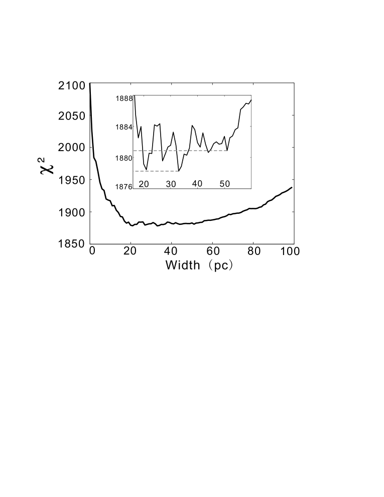
Figure 9: The $\chi^{2}$ distribution vs the width of dust layer $\mathit{\Delta L}$. We use the light curves of band II here because of its high count rates. The minimum $\chi^{2}$ = 1878 with 1664 degrees of freedom. The 90$\%$ confident range is [20, 51] pc, with the $\Delta\chi^{2}$ = 2.71 (Avni 1976).

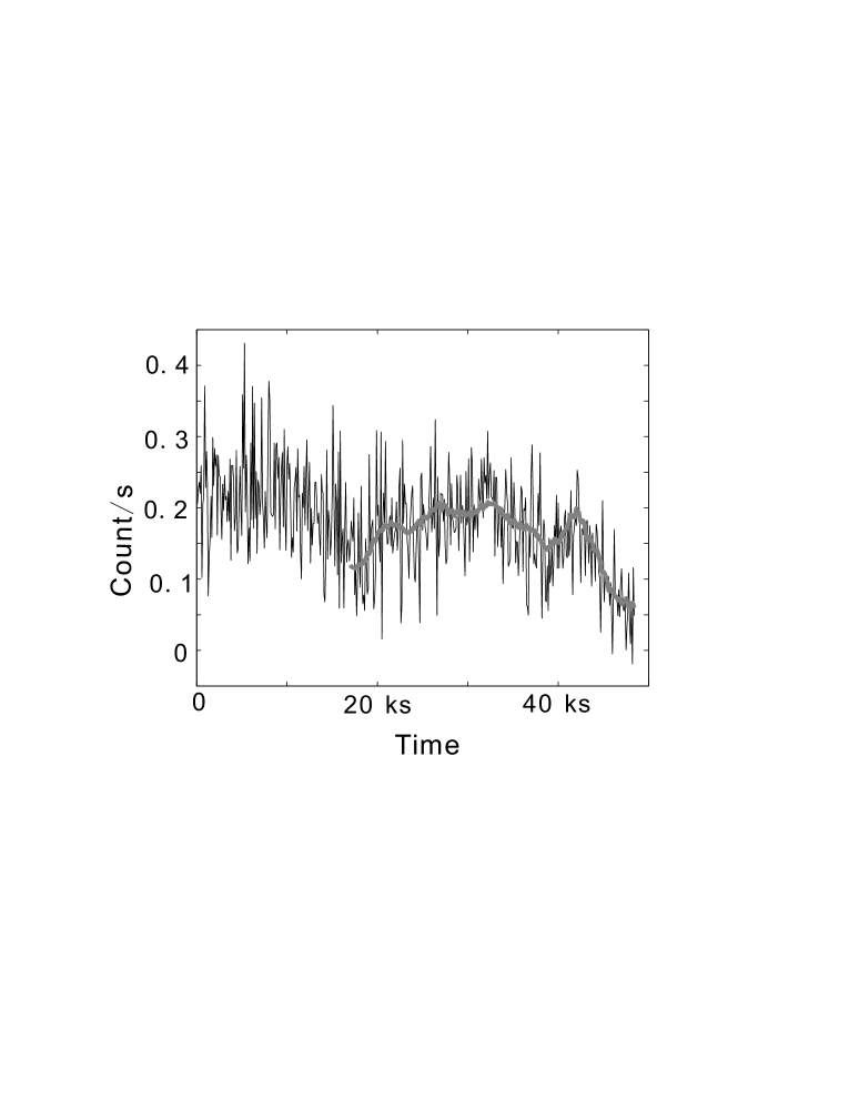
Figure 10: The observed light curve of the halo of 20^′′. The grey line shows the simulated result for $\mathit{\Delta L}$ = 33 pc and $\mathit{x}$ = 0.876. Clearly the simulated light curve resembles the observed light curve quite well. The simulated light curves at each time bin number $\mathit{i}$ is depending on the observational light curve before the time bin number $\mathit{i}$ with a length of the response function because of the convolution process. However, since the light curves are not available before the start of this observation, the initial part of the simulated data of about 16 ks is omitted.

here $\mathit{i}$ is the time bin number including the light curves at each angle. $n_{\mathrm{i,simu}}$ and $n_{\mathrm{i,obser}}$ denote the simulated and observed count rates at each time bin number $\mathit{i}$. $\sigma_{\mathrm{i,obser}}$ denotes the error of observed data at time $\mathit{i}$. We use the observed light curves of band II here because of its high count rates. By comparing the simulated curves with the observed curves, we get a range of the parameter $\mathit{\Delta L}$. As shown in Fig. 9, the minimum $\chi^{2}$ = 1878 with 1664 degrees of freedom. The 90$\%$ confident range is [20, 51] pc, with $\Delta\chi^{2}$ = 2.71 (Avni 1976). We show the simulated light curve of 20^′′ and the observed light curve of 20^′′ in Fig. 10 with $\mathit{x}$ = 0.876 and $\mathit{\Delta L}=33$ pc. Clearly the simulated light curve resembles the observed light curve quite well. The simulated light curves at each time bin number $\mathit{i}$ is depending on the observational light curve before the time bin number $\mathit{i}$ with a length of the response function because of the convolution process. However, since the light curves are not available before the start of this observation, the initial part of the simulated data of about 16 ks (this value means that the scattering happens at $\mathit{x}$ = 0.95, which corresponds to the largest distance the dust layer can reach) is omitted in Fig. 10.

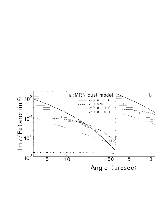
Figure 11: Halo profile of Cyg X-1 in the energy band of 1.0 keV to 5.0 keV (Xiang, Zhang $\&$ Yao 2005). Here we use the MRN dust model (panel a) and WD01 dust model (panel b) with a hydrogen column density of $5.0\times 10^{21}/\mathrm{cm^{2}}$. The dashed line is the result of dust in 0.876. The solid line is the result of dust smooth distributed between $\mathit{x}$ = 0.9 to 1.0. The dotted line is the result of dust smooth distributed between $\mathit{x}$ = 0.0 to 1.0. The dashed dotted line is the result of dust smooth distributed between $\mathit{x}$ = 0 to 0.1. From those curves, we can infer that the fitting of halo surface brightness with MRN or WD01 dust models would lead to a dust concentration near the source.

However, Xiang, Zhang $\&$ Yao (2005) fitted the halo surface brightness of 17 sources with two dust grain models and claimed that most of the dusts along the LOS of Cyg X-1 are located at $\mathit{x}$ larger than 0.9. To explain this difference, we plot the halo surface brightness of Cyg X-1 again. As shown in Fig. 11, we find that the halo surface brightness cannot be fit with the dust distribution in which the dusts are located at $\mathit{x}$ = 0.876 or dust uniformly distributed between $\mathit{x}$ = 0 and $\mathit{x}$ = 1. The halo surface brightness of Cyg X-1 of Xiang, Zhang $\&$ Yao (2005) would lead to a dust concentration near the source with the MRN (Mathis, Rumpl & Nordsiech 1977) dust grain model or the WD01 (Weingartner $\&$ Draine 2001) model. Witt, Smith, $\&$ Dwek (2001) fitted the halo surface brightness by the MRN dust grain model and a smoothed dust distribution. They found that the halo of Nva Cygni 1992 cannot be fitted by the MRN model unless the model is modified with the maximum radius of dust grain extending to 2 $\mu$m. Valencic and Smith (2008) also argued that the radius of dust grain of MRN or WD01 model are not realistic. They tested the MRN and WD01 dust grain models using the UV extinction and X-ray halos along the LOS toward X Per. Both models provided reasonable fits to the UV extinction and X-ray halos but cannot do so while respecting the elemental abundance constraints. Furthermore, the abundances and $N_{H}$ required to reproduce the observations in these two regimes are not consistent with each other, reflecting the fact that X-ray regime constraints were not taken into account when the grain size distributions were constructed, and thus the models are incomplete. The MRN model has long been known to be unphysical and WD01 model was simply never designed with the X-ray regime, as pointed out by Valencic and Smith (2008). All results cast doubt on those dust models. We therefore conclude that the two commonly accepted models of dust grain size distribution must be modified significantly before they are used in the X-ray regime.

5 Summary and Discussion

We applied the cross-correlation method to the light curves of Cyg X-1 and found the photons of the halo significantly lag from that of the source itself. This time lag implies a dust concentration at $\mathit{x}$ = 0.876 $\pm$ 0.002 with the source distance of 2.0 kpc. But the lag disappears when the energy of photons exceeds 3 keV in this analysis: both the low count rate and the smaller scattering cross section could decrease the intensity of halo. By the broadening property of light curves, we derived a dust width of $\mathit{\Delta L}=33_{-13}^{+18}$ pc.

The cross-correlation method can avoid assumptions of photon energy, dust grain radius, dust distribution, scattering cross section and so on. Therefore the time lag derived by this method only rests on pure geometry, but not connected at all with the parameters of dust grain. Consequently, our results can be used to determine the parameter of the dust grain models in the future, when combined with the spatial distribution of the X-ray dust scattering halo; currently no dust grain model can describe simultaneously the time lag and spatial distribution of X-ray dust scattering halo. Besides, if the position of the scattering dust cloud is known from other methods, we can also derive the distances of the sources with this cross-correlation method.

The origin of this dust layer is still unknown. There may exists a molecular cloud. The width of $\mathit{\Delta L}=33_{-13}^{+18}$ pc is also consistent with a typical molecular cloud. We searched for all of the known molecular clouds but failed to find a counterpart for this dust layer. Another possibility is that there is a super-bubble around Cyg X-1, and $\mathit{x}$ = 0.876 $\pm$ 0.002 is just the edge along the LOS. This hypothesis is consistent with Gallo et al. (2003) who found a low density region of about 5 pc around Cyg X-1. We also did not find longer time lags corresponding to the region of about 5 pc to the source in cross-correlation curves or light curves, indicating there is very little dust between $\mathit{x}$ = 0.876 and the center source along the LOS. We also cannot constrain well the dust distribution between the inferred dust wall and the observer. This is because that the scattered photons from any dust in this region are not significant for the halo at smaller angular distances. The only qualitative statement about the dust between the wall and the observer is that the dust density outside the wall must be much lower than in the wall; otherwise shorter lags should have been detected in the halo’s light curve. Finally, we did not intend to derive the dust and neutral hydrogen column density, because the dust grain size distribution and scattering cross section are not well understood yet.

References

- (1) Avni, Y., 1976, ApJ, 210, 642
- (2) Catura, R. C. 1983, ApJ, 275, 645
- (3) Gatto, E. et al, 2005, Nature, 436, 819
- (4) Hu, J., Zhang, S. N., & Li, T. P. 2004, ApJ, 614, L45
- (5) Mathis, J. S., Rumpl, W., & Nordsieck, K. H. 1977, ApJ, 217, 425 (MRN)
- (6) Mauche, C. W., & Gorenstein, P. 1986, ApJ, 302, 371
- (7) Mirabel, I. F., & Rodrigues, I. 2003, Science, 300, 1119
- (8) Overbeck, J. W. 1965, ApJ, 141, 864
- (9) Predehl, P., Burwitz, V., Paerels, F., & Trmper, J. 2000, A&A, 357, L25
- (10) Predehl, P., & Schmitt, J. H. M. M. 1995, A&A, 293, 889
- (11) Rolf, D. P. 1983, Nature, 302, 46
- (12) Shao, L., & Dai, Z. G. 2007, ApJ, 660, 1319
- (13) Shao, L., Dai, Z. G., & Mirabal, N. 2008, ApJ, 675, 507
- (14) Smith, R. K., & Dwek, E. 1998, ApJ, 503, 831
- (15) Smith, R. K., Edgar, R. J., & Shafer, R. A. 2002, ApJ, 581, 562
- (16) Trmper, J., & Schnfelder, V. 1973, A&A, 25, 445
- (17) Valencic, L. A., & Smith, R. K. 2008, ApJ, 672, 984
- (18) van de Hulst, H.C. 1957, Light Scattering by Small Particle (New York: Dover)
- (19) Vaughan, S., et al. 2004, ApJL, 603, L5
- (20) Vaughan, S., et al. 2006, ApJ, 639, 323
- (21) Weingartner, J. C., & Draine, B. T. 2001, ApJ, 548, 296 (WD01)
- (22) Witt, A., Smith, R. K., & Dwek, E. 2001, ApJ, 550, 201
- (23) Xiang, J. G., Lee, J. C., & Nowak, M. A. 2007, ApJ, 660, 1309
- (24) Xiang, J. G., Zhang, S. N., & Yao, Y. S. 2005, ApJ, 628, 769
- (25) Yao, Y. S., Zhang, S. N., Zhang, X. & Feng, Y. 2003, ApJ, 59, L43