Three-particle cumulant Study of Conical Emission

Abstract

We discuss the sensitivity of the three-particle azimuthal cumulant method for a search and study of conical emission in central relativistic $A+A$ collisions. Our study is based on a multicomponent Monte Carlo model which include flow background, Gaussian mono-jets, jet-flow, and Gaussian conical signals. We find the observation of conical emission is hindered by the presence of flow harmonics of fourth order ( $v_{4}$) but remains feasible even in the presence of a substantial background. We consider the use of probability cumulants for the suppression of 2^nd order flow harmonics. We find that while probability cumulant significantly reduce $v_{2}^{2}$ contributions, they also complicate the cumulant of jets, and conical emission. The use of probability cumulants is therefore not particularly advantageous in searches for conical emission. We find the sensitivity of the (density) cumulant method depends inextricably on strengths of $v_{2}$, $v_{4}$, background and non-Poisson character of particle production. It thus cannot be expressed in a simple form, and without specific assumptions about the values of these parameters.

I Introduction

Observations of away-side dip structures in two-particle correlations measured in $Au+Au$collisions at $\sqrt{s_{NN}}=200$ GeV have stimulated renewed interest in the notion of conical emission. The passage of a parton through dense matter at speeds greater than the speed of sound is predicted to lead to the production of a Mach shock wake resulting in conical emission pattern that may explain the observed two-particle correlations Stoecker76 ; Stoecker05 ; JRuppert05 ; RupperMuller05 ; SolanaShuryak05 ; RenkRuppert06 ; Heinz06 ; Stocker07 ; RenkRupper07 ; MullerQM08 ; BBetz08 . Identification of Mach cone is of great interest because it could provide an experimental determination of the speed of sound in the dense medium produced in high energy $A+A$ collisions SolanaShuryak05 ; Mukherjee07 . A sonic boom is also expected for a heavy quark propagation based on Ads/CFT calculation Gubser08 . Cerenkov radiation produced by a superluminal parton traversing a dense medium is expected to generate a similar signature Dremin79 ; Dremin81 ; Dremin06 ; KochMajumber05 ; MajumderMuller06 . However, other production mechanisms have been proposed to explain the two-particle correlation data. These include large angle gluon radiation Vitev05 ; PolosaSalgado05 , path length effects Hwa05 , collective flow, and jet deflection Armesto04 ; Salgado05a ; RenkRuppert07_PLB646 ; RenkRuppertPRC2007 ; Voloshin05 ; Hwa05_PRC74 .

Three-particle correlation measurements were proposed to gain further insight in the particle production mechanism leading to the away-side deep structure seen in two-particle correlations. Various methods have been suggested and are currently pursued to carry such analyses. A number of these analyses are carried out using a flow $+$ signal decomposition, i.e. an adhoc flow background is assumed and subtracted based on the ZYAM approximation Holzmann05 ; Ajitanand06 ; Ulery06_774 ; Ulery06a ; Ulery06b ; Ulery06c ; Ajitanand06_774 ; Ulery07 ; CeresQM06 ; Kniege07 ; Ajitanand07 . Note however that, as Borghini pointed out, momentum conservation can have a significant impact on two- and three-particle correlations Borghini06 . The magnitude of momentum conservation effects is however difficult to estimate as discussed recently by Chajecki et al. Lisa08 . A cumulant based method was proposed by the author Pruneau06 and is also used by the STAR collaboration Pruneau06a to search for conical emission. This method presents the advantage that the extraction of a three-particle signal does not require any model assumptions. Obviously, one can also carry a model based decomposition of the extracted three-particle signal, i.e. the cumulant, to estimate its various components, and seek evidence for conical emission.

In this work, we further study the properties of the three-particle cumulant observable first proposed in Ref. Pruneau06 for a search for conical emission, and studies of particle production dynamics. Three particles correlations, designed to search for conical emission, use a high $p_{t}$ particle as a jet tag. The azimuthal angle of this high $p_{t}$ particle should approximately correspond to the direction of the parton initiating the tagged jet. It is further assumed the emission of this parton is surface biased, and directed outward, approximately normal to the surface of the medium. The direction of the high-$p_{t}$ particle thus provides a reference to study the propagation of the away-side parton initiating the second jet. Estimates of the sound velocity in the quark gluon plasma suggest the wake produced by a high energy parton should produce particle emission at a Mach angle of the order of one radian relative to the parton direction SolanaShuryak05 . This corresponds to enhanced particle emission at angles of order 2 radian with respect to the high-$p_{t}$ jet tag. An unsuppressed away-side jet should on the other hand lead to particle emission at an angle of approximately $\pi$ relative to the jet tag. Deflection or radial flow effects should produce a broadening of the away-side jet relative to the high-$p_{t}$ tag.

We define the notation and variables used in this paper in Section II. We next discuss, in Section III, simple models of particle production including di-jets, flow, conical emission, as well as the effects of differential jet quenching, hereafter called jet-flow. We show in Sec. III.2 that in the case of Poisson statistical particle production, the three particle cumulant (hereafter noted 3-cumulant) associated with azimuthal anisotropy reduces to a simple expression involving only non-diagonal Fourier terms. In view of the large values of elliptic flow $v_{2}$ observed in $A+A$ collisions at RHIC, one expects the leading non-diagonal term should be of order $v_{2}v_{2}v_{4}$. However, one finds experimentally that fluctuations in the number of produced particles are non-Poissonian. We thus consider in Sec. IV the impact of such non-Poissonian fluctuations, and find they imply the presence of sizable $v_{2}^{2}$ terms in the three-cumulant that may complicate the observation of conical emission signals. We show the $v_{2}^{2}$ terms may however be suppressed if one adopts a modified version of the cumulant based on probability densities rather than number densities, and suggest this modified cumulant as an alternative means of studying three-particle correlations.

The cumulant method is a relatively complicated analysis technique, which may in principle be sensitive to various instrumental effects. We discuss a specific implementation of the method based on normalization to single particle distributions in Sec. V. We show, based on the conical emission model introduced in Sec. VI and an adhoc parameterization of the detection efficiency, that normalization by single particle distributions leads to a robust analysis technique.

A key issue in the search for conical emission is the sensitivity of the method used to extract the three- particle correlation information. We discuss, in Section VI, the sensitivity of the cumulant method based on a simple jet and conical emission Monte-Carlo model.

Our conclusions are summarized in Section VII.

II Definitions and Notation

The conical emission search method introduced in Ref. Pruneau06 is based on the observation of three-particle densities as a function of the relative azimuthal angles between the measured particles. The presence of three-particle correlations, and possible signal for conical emission is extracted using the 3-cumulants. A high $p_{t}$ particle is used as a jet tag, and proxy for determination of the direction of the jet. Two lower $p_{t}$ particles are used to probe the structure of the near-side jet (i.e. the jet singled out by the high-$p_{t}$ tag particle) and search for conical emission on the away-side. The jet tag is herein referred as particle 1 while the two associates are labeled as particles 2 and 3. The three particles are detected in the collision transverse plane at angles $\varphi_{1}$, $\varphi_{2}$, and $\varphi_{3}$ relative to some arbitrary reference frame. The single, two-, and three- particle densities are noted as follows:

$$\rho_{1}(\varphi_{i}) = dN_{1}/d\varphi_{i}$$ (1)

$$\rho_{2}(\varphi_{i},\varphi_{j}) = dN_{2}/d\varphi_{i}d\varphi_{j}$$

$$\rho_{3}(\varphi_{i},\varphi_{j},\varphi_{k}) = dN_{3}/d\varphi_{i}d\varphi_{j}d\varphi_{k}$$

where the indices $i$, $j$, and $k$ take values 1, 2, and 3.

The three-particle or triplet density, $\rho_{3}$, corresponds to the average number of particle triplets observed per collision. The particles of a given triplet are however not necessarily correlated. Indeed, the three particles may originate from one, two, or three (distinct or not) production processes (e.g. radial flow, elliptic flow, resonance decay, jets, Mach cone, etc). Cumulants are designed to extract the three-particle correlation component from the three-particle density. They were first discussed in the context of particle physics (see for instance Berger ; Carruthers ) and are now used in a variety of analyses. It is the purpose of this work to study specific aspects of the cumulant method introduced in Pruneau06 for studies of the shape and strength of the signal expected from different types of processes and to characterize the robustness and sensitivity of the method.

The 2- and 3-cumulants $C_{2}$ and $C_{3}$ are defined as follows:

$$C_{2}(\varphi_{i},\varphi_{j}) \equiv \rho_{2}(\varphi_{i},\varphi_{j})-\rho_{1}(\varphi_{i})\rho_{1}(\varphi_{j})$$

$$C_{3}(\varphi_{i},\varphi_{j},\varphi_{k}) \equiv \rho_{3}(\varphi_{i},\varphi_{j},\varphi_{k})-\rho_{2}(\varphi_{i},\varphi_{j})\rho_{1}(\varphi_{k})$$

$$- \rho_{2}(\varphi_{i},\varphi_{k})\rho_{1}(\varphi_{j})-\rho_{2}(\varphi_{j},\varphi_{k})\rho_{1}(\varphi_{i})$$

$$+ 2\rho_{1}(\varphi_{i})\rho_{1}(\varphi_{j})\rho_{1}(\varphi_{k})$$

As described in Ref. Pruneau06 the two-, three-particle densities and cumulants are straightforwardly corrected for detector inefficiencies provided the three- and two-particle detection efficiencies may be factorized as products of respectively two and three single particle efficiencies. The robustness of this correction procedure is discussed in Sec. V on the basis of Monte Carlo simulations.

Correlation functions in terms of relative angles, $C_{3}(\Delta\varphi_{ij},\Delta\varphi_{ik})$, are formally obtained by integration of the cumulants $C_{3}(\varphi_{i},\varphi_{j},\varphi_{k})$ with constraints $\Delta\varphi_{ij}=\varphi_{i}-\varphi_{j}$.

$$C_{3}(\Delta\varphi_{ij},\Delta\varphi_{ik}) = \int{C_{3}(\varphi_{i},\varphi_{j},\varphi_{k})}$$

$$\times \delta(\Delta\varphi_{ij}-\varphi_{i}+\varphi_{j})$$

$$\times \delta(\Delta\varphi_{ik}-\varphi_{i}+\varphi_{k})d\varphi_{i}d\varphi_{j}d\varphi_{k}$$

In practice, this is accomplished by binning $C_{3}(\varphi_{i},\varphi_{j},\varphi_{k})$ and $C_{3}(\Delta\varphi_{ij},\Delta\varphi_{ik})$ into arrays (e.g. 72x72x72 and 72x72 respectively) and summing the elements of $C_{3}(\varphi_{i},\varphi_{j},\varphi_{k})$ to obtain $C_{3}(\Delta\varphi_{ij},\Delta\varphi_{ik})$ as follows.

$$C_{3}(p,q)=\sum\limits_{i,j,k=1}^{72}C_{3}(i,j,k)\delta(p-i+k)\delta(q-i+k)$$ (4)

for $p$=1, …,72; $q$=1, …,72. Given the finite statistics, and the large memory requirement implied by three-dimensional arrays used in this type of analysis, care must be taken when binning the densities. We found the use of 72 bins, for analysis of data samples collected e.g. by the STAR experiment StarNim ; StarC308 enables sufficient angular resolution and statistical accuracy.

III Signal Modeling

We use specific models for jet, di-jet production, collective flow, and conical emission signals in order to assess the sensitivity of the cumulant method for a search of conical emission. The models are described in the following sub-sections while our study of the sensitivity of the cumulant method is presented in Section VI.

III.1 Di-Jet Production

Jet production is characterized by the emission of particles in a cone (in momentum space) centered on the direction of the parton that produces the jet. We consider di-jet production restricted to central rapidities (near $90^{o}$ relative to the beam direction), and assume the number of di-jet per event in the acceptance of the detector, J, varies event-by-event. The intra-jet particle multiplicity depends on the jet energy, but is order three (3) at RHIC energy CDF_JET . We consider back-to-back jets in azimuth, but possibly different longitudinal momenta. We denote the number of jet particles measured within each kinematics cut ”$i$” as $A_{i}$. and $A_{i}^{\prime}$ respectively for the near and away side jets. The emission of particles relative to the jet axis is described by a probability distribution $P_{assoc}(\theta)$, where $\theta$ is the angle between the particle momentum and the momentum vector of the parton originating the jet. Projection of this distribution in the transverse plane leads to a probability distribution, $P_{J}(\varphi)$, function of the azimuthal angle, $\varphi$, between the parton and the particle direction. Following Pruneau06 , we further simplify the jet model and use a Gaussian azimuthal profile, $G_{2}(\varphi_{i}-\phi_{\alpha};\sigma_{i})$ with $G_{2}(x;\sigma)\equiv\left({\sqrt{2\pi}\sigma}\right)^{-1}\exp\left({-{{x^{2}}\mathord{\left/{\vphantom{{x^{2}}{2\sigma^{2}}}}\right.\kern-1.2pt}{2\sigma^{2}}}}\right)$ where $\varphi_{i}$, $\phi_{\alpha}$, and $\sigma_{i}$ are the emission angle (in the lab frame) of measured particles, the emission angle of the parton, and the width of the jet, respectively. For this illustrative model, we assume the emission angle and the jet multiplicity are not correlated to the collision reaction plane. We further assume one can decouple the number of particles, in the measured kinematic range of interest, from the jet profile. The number of jets, their multiplicity, and directions are not known, and must therefore be averaged out. The 3-particle jet cumulant is given by the following expression.

$$C_{3}^{Jet}(\Delta\varphi_{12},\Delta\varphi_{13}) = (2\pi)^{-1}\left\langle J\right\rangle\left\{\begin{array}[]{l}\left\langle{A_{1}A_{2}A_{3}}\right\rangle G_{3}(\Delta\varphi_{12},\Delta\varphi_{13};\sigma_{1},\sigma_{2},\sigma_{3})\\ +\left\langle{A_{1}A_{2}A^{\prime}_{3}}\right\rangle G_{3}(\Delta\varphi_{12},\Delta\varphi_{13}-\pi;\sigma_{1},\sigma_{2},\sigma^{\prime}_{3})\\ +\left\langle{A_{1}A^{\prime}_{2}A_{3}}\right\rangle G_{3}(\Delta\varphi_{12}-\pi,\Delta\varphi_{13};\sigma_{1},\sigma^{\prime}_{2},\sigma_{3})\\ +\left\langle{A_{1}A^{\prime}_{2}A^{\prime}_{3}}\right\rangle G_{3}(\Delta\varphi_{12}-\pi,\Delta\varphi_{13}-\pi;\sigma_{1},\sigma^{\prime}_{2},\sigma^{\prime}_{3})\\ \end{array}\right\}$$ (9)

$$+ (2\pi)^{-2}\left({\left\langle{J(J-1)}\right\rangle-\left\langle J\right\rangle^{2}}\right)\left\{\begin{array}[]{l}\left\langle{A_{1}A_{2}}\right\rangle\left\langle{A_{3}+A^{\prime}_{3}}\right\rangle G_{2}(\Delta\varphi_{12};\sigma_{12})\\ +\left\langle{A_{1}A_{3}}\right\rangle\left\langle{A_{2}+A^{\prime}_{2}}\right\rangle G_{2}(\Delta\varphi_{13};\sigma_{13})\\ +\left\langle{A_{2}A_{3}}\right\rangle\left\langle{A_{1}}\right\rangle G_{2}(\Delta\varphi_{13}-\Delta\varphi_{12};\sigma_{23})\\ +\left\langle{A_{1}A^{\prime}_{2}}\right\rangle\left\langle{A_{3}+A^{\prime}_{3}}\right\rangle G_{2}(\Delta\varphi_{12}-\pi;\sigma^{\prime}_{12})\\ +\left\langle{A_{1}A^{\prime}_{3}}\right\rangle\left\langle{A_{2}+A^{\prime}_{2}}\right\rangle G_{2}(\Delta\varphi_{13}-\pi;\sigma^{\prime}_{13})\\ +\left\langle{A^{\prime}_{2}A^{\prime}_{3}}\right\rangle\left\langle{A_{1}}\right\rangle G_{2}(\Delta\varphi_{13}-\Delta\varphi_{12};\sigma^{\prime}_{23})\\ \end{array}\right\}$$

$$+ (2\pi)^{-3}\left({\left\langle{J(J-1)(J-2)}\right\rangle-3\left\langle{J(J-1)}\right\rangle\left\langle J\right\rangle+2\left\langle J\right\rangle^{3}}\right)\left\langle{A_{1}}\right\rangle\left\langle{A_{2}+A^{\prime}_{2}}\right\rangle\left\langle{A_{3}+A^{\prime}_{3}}\right\rangle$$

with

$$G_{3}(x_{1},x_{2};\sigma_{1},\sigma_{2},\sigma_{3})=\left(2\pi\right)^{-1}\sigma_{1,2,3}^{-2}\\ \times\exp\left({-{{\left({\sigma_{3}^{2}x_{1}^{2}+\sigma_{2}^{2}x_{2}^{2}+\sigma_{1}^{2}(x_{1}-x_{2})^{2}}\right)}\mathord{\left/{\vphantom{{\left({\sigma_{{}_{3}}^{2}x_{1}^{2}+\sigma_{{}_{2}}^{2}x_{2}^{2}+\sigma_{{}_{1}}^{2}(x_{1}-x_{2})^{2}}\right)}{2\sigma_{1,2,3}^{2}}}}\right.}{2\sigma_{1,2,3}^{2}}}}\right)$$ (17)

where $x_{ij}=x_{i}-x_{j}$, $\sigma_{ij}^{2}=\sigma_{i}^{2}+\sigma_{j}^{2}$ and $\sigma_{i,j,k}^{4}=\sigma_{i}^{2}\sigma_{j}^{2}+\sigma_{i}^{2}\sigma_{k}^{2}+\sigma_{j}^{2}\sigma_{k}^{2}$. Note $G_{3}$ is defined such its integral over $x_{1}$ and $x_{2}$ is unity. The coefficient $\left\langle J\right\rangle$ determines the average number of jets per event. Coefficients $A_{1}$, $A_{2}$, $A_{3}$ describe the number of particles associated with the near side jet, while $A^{\prime}_{1}$, $A^{\prime}_{2}$, $A^{\prime}_{3}$ correspond to the number of particles associated with the away side jet observed within the kinematic cuts used for the study of the correlation functions. We note that if the number of jets, J, in each event is determined by a Poisson process, then one has $\left\langle{J(J-1)}\right\rangle=\left\langle J\right\rangle^{2}$ and $\left\langle{J(J-1)(J-2)}\right\rangle-3\left\langle{J(J-1)}\right\rangle-2\left\langle J\right\rangle^{3}=0$. The constant term, and the terms containing a 2-particle dependence in $G_{2}$ then vanish in the above expression. The jet 3-cumulant is plotted in Figure 1, in arbitrary amplitude units, for $\sigma_{1}=0.15$, $\sigma_{2}=\sigma_{3}=0.2$, $\sigma^{\prime}_{2}=\sigma^{\prime}_{3}=0.4$, $\left\langle J\right\rangle=1$, $A_{1}=1$, $A_{2}=A_{3}=2$, and $A^{\prime}_{2}=A^{\prime}_{3}=1$. We further assume for simplicity that $\left\langle A_{i}A_{j}\right\rangle=\left\langle A_{i}\right\rangle\left\langle A_{j}\right\rangle$ and $\left\langle A_{1}A_{2}A_{3}\right\rangle=\left\langle A_{1}\right\rangle\left\langle A_{2}\right\rangle\left\langle A_{3}\right\rangle$ although it is unlikely realized in practice. Panel (a) presents the cumulant for the Poissonian case, whereas panel (b) displays a non-Poissonian case for which ${{\left\langle{J(J-1)}\right\rangle-\left\langle J\right\rangle^{2}}\mathord{\left/{\vphantom{\left({\left\langle{J(J-1)}\right\rangle-\left\langle J\right\rangle^{2}}\right){\left\langle J\right\rangle^{2}}}}\right.\kern-1.2pt}{\left\langle J\right\rangle^{2}}}=0.05$. The peak centered at $\Delta\varphi_{12}=\Delta\varphi_{13}=0$ corresponds to two particles associated with the high $p_{t}$ particle, and is referred to as the near side jet peak. Secondary peaks at $(0,\pi)$, $(\pi,0)$, and $(\pi,\pi)$ correspond to one or both the associates being detected on the away side. The bands seen in Figure 1 (b) stem from the non-zero two-particle contributions to the 3-cumulant for non-Poissonian events. Various effects may alter the strength and shape of the jet correlations. Interactions of the parton with the medium may produce jet broadening, and deflection. Given jet emission is expected to be surface biased in $A+A$ collisions (in view of recent measurements of small $R_{AA}$, and the disappearance of the away side jet WhitePapers ), one expects the near side peak to have similar width in $A+A$ collisions as in $p+p$ collisions, while the away-side peak should be broader. One might also observe additional broadening along $\Delta\varphi_{12}$, and $\Delta\varphi_{13}$ due to parton scattering, and radial flow.

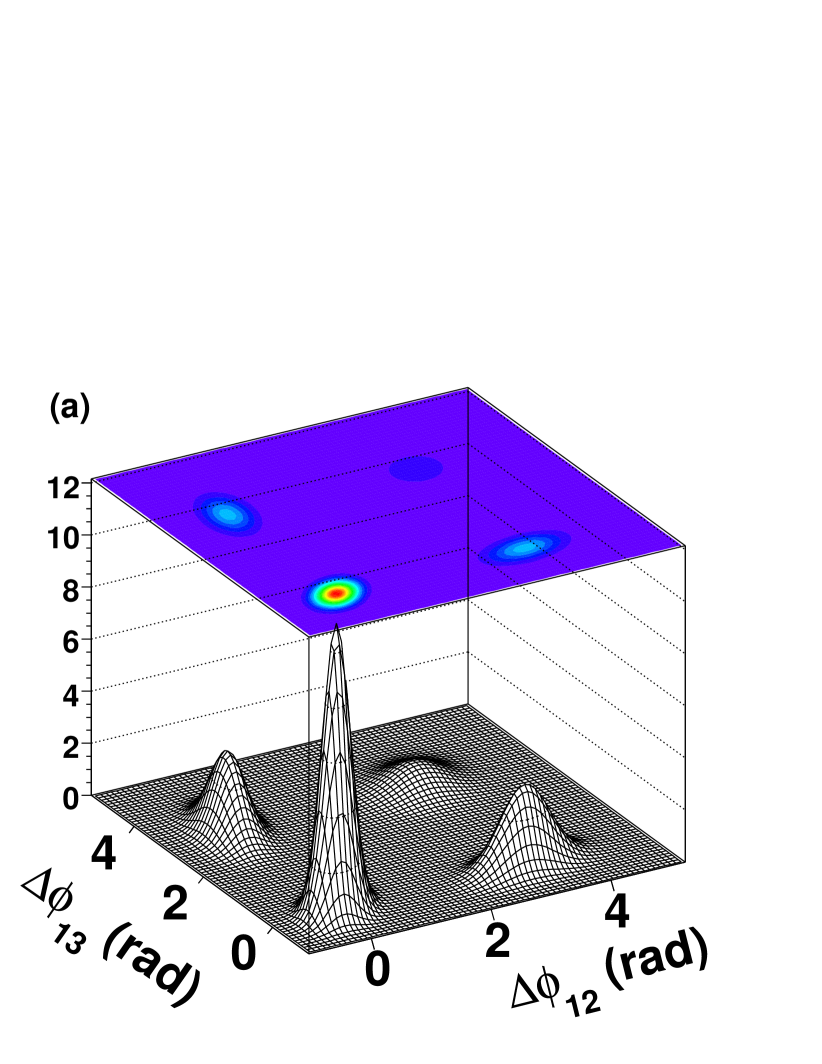
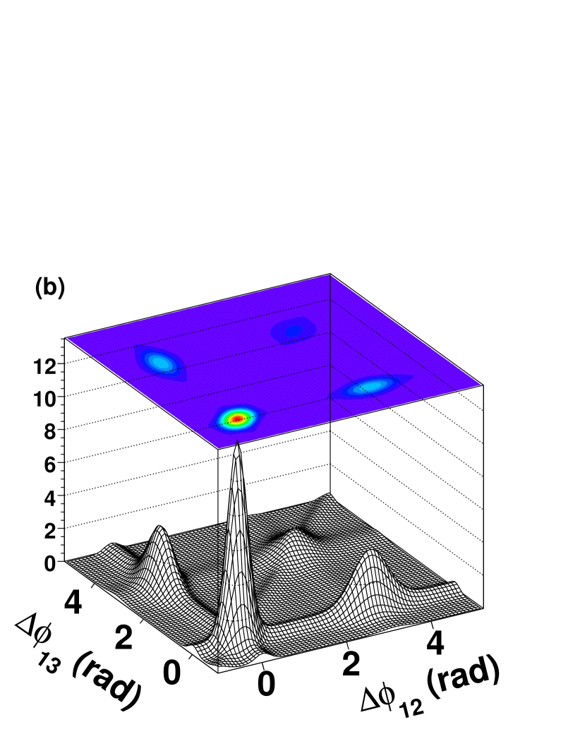
Figure 1: 3-Cumulants calculated based on the Gaussian jet model discussed in the text. (a) Poisson case, (b) Non-Poisson case with $\langle J(J-1)\rangle-\langle J\rangle^{2}=0.05\langle J\rangle$

III.2 Collective Flow

Flow, or collective motion, is an important feature of heavy ion collisions at relativistic energies. It manifests itself by a modification of transverse momentum ($p_{t}$) spectra relative to those observed in $p+p$ collisions, and by azimuthal anisotropy of produced particles. In this section, we focus on azimuthal anisotropy arising in non-central heavy ion collisions. We decompose the azimuthal anisotropy in terms of harmonics relative to an assumed reaction plane. The conditional probability, $P_{F}(\varphi_{i}|\psi)$, to observe a particle at a given azimuthal angle, $\varphi_{i}$, with the reaction plane at angle, $\psi$, is written as a Fourier series.

$$P_{F}(\varphi_{i}|\psi)=F_{2}(\varphi_{i}-\psi;v_{m}(i)).$$ (18)

where

$$F_{2}(\Delta\varphi;v_{m})=1+2\sum\limits_{m}{v_{m}}\cos\left({m\left({\Delta\varphi}\right)}\right)$$ (19)

The Fourier coefficients $v_{m}(i)$ measure the m-th order anisotropy for particles emitted in a selected kinematic range $i$. Measurements have shown the second order (elliptical) anisotropy can be rather large in $Au+Au$ collisions at RHIC while first and fourth order harmonics are typically much smaller. STAR measurements show the fourth harmonic scales roughly as the square of the second order harmonic ($v_{4}\approx 1.1v_{2}^{2}$) WhitePapers ; StarV4 . The third and fifth harmonics are by symmetry null at $\eta=0$ for a colliding system such as $Au+Au$, and expected to be rather small at other rapidities. Higher harmonics are most likely negligible. We neglect possible event-to-event fluctuations of these coefficients given it emerges from recent works disentangling flow fluctuations and non-flow correlations is difficult. We describe the probability of finding $N_{i}$ particles in the kinematical range $i$ according to probability $P(N_{i})$. The exact form of this probability is not required. Only its first, second, and third moments are needed. The joint probability of measuring $N_{i}$ particles at an angle $\varphi_{i}$ while the reaction plane angle is at $\psi$ is given by $P_{F}(\varphi_{i},N_{i},\psi)=P_{F}(\varphi_{i}|\psi)P_{F}(N_{i})P_{RP}(\psi)$ where $P_{RP}(\psi)=(2\pi)^{-1}$ is the probability of finding the reaction plane at a given angle $\psi$. Integration yields the single particle density $\rho_{1}(\varphi_{i})=\left({2\pi}\right)^{-1}\left\langle{N_{i}}\right\rangle$. The flow 2- and 3-cumulants are given respectively by (see Ref.Pruneau06 for a derivation of these expressions):

$$C_{2}^{F}(\Delta\varphi_{ij}) = \left(2\pi\right)^{-2}\left(\left\langle N_{i}N_{j}\right\rangle F_{2}(\Delta\varphi_{ij};v_{m}(i)v_{m}(j))-\left\langle N_{i}\right\rangle\left\langle N_{j}\right\rangle\right)$$

$$= \left(2\pi\right)^{-2}\left\langle N_{i}N_{j}\right\rangle$$

$$\times\left({1-d_{ij}+2\sum\limits_{m}{v_{m}(i)v_{m}(j)\cos\left({m\Delta\varphi_{ij}}\right)}}\right)$$

and

$$C_{3}^{F}(\varphi_{i},\varphi_{j},\varphi_{k}) = (2\pi)^{-3}\left\langle N_{1}N_{2}N_{3}\right\rangle\left[\Phi_{3}(\varphi_{i},\varphi_{j},\varphi_{k})\right.$$

$$+ \left(1-f_{ijk}\right)\Phi_{2}(\Delta\varphi_{ij})$$

$$+ \left(1-f_{ikj}\right)\Phi_{2}(\Delta\varphi_{ik})$$

$$+ \left(1-f_{jki}\right)\Phi_{2}(\Delta\varphi_{jk})$$

$$+ \left.1-f_{ijk}-f_{ikj}-f_{jki}+2g_{ijk}\right]$$

where

$$\Phi_{2}(x;v_{1,m},v_{2,m})=2\sum\limits_{m=1}^{\infty}{v_{1,m}v_{2,m}\cos(mx)}$$ (22)

and

$$\Phi_{3}(\varphi_{i},\varphi_{j},\varphi_{k})=2\sum\limits_{p,m,n}{v_{1,p}v_{2,m}v_{3,n}\left[\begin{array}[]{l}\delta_{p,m+n}\cos\left({p\varphi_{i}-m\varphi_{j}-n\varphi_{k}}\right)\\ +\delta_{m,p+n}\cos\left({-p\varphi_{i}+m\varphi_{j}-n\varphi_{k}}\right)\\ +\delta_{n,m+p}\cos\left({-p\varphi_{i}-m\varphi_{j}+n\varphi_{k}}\right)\\ \end{array}\right]}$$ (26)

$v_{i,m}$ correspond to the anisotropy coefficients of order $m$ for particle $i$. The coefficients $d_{ij}$, $f_{ijk}$, and $g_{ijk}$ are defined as follows

$$d_{ij} = \frac{{\left\langle{N_{i}}\right\rangle\left\langle{N_{j}}\right\rangle}}{{\left\langle{N_{i}N_{j}}\right\rangle}}$$

$$f_{ijk} = \frac{{\left\langle{N_{i}N_{j}}\right\rangle\left\langle{N_{k}}\right\rangle}}{{\left\langle{N_{i}N_{j}N_{k}}\right\rangle}}$$ (27)

$$g_{ijk} = \frac{{\left\langle{N_{i}}\right\rangle\left\langle{N_{j}}\right\rangle\left\langle{N_{k}}\right\rangle}}{{\left\langle{N_{i}N_{j}N_{k}}\right\rangle}}$$

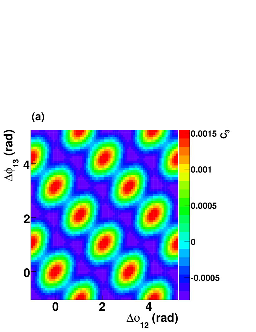
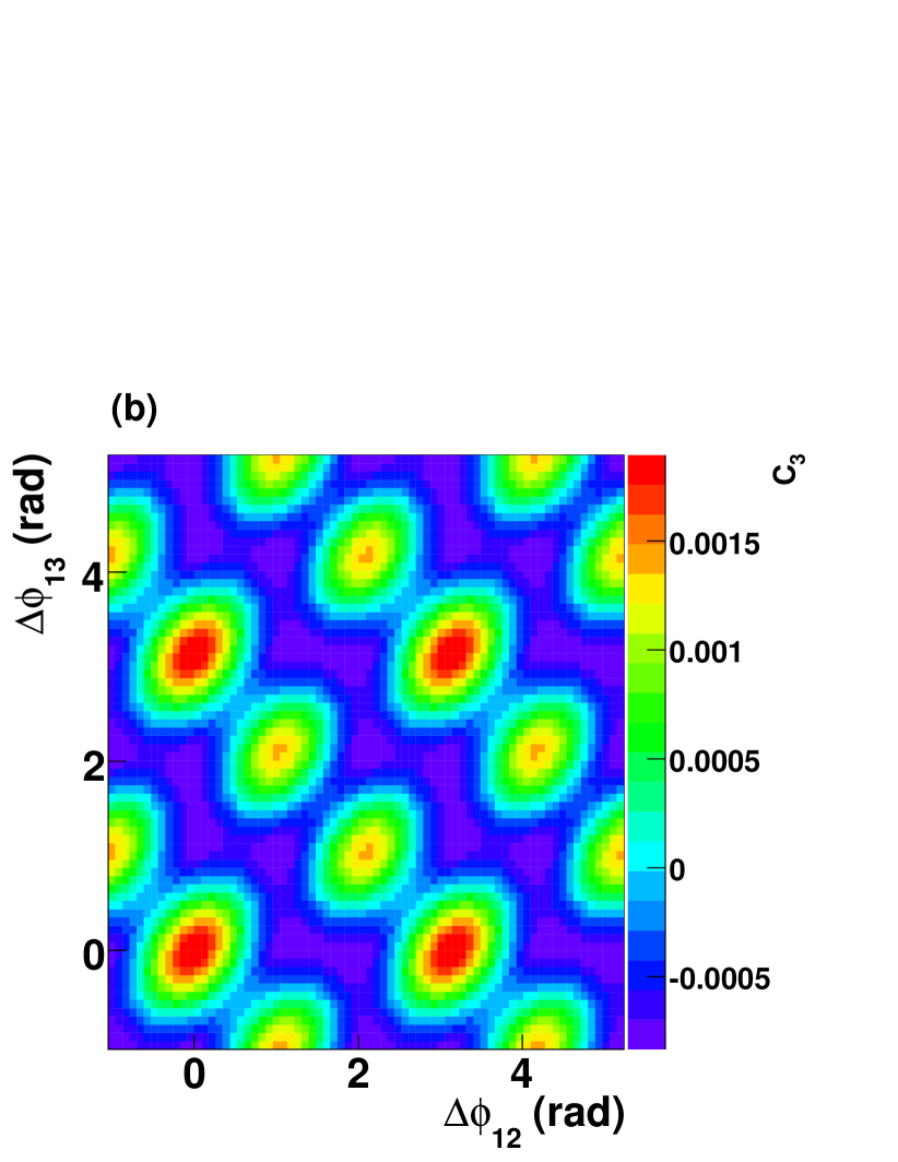
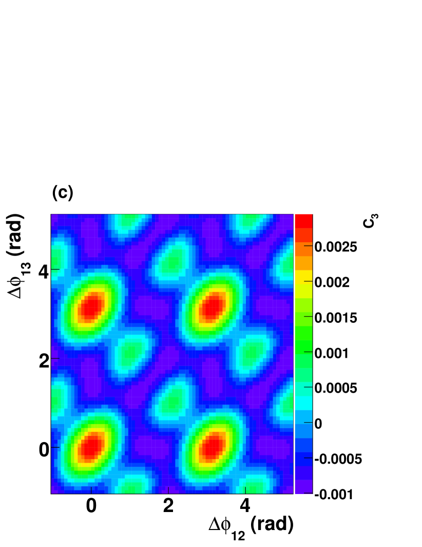
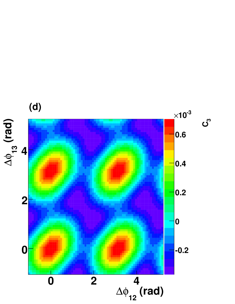
Figure 2: 3-cumulant flow signal calculated using (a) only $v_{2}v_{2}v_{4}$ terms, (b) $v_{2}v_{2}v_{4}$ and $v_{2}v_{2}+v_{4}v_{4}$ terms in 1:0.5 ratio, (c) $v_{2}v_{2}v_{4}$ and $v_{2}v_{2}+v_{4}v_{4}$ terms in a 1:2 ratio, (d) only $v_{2}v_{2}+v_{4}v_{4}$ terms. The $v_{2}v_{2}v_{4}$ and $v_{2}v_{2}+v_{4}v_{4}$ terms are calculated according to Eqs. III.2-III.2. See text for details.

We find that the flow 3-cumulant involves, in general, an arbitrary combination of second (e.g. $v_{2}^{2}$) and third order (e.g. $v_{2}v_{2}v_{4}$) terms. If particle production is strictly Poissonian, the coefficients $f_{ijk}$ and $g_{ijk}$ are unity. The second order terms of the cumulant thus vanish, and the 3-cumulant (flow only) then reduces to:

$$C_{3}^{F,Poisson}(\varphi_{1},\varphi_{2},\varphi_{3})=\left({2\pi}\right)^{-3}\left\langle{N_{1}N_{2}N_{3}}\right\rangle\Phi_{3}(\varphi_{1},\varphi_{2},\varphi_{3};v_{p}(1)v_{m}(2)v_{n}(3))$$ (28)

which features only non-diagonal terms $v_{m}(i)v_{n}(j)v_{p}(k)$, i.e. with $m\neq n$, $m\neq p$, or $n\neq p$. This is illustrated in Figure 2 (a) which shows the flow 3-cumulant calculated using only $v_{2}v_{2}v_{4}$ terms. In general, particle production is non-Poissonian, and second order terms must be considered. The flow 3-cumulant shown in Fig. 2 (b) and (c) includes $v_{2}^{2}$ and $v_{4}^{2}$ added in ratios 1:0.5, and 1:2 respectively to the $v_{2}v_{2}v_{4}$ terms. Only $v_{2}^{2}$ and $v_{4}^{2}$ terms are included in Fig 2 (d) illustrating a case where non-Poisson fluctuations are very large, and thereby dominate the 3-cumulant. The shape of the 3-cumulant thus depends significantly on the strength of the non-Poisson (2^nd order terms), as well as the magnitude of the flow coefficients. The interpretation of measured 3-cumulants may thus be considerably complicated by the presence of non-Poisson fluctuations.

Experimentally, one can estimate the magnitude of second order (diagonal) terms from measured total numbers of triplet, pair, and single particle densities. STAR observes based on data from Au + Au collisions at 200 GeV StarC308 , the coefficients $f_{123}$ and $f_{231}$ deviate from unity. The size of the deviation scales qualitatively as the inverse of the event multiplicity. STAR also finds the magnitude of the deviation depends on the specific particle kinematic ranges used to carry the analysis. The particle production process is manifestly non-Poissonian. Since the bulk of produced particles exhibits elliptic flow, this implies the conditions $f_{ijk}=g_{ijk}=1$ are not verified in practice. The second order and constant terms of the cumulant do not vanish, and may in fact be sizable. The 2^nd second order terms result from number fluctuations, and may in principle be estimated (and thus fitted) on the basis of measurements of $f_{ijk}$. Note however that multiplicity fluctuations occur for flow-like processes as well as all other types of production processes (including jets, conical emission, etc). It is thus non-trivial to unambiguously evaluate the proper magnitude of the diagonal flow terms based on ratios of measured yields.

Effects of flow fluctuations are not specifically addressed in the above flow model. Note however that, as defined, the 3-cumulant measures averages of $\langle v_{n}^{2}\rangle$, and $\langle v_{i}v_{j}v_{k}\rangle$ coefficients rather than averages of $\langle v_{n}\rangle$. The 3-cumulant thus implicitely features fluctuations and non-flow effects. Given it is difficult to experimentally distinguish flow fluctuations and non-flow effects (see for instance the review by Voloshin et al. VoloshinReview08 ), analyses attempting explicit subtraction of flow contributions (from three particle densities) based on the above equations, are thus intrinsically non-robust.

III.3 Conical Emission

Mach cone emission of particles by partons propagating through dense QGP matter was proposed by Stoecker Stoecker05 to explain the peculiar dip structure found at $180^{o}$ in two-particle correlations reported by the STAR and PHENIX collaborations, and is the subject of many recent theoretical investigations Stoecker76 ; Stoecker05 ; JRuppert05 ; RupperMuller05 ; SolanaShuryak05 ; RenkRuppert06 ; Heinz06 ; Stocker07 ; RenkRupper07 ; MullerQM08 ; BBetz08 ; Armesto04 ; Salgado05a ; RenkRuppert07_PLB646 ; Voloshin05 ; Hwa05_PRC74 . The concept of Mach cone emission is based on the notion that high momentum partons propagating through a dense QGP interact with the medium and loose energy (and momentum) at a finite rate. The release of energy engenders a wake that propagates at a characteristic angle, the Mach angle, determined by the sound velocity in the medium. Authors of Ref. SolanaShuryak05 estimated the speed of sound in the QGP to be of the order of $v_{s}\approx c_{s}^{RHIC}\approx 0.33$. The Mach angle should thus be of the order of $70^{o}$ relative to the away-side parton direction. We use this prediction to motivate a simple geometrical model of conical emission. The near- side jet is described using a Gaussian azimuthal profile. Away side particles are emitted at a cone angle of 1 radian with a scatter of 0.05 radian relative to the away-side direction. Figures 7 (a-b) present the 3-cumulant obtained with a Monte Carlo simulation based on two million events. Given that Mach cone particles are produced at 1 radian from the away-side direction and roughly normal to the beam direction, narrow Jacobian peaks are seen in the three-particle correlations. A strong dip is present at $180^{o}$ in the two-particle correlations, while in the three-particle correlation a clear spacing is found between the peaks. In this simple model,the finite width of the peaks is due in part to the finite width of the trigger jet, and in part to the scatter imparted to the cone particles relative to the away-side direction. In practice, one might expect additional broadening of the cone because the speed of sound changes through the life of the QGP medium, and given the finite size of the medium. Radial flow might also significantly alter the correlation functions. As discussed in Pruneau06 , the details of the correlation shapes clearly depend on assumptions made about the kinematics of the away-side parton.

III.4 Flow $\times$ Jet Correlations

The measured nuclear modification factor, $R_{AA}$, defined as the ratio single particle yields measured in $A+A$ collision to those measured in $p+p$ interactions (scaled by the number of binary collisions in $A+A$) suggest the propagation of jets through the medium is severely quenched, and therefore features a surface emission bias WhitePapers . In this scenario, partons propagating through the medium loose a large fraction of their energy. This results into jet lost or lower energy jets with smaller particle multiplicity. The path length through the medium determines the amount of energy loss and quenching. At a given point of emission, near the medium surface, a parton propagating outward in a direction normal to the surface should have shortest pathway through the medium, and minimal energy loss. Partons produced at the same location, but emitted in other directions would have longer path through the medium and suffer larger energy loss. In this scenario, one thus expects jet yields (and consequently the high $p_{t}$ trigger) to be correlated to the reaction plane orientation. Neglecting disturbances imparted to the medium by the propagation of the jet (or parton), we model the jet dependency on azimuthal angle relative to the reaction plane with Fourier decomposition. Specifically, we write the probability of the jet being emitted at angle $\phi$ while the reaction plane is at angle $\psi$ as

$$P(\phi|\psi)=1+2\sum\limits_{n}{a_{n}\cos}\left({n(\phi-\psi)}\right)$$ (29)

where the coefficients $a_{n}$ represent the effect of the differential azimuthal attenuation. We parameterize the jet multiplicity and azimuthal width using associated yields, and Gaussian widths that do not depend on the azimuthal direction. As in Sec. III.1, the average number of jets per event is written $\left\langle J\right\rangle$ while the number of particles associated with a given jet is $\left\langle{A_{i}}\right\rangle$. We also assume the presence of a flowing background consisting on average of $\left\langle{B_{i}}\right\rangle$ particles. The single particle yield is thus $\rho_{1,J\otimes F}(\varphi_{i})=(2\pi)^{-1}\left({\left\langle J\right\rangle\left\langle A_{i}\right\rangle+\left\langle B_{i}\right\rangle}\right)$. Given the production of both jets, and background particles is correlated to the reaction plane, one ends up with flow-induced correlations between all particles, even those produced by the jets. The two-particle cumulant involves three sets of terms, namely jet-jet ($J\otimes J$), jet-background ($J\otimes B$), and background-background ($B\otimes B$). Similarly, the three-particle cumulant involves $J\otimes J\otimes J$, $J\otimes J\otimes B$, $J\otimes B\otimes B$, and $B\otimes B\otimes B$ terms.

A jet-flow model was already discussed in Pruneau06 . We here re-derive, and express the various terms of the model with a more compact and intuitive notation. The terms, $B\otimes B$ and $B\otimes B\otimes B$ are identical in form to those considered in Sect III.2. We need to discuss only the terms $J\otimes J$, $J\otimes B$, $J\otimes J\otimes J$, $J\otimes J\otimes B$, and $J\otimes B\otimes B$. We begin with $J\otimes J$, and $J\otimes J\otimes J$. These terms contain contributions where two (three) of the particles are part of the same jet, and others where one, or two particles are not from the same jet. When particles are from the same jet, the correlation to the reaction plane is unimportant (to the extent, in our model, that the width of the jets do not change with their orientation relative to the reaction plane). The corresponding terms are thus identical to those obtained in the absence of flow. The two-particle density includes a term with two particles from the same jet (identical to that discussed in Sec. III.1), and a term with particles from two different jets. This last term is given by:

$$\left\langle{J(J-1)}\right\rangle\left\langle{A_{i}}\right\rangle\left\langle{A_{j}}\right\rangle\int{d\psi d\phi_{\alpha}G(\varphi_{i}-\phi_{\alpha})}$$ (30)

$$\times P(\phi_{\alpha}|\psi)\int{d\phi_{\beta}G(\varphi_{i}-\phi_{\beta})P(\phi_{\beta}|\psi)}$$

Integration, and inclusion of the first term yields the jet component of the two-particle density.

$$\rho_{2}^{Jetonly}(\varphi_{i},\varphi_{j}) = \left\langle J\right\rangle\left\langle{A_{i}A_{j}}\right\rangle G_{2}(\varphi_{i}-\varphi_{j};\sigma_{12})$$

$$+\left\langle{J(J-1)}\right\rangle\left\langle{A_{i}}\right\rangle\left\langle{A_{j}}\right\rangle F_{2}(\varphi_{i}-\varphi_{j};a_{n}(i,j))$$

where $\sigma_{12}^{2}=\sigma_{1}^{2}+\sigma_{2}^{2}$, $a_{n}(i,j)=v_{n}^{\prime}(i)v_{n}^{\prime}(j)$, with $v_{n}^{\prime}(i)=a_{n}\exp(-n^{2}\sigma_{i}^{2}/2)$. Similarly, the three-particle density includes a term with three particle from the same jet, two particles from the same jet, and another with all three particles from different jets. The $J\otimes J$, and $J\otimes J\otimes J$ part og the cumulant is as follows.

$$\rho_{3}^{Jetonly}(\varphi_{i},\varphi_{j},\varphi_{k}) = \left\langle J\right\rangle\left\langle{A_{i}A_{j}A_{k}}\right\rangle G_{3}(\varphi_{i},\varphi_{j},\varphi_{k};\sigma_{i},\sigma_{j},\sigma_{k})$$

$$+\left\langle J(J-1)\right\rangle\left\langle A_{i}A_{j}\right\rangle\left\langle A_{k}\right\rangle G_{2}(\Delta\varphi_{ij})F_{2}\left({\frac{\sigma_{j}^{2}}{\sigma_{ij}^{2}}\varphi_{i}+\frac{\sigma_{i}^{2}}{\sigma_{ij}^{2}}\varphi_{j}-\varphi_{k};v_{n}^{\prime\prime}(k)}\right)+(jki)$$

$$+\left\langle J(J-1)(J-2)\right\rangle\left\langle A_{i}\right\rangle\left\langle A_{j}\right\rangle\left\langle A_{k}\right\rangle N_{3}(\varphi_{i},\varphi_{j},\varphi_{k};v_{n}^{\prime}(i),v_{m}^{\prime}(j),v_{p}^{\prime}(k))$$

The functions $G_{3}$, $F_{3}$, $F_{2}$ were defined in previous sections. The symbol $(jki)$ indicates identical terms obtained by permutation of the indices. The term $G_{3}$ is identical to that obtained for non-flowing jets. The term of the last row corresponds to a flow-like correlation between the three measured particles, albeit with a strength which depends on the fluctuations of the number of jets per event, and the jet associated multiplicities in the kinematic ranges considered. The second row contains three similar terms that embody the jet-flow correlations: two particles are correlated because they belong to the same jet, while the third is correlated to the first two because of reaction plane dependencies. One notes that in the above expression, $F_{2}$ depends on the angle of emission of all three particles (at variance with assumptions made in Ref. Ulery06a ; Ulery06b ) in a non trivial way. Indeed, in general, the jet correlation widths $\sigma_{i}$ depend on the particle momentum ranges: the ratios ${{\sigma_{i}^{2}}\mathord{\left/{\vphantom{{\sigma_{i}^{2}}{\sigma_{ij}^{2}}}}\right.\kern-1.2pt}{\sigma_{ij}^{2}}}$ are arbitrary (non-integer) values. $F_{2}$ therefore involves inharmonic flow components. This implies it is inappropriate to model jet-flow cross-terms as a simple product of jet-like correlations, and flow-like correlations, as in Ref. Ulery06a ; Ulery06b , for purposes of background subtraction.

We next consider the component $J\otimes J\otimes B$, and $J\otimes B\otimes B$ of the 3-cumulant. Following the steps used for the derivation of the pure jet components, one finds it also includes a term proportional to $F_{2}G_{2}$ indistinguishable from $J\otimes J\otimes J$. One has

$$\left\langle J\right\rangle\left\langle{A_{1}A_{2}}\right\rangle\left\langle{B_{3}}\right\rangle G_{2}(\Delta\varphi_{12};\sigma_{12})F\left({\frac{{\sigma_{2}^{2}}}{{\sigma_{12}^{2}}}\varphi_{1}+\frac{{\sigma_{1}^{2}}}{{\sigma_{12}^{2}}}\varphi_{2}-\varphi_{3};v_{n}^{\prime\prime}(3)}\right)$$ (33)

The $J\otimes B\otimes B$ compoment of the 3-cumulant contains a non-diagonal flow term as follows

$$\left\langle J\right\rangle\left\langle{A_{1}}\right\rangle\left\langle{B_{2}B_{3}}\right\rangle F_{3}(\varphi_{i},\varphi_{j},\varphi_{k};v_{n}^{\prime}(i),v_{m}^{\prime}(j),v_{p}^{\prime}(k))$$ (34)

This term has the same functional dependence and is indisguishable from the term on the third line of Eq III.4. Assemblinging all components, one obtains the JET $\otimes$ FLOW 3-cumulant:

$$C_{3}^{J\otimes F}(\varphi_{i},\varphi_{j},\varphi_{k}) = \left\langle J\right\rangle\left\langle{A_{i}A_{j}A_{k}}\right\rangle G_{3}(\varphi_{i},\varphi_{j},\varphi_{k};\sigma_{i},\sigma_{j},\sigma_{k})$$

$$+ \left({\left\langle{J(J-1)}\right\rangle-\left\langle J\right\rangle^{2}}\right)\left\langle{A_{i}A_{j}}\right\rangle\left\langle{A_{k}}\right\rangle G_{2}(\Delta\varphi_{ij})+(jki)$$

$$+ \left\langle{A_{i}A_{j}}\right\rangle\left({\left\langle{J(J-1)}\right\rangle\left\langle{A_{k}}\right\rangle+\left\langle J\right\rangle\left\langle{B_{k}}\right\rangle}\right)G(\Delta\varphi_{ij};\sigma_{ij})\Phi_{2}\left({\frac{{\sigma_{j}^{2}}}{{\sigma_{ij}^{2}}}\varphi_{i}-\frac{{\sigma_{i}^{2}}}{{\sigma_{ij}^{2}}}\varphi_{j}-\varphi_{k};v_{n}^{\prime\prime}(k)}\right)+(jki)$$

$$- \left\langle{J(J-1)}\right\rangle\left\langle{A_{i}}\right\rangle\left\langle{A_{j}}\right\rangle\left\langle{A_{k}}\right\rangle F_{2}(\varphi_{i}-\varphi_{j};a_{n}(i,j))+(jki)$$

$$+ \left\langle{J(J-1)(J-2)}\right\rangle\left\langle{A_{i}}\right\rangle\left\langle{A_{j}}\right\rangle\left\langle{A_{k}}\right\rangle N_{3}(\varphi_{i},\varphi_{j},\varphi_{k};v_{n}^{\prime}(i),v_{m}^{\prime}(j),v_{p}^{\prime}(k)$$

$$+ \left\langle J\right\rangle\left\langle{A_{i}}\right\rangle\left\langle{B_{j}B_{k}}\right\rangle N_{3}(\varphi_{i},\varphi_{j},\varphi_{k};v_{n}^{\prime}(i),v_{m}^{\prime}(j),v_{p}^{\prime}(k))$$

$$- \left\langle{B_{i}B_{j}}\right\rangle\left\langle J\right\rangle\left\langle{A_{k}}\right\rangle F_{2}\left({\varphi_{i}-\varphi_{j};v_{n}(i)v_{n}(j)}\right)+(jki)$$

$$+ \left({2\pi}\right)^{-3}\left\langle{B_{i}B_{j}B_{k}}\right\rangle\Phi_{3}(\varphi_{i},\varphi_{j},\varphi_{k};v_{p}(i)v_{m}(j)v_{n}(k)_{k})$$

$$+ \left({2\pi}\right)^{-3}\left\langle{B_{i}B_{j}B_{k}}\right\rangle\left({1-f_{ijk}}\right)\Phi_{2}(\varphi_{i}-\varphi_{j};v_{m}(i),v_{m}(j))+(jki)$$

$$- \left({2\pi}\right)^{-3}\left\langle{B_{i}B_{j}B_{k}}\right\rangle f_{ijk}+(jki)$$

$$+ constants$$ (36)

This cumulant includes components typical of jets (line 1 and 2), flow (line 4-11’), and one term unique to jet-flow cross-term (line 3). While this jet-flow term does include two-particle jet-like, and flow-like factors, it is important to note the flow factor is intrinsically inharmonic. Its amplitude depends on the number jet associates and background particle multiplicity. Given the number of associates is likely much smaller than the number of background particles, one expects the amplitude of this term to be dominated by the magnitude of the background. It is interesting to compare the magnitude of this cross-term relative to the off-diagonal flow terms. We focus on the difference between the leading terms in $v_{2}v_{2}v_{4}$ and $v_{2}v_{2}$. Given the jet cross section and fragment multiplicity are small at RHIC energies, one expects the $v_{2}v_{2}v_{4}$ term should dominate or at most be of similar magnitude to the cross-term unless the jet flow $v_{2}$ is considerably larger than the bulk flow.

As discussed in Sect III.2, particle emission in $A+A$ collisions is a non-Poissonian process. The coefficients $f_{ijk}$ in general deviate from unity. The leading background terms may thus be those of line 2, 6, 7, and 9 in Eq. 36.

Lines 4 and 7 both contain terms in $F_{2}$ albeit with different amplitudes. Experimentally these cannot be distinguished, and one ends up with an $F_{2}$ contribution to the cumulant which depends on both the jet and background yields. Likewise, lines 5, 6, 8, and 9 feature non-diagonal flow terms (dominated by $v_{2}v_{2}v_{4}$) which cannot be distinguished experimentally: the amplitude of the $v_{2}v_{2}v_{4}$ three particle correlation terms depend intricately on the jet yield, its fluctuations, as well as the background yield. The jet-flow ’cross-term’ manifests itself through the inharmonic terms of line 3 in Eq. 36. While these harmonic terms may be approximated as a product such as $G_{2}(\Delta\phi_{12})F\Phi_{2}(\Delta\phi_{13})$ if the width $\sigma_{1}$ (very high-$p_{t}$ particles) is negligible, when added in quadrature, to the width $\sigma_{2}$ of the low-$p_{t}$ particle, the approximation breaks down in general because $\sigma_{1}$ is neither zero or equal to $\sigma_{2}$. Additionally, note that the model used in this section assumed the cross-terms are dominated by jetty and flow components. This may not be the case in practice. For instance resonance or cluster decays in the presence of both radial and elliptical flow should lead to complex cross terms. Such cross-terms shall be inhenrently inharmonic also. Given the correlation shapes associated with resonance or cluster decays can be quite wide, the inharmonic character of the cross term can be quite intricate. Adhoc subtraction of terms in $G_{2}(\Delta\phi_{12})F\Phi_{2}(\Delta\phi_{13})$ in model based analyses is therefore unwarranted.

IV Probability Cumulants

We showed in Section III.2 that the 3-cumulant associated with flow reduces to non- diagonal terms in $v_{n}v_{m}v_{p}$ for Poissonian particle production processes. However, momentum, energy, and quantum number conservation laws imply elementary collisions are typically non-Poissonian processes as observed from Fig 3 which shows ratios $f_{ijk}$ measured by STAR StarC308 . This implies the 3-cumulant may have a rather complicated structure, with second order terms (i.e. two-particles) as well as three particle terms. We note however that the simplicity of the 3-cumulant may be recovered, in this case, by using probability cumulants rather than density cumulants. The probability cumulants are defined as follows:

$$P_{2}(\varphi_{i},\varphi_{j}) \equiv \frac{{\rho_{2}(\varphi_{i},\varphi_{j})}}{{\left\langle{N_{i}N_{j}}\right\rangle}}-\frac{{\rho_{1}(\varphi_{i})\rho_{1}(\varphi_{j})}}{{\left\langle{N_{i}}\right\rangle\left\langle{N_{j}}\right\rangle}}$$ (37)

$$P_{3}(\varphi_{i},\varphi_{j},\varphi_{k}) \equiv \frac{{\rho_{3}(\varphi_{i},\varphi_{j},\varphi_{k})}}{{\left\langle{N_{i}N_{j}N_{k}}\right\rangle}}-\frac{{\rho_{2}(\varphi_{i},\varphi_{j})\rho_{1}(\varphi_{k})}}{{\left\langle{N_{i}N_{j}}\right\rangle\left\langle{N_{k}}\right\rangle}}$$

$$- \frac{{\rho_{2}(\varphi_{i},\varphi_{k})\rho_{1}(\varphi_{j})}}{{\left\langle{N_{i}N_{k}}\right\rangle\left\langle{N_{j}}\right\rangle}}-\frac{{\rho_{2}(\varphi_{j},\varphi_{k})\rho_{1}(\varphi_{i})}}{{\left\langle{N_{j}N_{k}}\right\rangle\left\langle{N_{i}}\right\rangle}}$$

$$+ 2\frac{{\rho_{1}(\varphi_{i})\rho_{1}(\varphi_{j})\rho_{1}(\varphi_{k})}}{{\left\langle{N_{i}}\right\rangle\left\langle{N_{j}}\right\rangle\left\langle{N_{k}}\right\rangle}}$$

where $N_{i}$ correspond to total particle multiplicities accepted in the kinematic cuts $i$. It is straightforward to verify that the flow probability 3-cumulant indeed consists of non-diagonal flow terms only:

$$P^{N}_{3}(\varphi_{1},\varphi_{2},\varphi_{3})=\left({2\pi}\right)^{-3}\Phi_{3}(\varphi_{1},\varphi_{2},\varphi_{3};v_{p}(1)v_{m}(2)v_{n}(3))$$ (39)

The probability cumulant, $P_{3}$, thus provides a tool to suppress the strength of non-Poissonian 2^nd order terms, and may therefore be used, in addition to the number 3-cumulant, $C_{3}$, in three-particle analyses.

The simplification obtained for flow processes is unfortunately not realized for jet or conical emission processes. The use of probability 3-cumulant may then be of limited interest in practice. This can be straightforwardly shown through a calculation of the probability cumulant of the Gaussian model used in Sec. III.1. We limit our calculation to the near side jet. One finds the probability 3-cumulant contains terms in $G_{2}(\Delta\phi)$ proportional to the non vanishing factor $\left\langle{J(J-1)}\right\rangle\left\langle{N_{1}N_{2}}\right\rangle\left\langle{N_{3}}\right\rangle-\left\langle J\right\rangle^{2}\left\langle{N_{1}N_{2}N_{3}}\right\rangle$, where ${N_{1}}$, ${N_{1}N_{2}}$, and ${N_{1}N_{2}N_{3}}$ are respectively the number of singles, pairs, and triplets from the near side jet. By contrast to the flow probability 3-cumulant which contains only genuine three-particle correlation terms ($\Phi_{3}$), the Gaussian probability cumulant thus has a complicated expression which contains terms in $G_{3}$ as well as in $G_{2}$. Its interpretation is therefore non trivial.

V Efficiency Correction and Observable Robustness

Measured particle densities, and cumulants must be corrected for detection efficiencies and other instrumental effects. We introduced in Ref. Pruneau06 a procedure to correct for detector efficiencies based on ratios of two- and three-particle densities by products of two, and three single particle densities. For instance, up to a global efficiency factor, the corrected three-particle density is given by

$$\rho_{3}(\varphi_{1},\varphi_{2},\varphi_{3})_{corrected}=\left({2\pi}\right)^{-3}N(1)N(2)N(3)\frac{{N_{3}(\varphi_{1},\varphi_{2},\varphi_{3})}}{{N_{1}(\varphi_{1})N_{1}(\varphi_{2})N_{1}(\varphi_{3})}}$$ (40)

where $N_{1}(\varphi_{i})$ stands for uncorrected single particle densities, $N_{3}(\varphi_{1},\varphi_{2},\varphi_{3})$ are numbers of triplets, and $N(i)$ are total particle yields within the kinematics cuts $i$.

This correction procedure is strictly exact for continuous functions provided the efficiency is a function of the azimuthal angles $\varphi_{i}$ but independent of other observables such as the particle rapidity and transverse momentum. For large detectors such as the STAR TPC StarNim , the efficiency is a smooth and slowly varying function of the pseudorapidity and transverse momentum, but exhibit periodic structures in azimuth because of TPC sector boundaries. A correction for azimuthal dependencies of the detector response is thus the most important and relevant in this context.

We examine the robustness of the above correction procedure in a practical situation, i.e. where the densities are measured with a finite number of bins, based on the jet and conical emission models discussed in Sec. 2. We parameterize the detection efficiency, $\varepsilon(\varphi_{i})$, with a Fourier decomposition.

$$\varepsilon(\varphi_{i})=\varepsilon_{0}\left({1+2\sum\limits_{n=1}^{\infty}{\varepsilon_{i}\cos\left({n\varphi_{i}}\right)}}\right)$$ (41)

where $\varepsilon_{0}$ is the average efficiency, and coefficients $\varepsilon_{n}$ determine the azimuthal dependence of the efficiency. We assume the efficiency for simultaneously detecting two and three particles are factorizable as product of single particle efficiencies. The mean single particle detection efficiency is set to 80%. The Fourier coefficients (Eq. 41) are chosen to obtain a non-uniform azimuthal detector response as shown in Fig. 3.

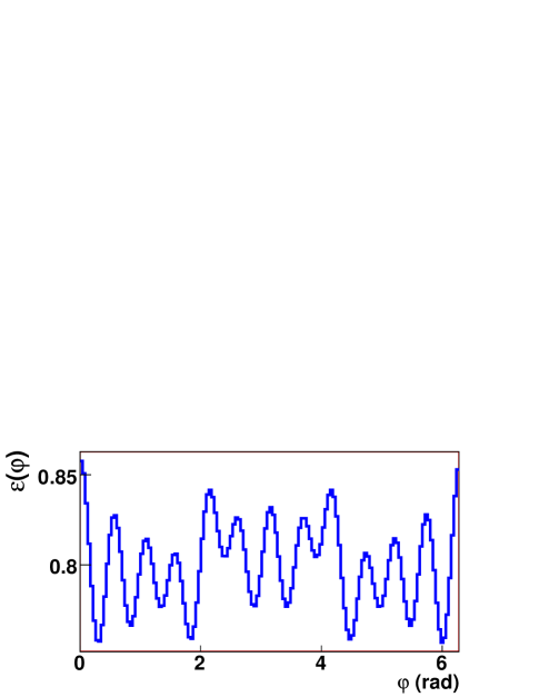
Figure 3: (Color online) Detection efficiency dependence on the particle azimuthal angle used in the simulation results presented in Fig. 4.

The JET+Mach Cone model described in sections III.3 and VI is used to carry a simulation of the robustness of the correction procedure. Figure 4 (a) displays the 3-cumulants obtain with perfect detection efficiency. Figure 4 (b) shows the uncorrected two particle density $\rho_{2}(\varphi_{1},\varphi_{2})$ obtained with the non-uniform azimuthal response illustrated in Fig 3. The two particle density exhibits strong, narrow, and repeated structures that result from the twelve-fold structure of the assumed detector response. Figure 4 (c) displays the 3-cumulant obtained with the same detector response, but corrected for efficiency effects by division of the two and three particle densities by the product of single particle densities, as in Eq. 40. In stark contrast to the correlation shown in Figure 4 (b), one finds the corrected cumulant exhibits no evidence of the detector response except for a global change in amplitude corresponding to the cube of the average detection efficiency. Figure 4 (d) shows the difference between this cumulant and the perfect efficiency cumulant scaled down by the cube of the average detection efficiency. The standard deviation of the difference is smaller than 1% of the maximum 3-cumulant amplitude and exhibit no particular structure. We thus conclude the correction method is numerically robust for cases where the triplet, and pair efficiencies factorize.

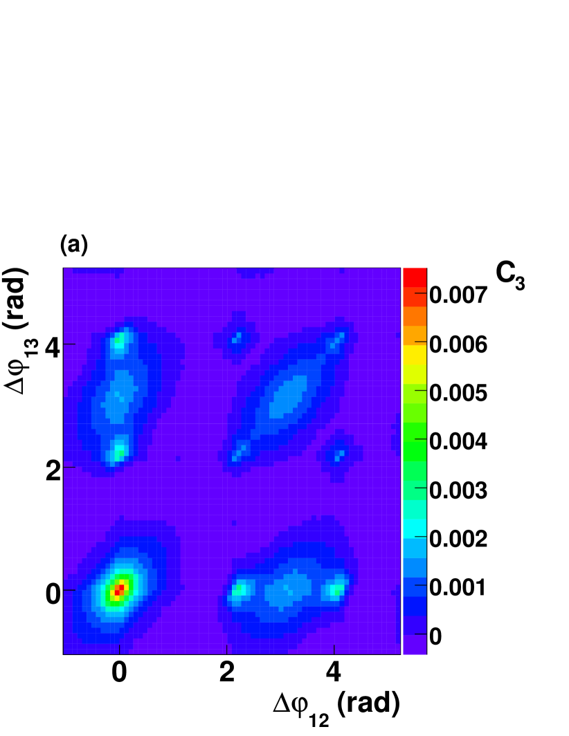
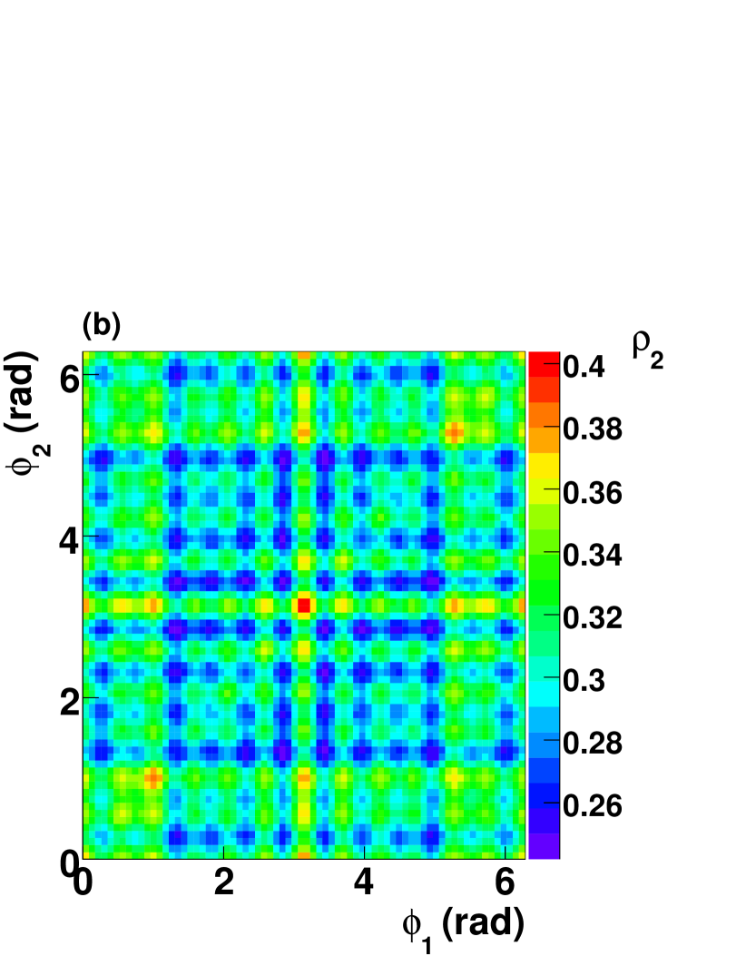
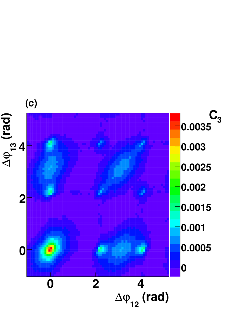
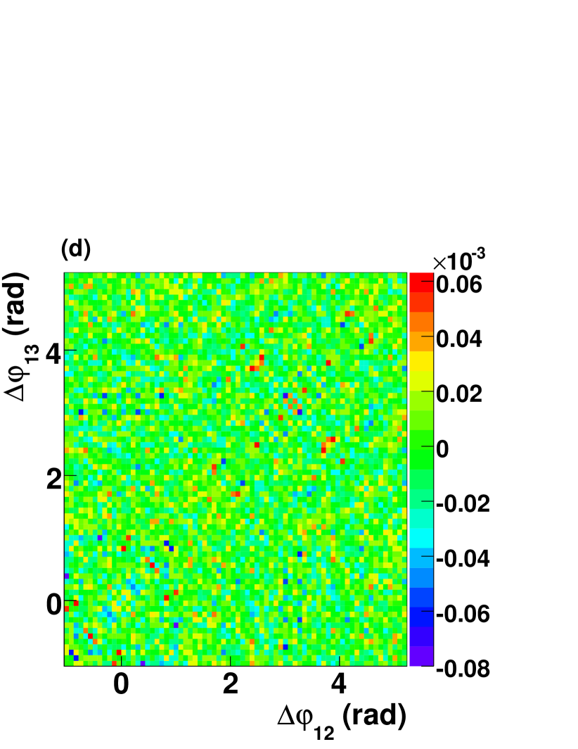
Figure 4: Study of the efficiency correction method (Eq. 40) using the Mach Cone model described in Sec. VI. (a) 3-cumulant for perfect detection efficiency, (b) Two particle density, (c) 3-cumulant obtained with the azimuthal efficiency dependence shown in Fig. 3, (d) Difference between the 3-cumulants shown in (b), and the perfect efficiency cumulant scaled by the cube of the average detection efficiency.

VI Cumulant Method Sensitivity For Jet and Conical Emission Measurements

We present in this section a study of the sensitivity of the cumulant method described in this paper for a search for conical emission. Our study of the sensitivity of the method is based on Monte Carlo (MC) simulations carried out using a simple event generator that encapsulates flow, jet, and conical emission as a multicomponent model.

We begin our presentation of the simulations with flow-only model components. The overall multiplicity, noted $m$, of an event is selected randomly according to a flat distribution. The flow component is designed to produce, on average, a fraction, $f_{i}$, of the event multiplicity. The number of flowing particles, $N_{i}$, (for a kinematic cut $i$) is generated event-by-event randomly with a Poisson probability density function (PDF) of mean $m\times f_{i}$. The particle direction, in azimuth, is selected randomly according to the flow PDF given by Eq. 18. Various values of the coefficients $v_{2}$ and $v_{4}$, which determine the magnitude of the bulk flow, are used in the following to study the impact of flow on the cumulant and sensitivity to a cone signal. All other Fourier coefficients are set to zero. The event plane azimuthal angle is chosen randomly in the range $[0,2\pi[$. The coefficient $f_{1}$ is set to produce a number of high-$p_{t}$ particles or order unity in each event, while $f_{2}$ is set to produce a low $p_{t}$ particle multiplicity of order 100. These values are selected to mimic STAR data in the range $3<p_{t}<20$, and $1<p_{t}<2$ for the trigger and associate particles respectively.

Figure 5 (a) and (b) respectively display the triplet density and the 3-cumulant obtained with the above flow random generator with $v_{2}=0.1$, and $v_{4}=0$. The 3-cumulant, shown in Fig 5 (b), exhibits a finite $v_{2}^{2}$ component owing to the fact that although the multiplicities $N_{i}$ are generated with Poisson PDFs, the mean of these PDFs varies as a function of the event multiplicity thereby implying a correlation between the low and high $p_{t}$ particle multiplicities. This, in turn, implies the coefficients $f_{ijk}$ are non-zero: the cumulant therefore contains a non-vanishing $v_{2}^{2}$ component. This component however vanishes in the probability cumulant shown in Fig 5 (c) as expected from Eq. 39.

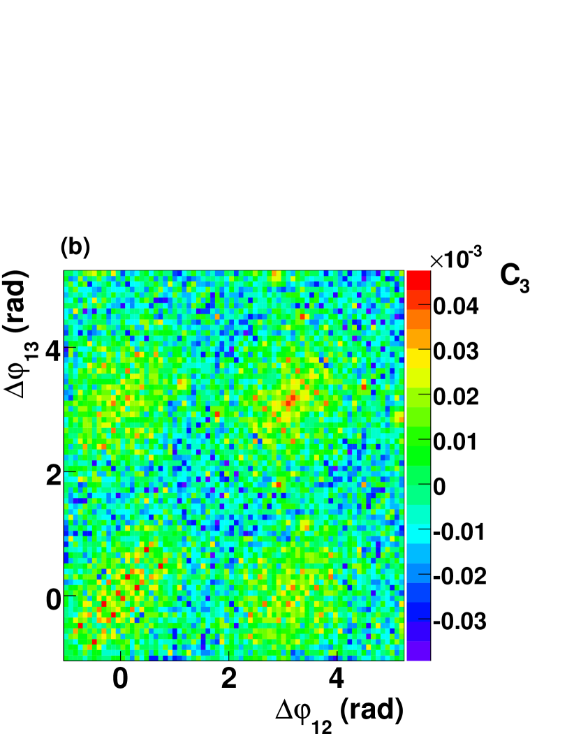
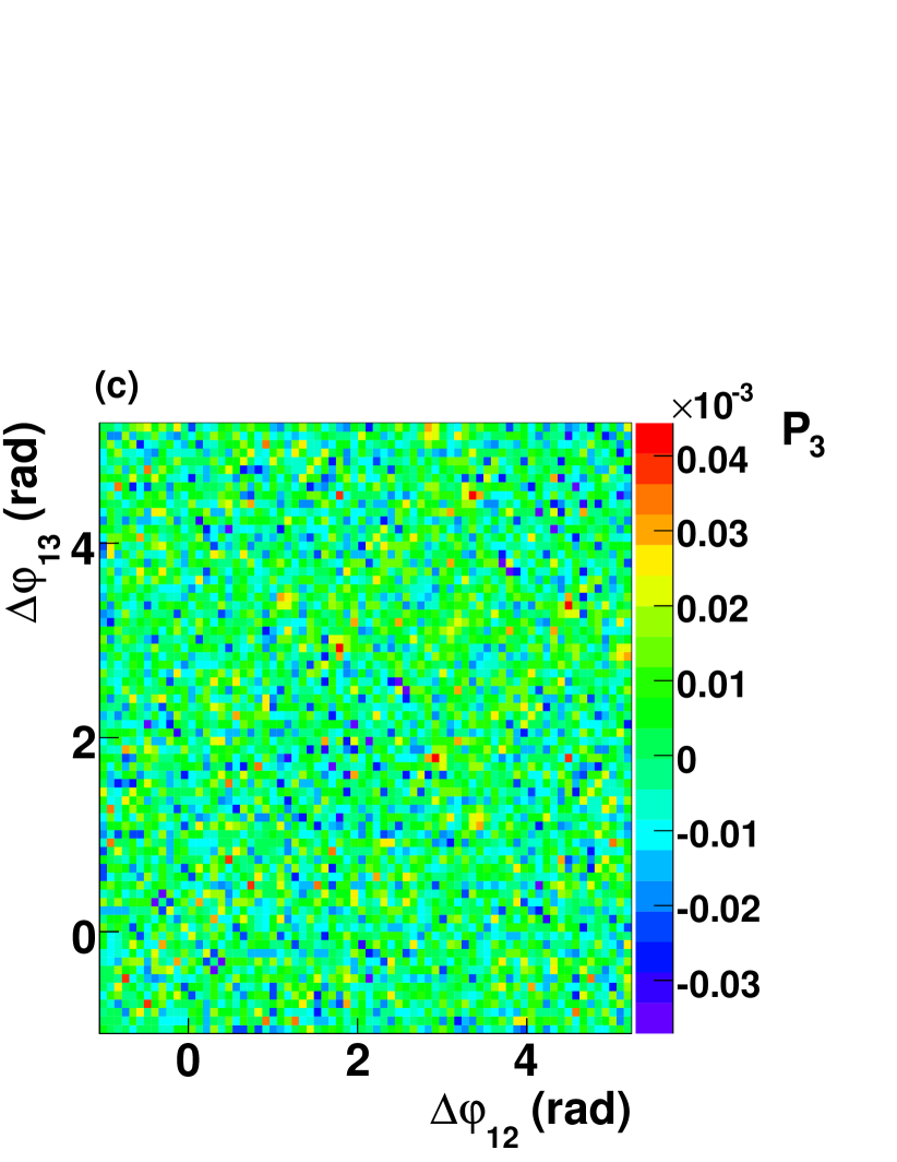
Figure 5: Simulations of (a) the three-particle density, (b) three-cumulant, and (c) the probability cumulant for particle emission with elliptic anisotropy $v_{2}$ = 0.10.

Figure 6 shows results of a simulation based on the same flow model as that used in Fig. 5, but with an added fourth harmonic component. Flow amplitudes are set to $v_{2}=0.1$ and $v_{4}=0.01$. While the 3-particle density (Fig 6 (a)) is completely dominated by the 2^nd harmonic, one finds the 3-cumulant suppresses this component significantly (Fig 6 (b)), and enables clear observation of the $v_{2}^{2}v_{4}$ non-diagonal terms expected from Eq. LABEL:probabilityCumulant. The $v_{2}^{2}$ component is further suppressed in the probability cumulant, shown in Fig 6 (c), where only the $v_{2}^{2}v_{4}$ component manifestly remains. As anticipated based on Eq. 39, the probability cumulant enables essentially full suppression of $v_{2}^{2}$ terms, and show irreducible flow components only.

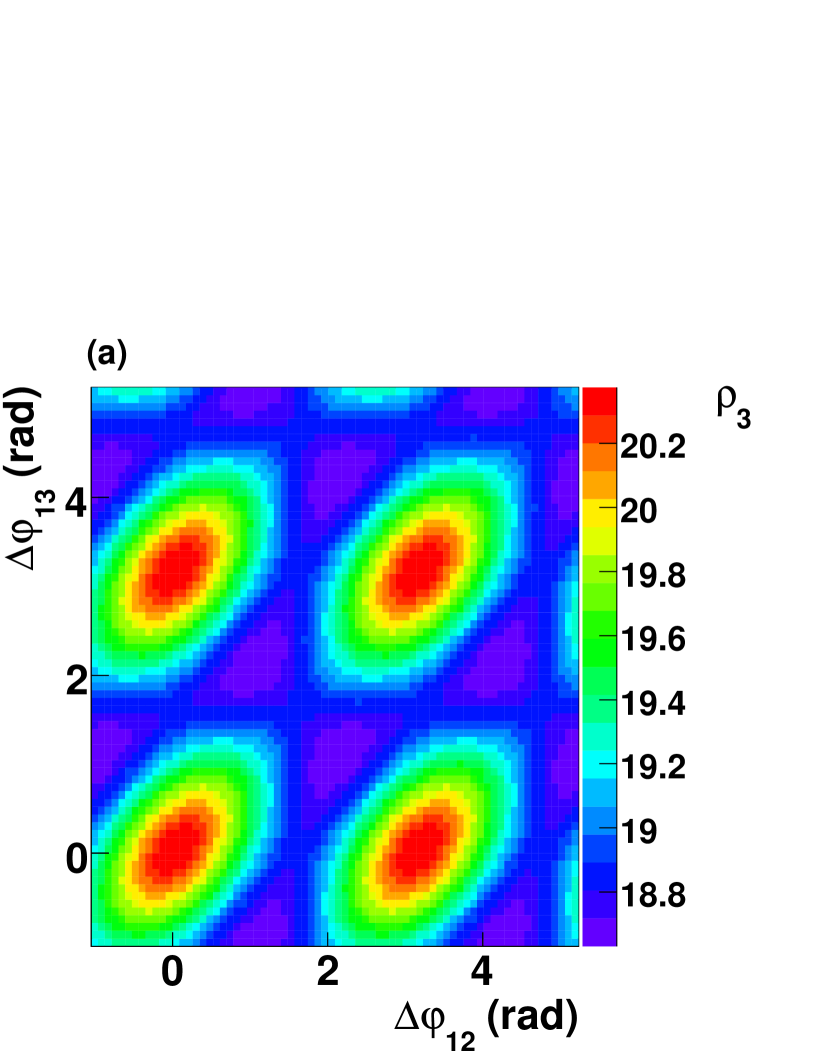
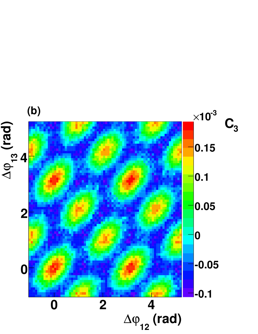
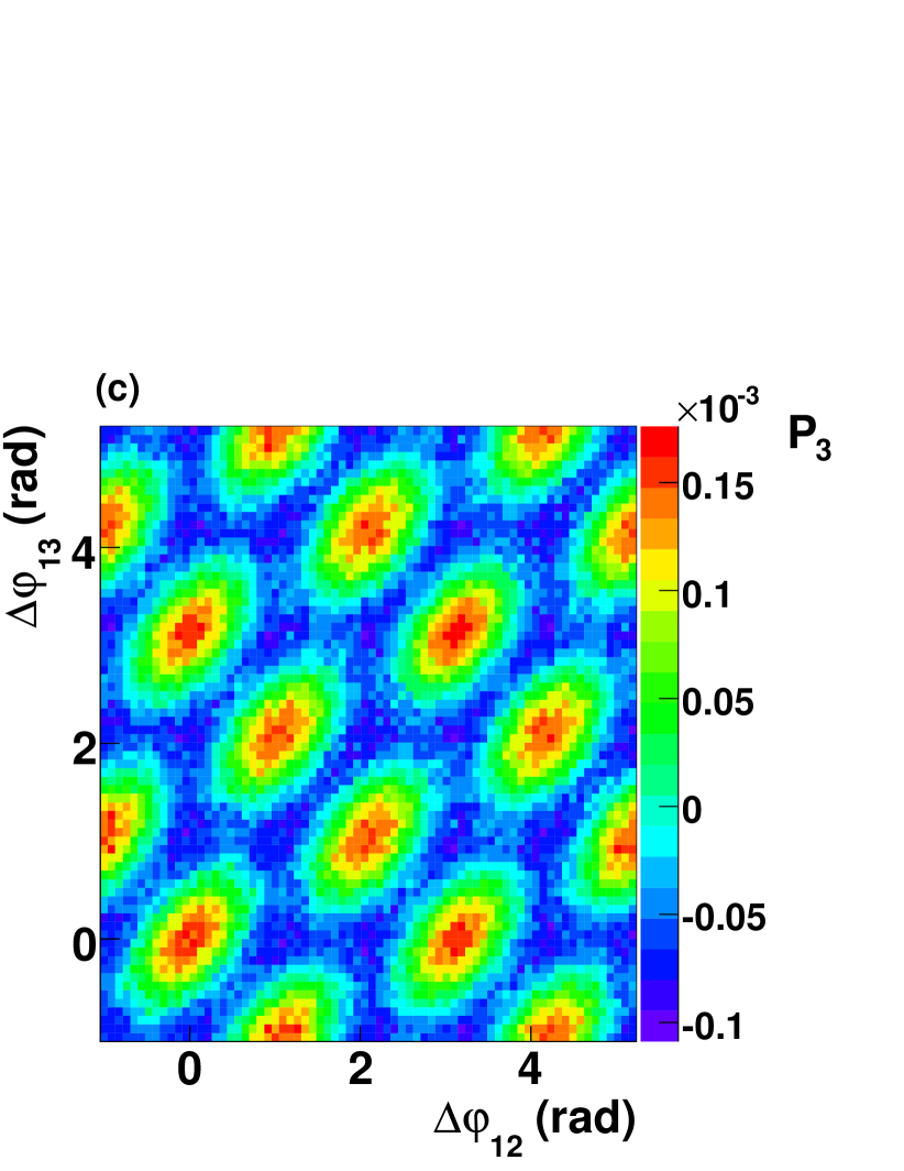
Figure 6: Simulations of (a) the three-particle density, (b) three-cumulant, and (c) the probability cumulant for particle emission with elliptic anisotropy $v_{2}=0.10$, and $v_{4}=0.01$.

Mono-jets and conical emission are next added to the simulated events. The jet axis (corresponding to the parton direction initiating the jet) is chosen randomly in the transverse plane. Particles are generated at random polar angles, relative to the jet direction using Gaussian PDFs. The width of the Gaussian is set to 0.15 radian for high $p_{t}$ particles, and 0.25 for low $p_{t}$ particles. Note that the conclusions of this study are essentially independent of the width of the jets. The associate multiplicity are generated jet-by-jet using Poisson PDFs. The near side jet associated particle multiplicity (i.e. number of associates per jet) are set to 1 and 2 for the high- and low-$p_{t}$ particles respectively. No away side jet is included. Instead, one introduces a conical emission as described in the following. Jet parameters are selected to correspond approximately to associate jet yields measured by the CDF collaboration for jets of 10 to 20 GeV CDF_JET , as well as jet associated yields reported by RHIC experiments Horner06 . The number of jets is generated event-by-event with a Poisson PDF of mean 0.01 jet per unit multiplicity: the average number of jets per event is thence of order 1-2. Such large values are used to ease our study. Smaller, perhaps more realistic jet-yield values result in a weaker signal. This limits the statistical significance of the measurement, but does not constitute an intrinsic limitation of the cumulant method.

In our simulations, the parton determining the direction of the jet is first generated, and is restricted for simplicity to the reaction transverse plane. The away-side parton is emitted in the transverse plane as well, at angle of $\pi$ radian relative to the jet parton. Conical emission is simulated by generating particles at a random polar angle relative to the away-side parton direction. The azimuthal direction of the particle, in the plane transverse to the parton direction, is randomly selected based on a uniform distribution. The polar angle is chosen to have a Gaussian distribution with an average value of one (1) radian. The number of high-$p_{t}$ particles produced in this cone is arbitrarily set to zero, while the number of low-$p_{t}$ cone particles in a given parton-parton collision is selected randomly with a Poisson distribution of mean equal two, unless specified otherwise in the following.

Because the cone particles are emitted at an arbitrary polar angle, but detected in the transverse plane as a function of relative azimuthal angles only, conical emission results in four Jacobian peaks, as seen in Fig. 7 (a). In order to characterize the shape and strength of these peaks, we use projections of the cumulants along the diagonals $\varphi_{12}+\varphi_{13}-2\pi$ and $\varphi_{12}-\varphi_{13}$. Projections, shown in Fig. 7 (b) are limited to include narrow angular ranges about the diagonals. Specifically, the range $|\varphi_{12}-\varphi_{13}|<10^{o}$ is integrated to obtain the projection along the plot main diagonal (displayed in red), whereas the condition $|(\varphi_{12}+\varphi_{13})-2\pi|<10^{o}$ is used for projections along $\varphi_{12}-\varphi_{13}$ (shown in blue).

At issue is whether or not one can extract a cone signal given the presence of background particles, and flow. We thus vary the strength of the jet signal to background ratio by changing the fractional jet and background yields. Figures 7 through 11 show cumulants and projections obtained with various model parameters. All plotted cumulants were obtained with simulations integrating two millions events.

Figures 7 (a-b) shows the cumulant and projections obtained for an average of 2.5 jets per event. The number of high and low $p_{t}$ particles associated with the jet, and cone are set respectively to 1 and 2. The uncorrelated background of high- and low-$p_{t}$ particle are set to 2.5 and 100 particles per event respectively. The cone signal obtained with such parameters is obviously strong and clearly observable. Figure 7 (c) displays the cumulant and projections with a high-$p_{t}$ background raised by a factor of 4 resuling in a signal to noise ratio of 25%. The observed cone strength remains unchanged, as expected given the background is uncorrelated. We also verified that an increase of the width of the gaussian PDF used for jet, and cone particle emission results in wider peak structures with reduced amplitude but no actual change in the integrated cone signal strenght. In this context, we conclude the observability of conical emission is only limited by the statistical accuracy of the measurement relative to the actual strength of the signal. For instantce, a reduction by a factor of five of the number of high-$p_{t}$ associated particles results in cone-signal five times small in amplitude, but the shape of the cumulant remains unchanged and the observability of the signal is thus only limited by the size of the event sample, and the number of particles associated with the trigger and cone.

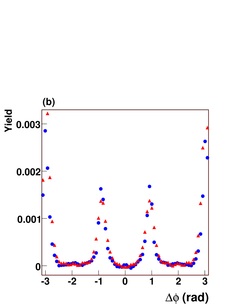
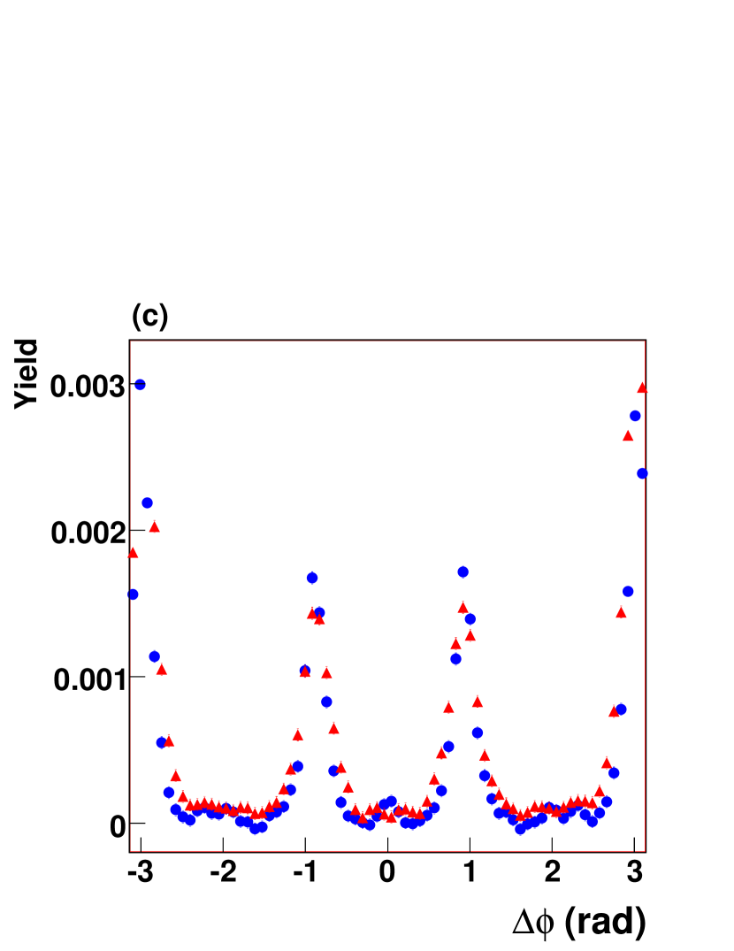
Figure 7: (a) Simulation of the 3-cumulant obtained with mono-jet, conical emission, and background particles (without flow). Average jet yield to high-$p_{t}$ particle background yield set to 1. (b) Projections of the cumulant along the main (red) and alternate (blue) diagonals for jet/cone parameters used in (a). Other particle generation parameters, and projections are discussed in the text. (c) Cumulant projections obtained for a high-$p_{t}$ background to jet-signal ratio of 4.

We next consider the observability of conical emission in the presence of anisotropic flow. Figure 8 shows the cumulant and projections in the presence of a flow background. The jet and conical signals are identical to those used in Fig. 7 (a-b). An average background of 100 low-$p_{t}$ particles is included with $v_{2}=0.1$, and $v_{4}=v_{2}^{2}$. No high-$p_{t}$ background is included. The cone signal shape and strength remains unaffected, although the projections exhibit a background structure somewhat more complex than that observed in Fig. 7. Fig. 8 (c) displays the projections obtained when the elliptic flow is raised to $v_{2}=0.2$. While the signal is clearly visible, one observes the emergences of cosine structures along the $\Delta\varphi_{23}$ projection. These stem from the non-Poisson nature of the background multiplicity fluctuations used in the simulations.

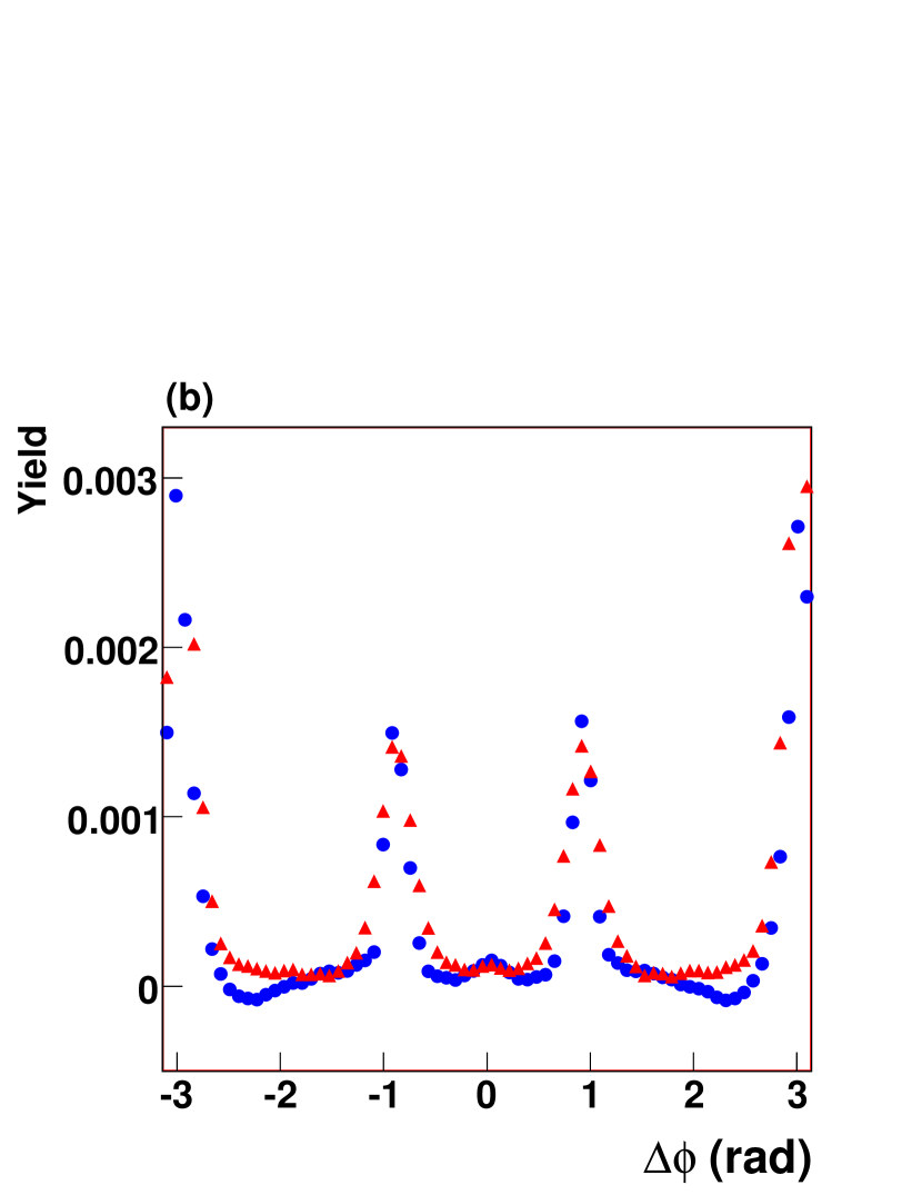
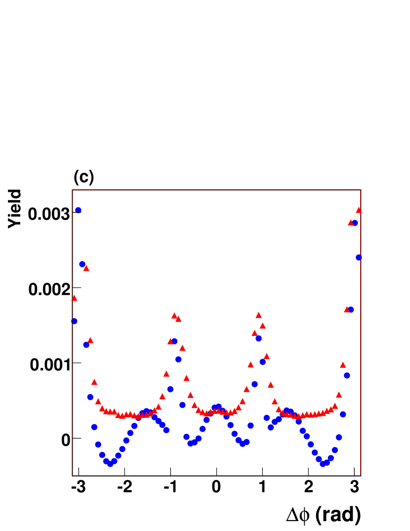
Figure 8: Idem Fig. 7 in the presence of background flow. (a-b) No background high-$p_{t}$ particle. Average of 100 low-$p_{t}$ background particle per event, with flow $v_{2}=0.1$, and $v_{4}=v_{2}^{2}$. (c) Average of 100 low-$p_{t}$ background particle per event, with flow $v_{2}=0.2$, and $v_{4}=v_{2}^{2}$.

Flow-like or cosine structures also appear when high-$p_{t}$ background particles are added as shown in Figure 9 where the average high-$p_{t}$ particle background is set to 2.5/event. The observability of the cone depends on its amplitude relative to that of the background, as well as on the magnitude of $v_{2}$ and $v_{4}$. We note that the signal remains visible in the $\Delta\varphi_{23}$ projection, with the jet and cone parameters used in Figure 7, even when the high-$p_{t}$ background is raised by a factor of eight as shown in Fig. 9. For substantially larger background, the signal however becomes more difficult to extract as illustrated in Figure 10 where a background to signal ratio of sixteen is used for high-$p_{t}$ particles. Clearly, the observability of a cone signal in the presence of flow depends on the strength of the signal relative to that of non-Poisson components and values of $v_{2}$.

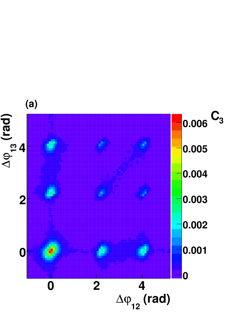
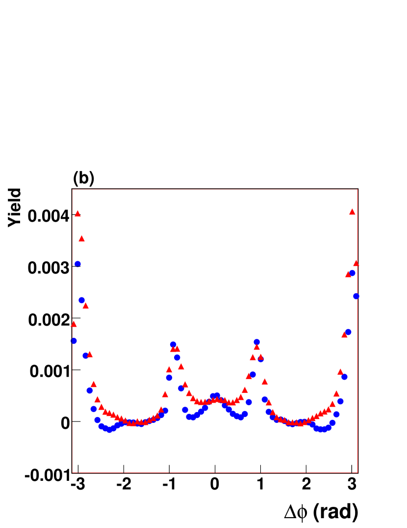
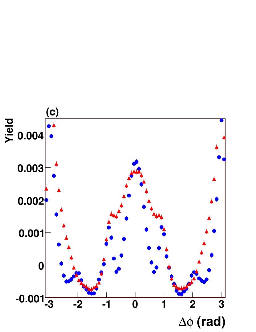
Figure 9: (a-b) Idem Fig. 7 for average jet yield to high-$p_{t}$ background equal one per event. Average of 100 low-$p_{t}$ background particle per event, with flow $v_{2}=0.1$, and $v_{4}=v_{2}^{2}$. (c) Projections obtained for average jet yield to high-$p_{t}$ background equal eight (8) per event.

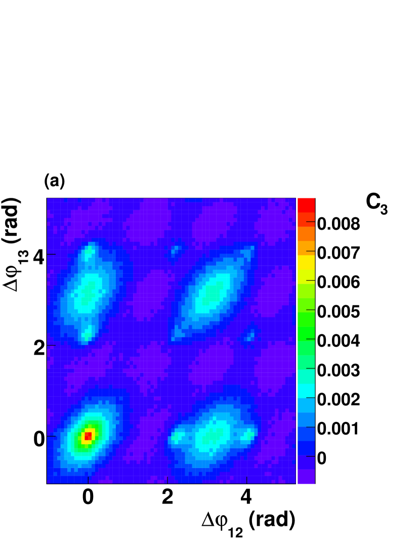
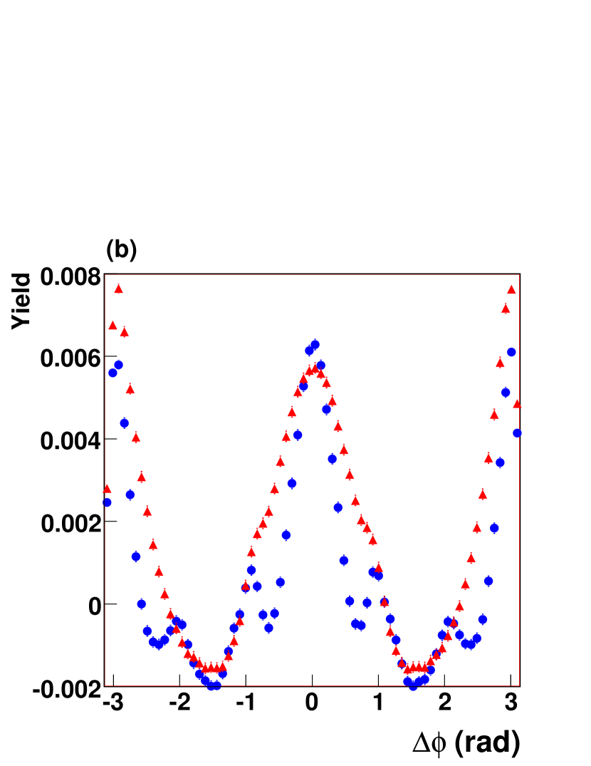
Figure 10: Idem Fig. 7 for average high-$p_{t}$ background to jet yield equal sixteen (16). Average of 100 low-$p_{t}$ background particle per event, with flow $v_{2}=0.1$, and $v_{4}=v_{2}^{2}$.

The model independent extraction of a conical signal becomes increasingly difficult as the signal strength is reduced and the elliptic flow magnitude increased. The measurement becomes particularly challenging when the jet amplitude is modulated by differential attenuation relative to the reaction plane, i.e. in the presence of jet-flow. Figures 11 (a) and (b) display projections along $\Delta\varphi_{1}2+\Delta\varphi_{1}3$ and $\Delta\varphi_{2}3$ obtained with jet $v_{2}=0.05$, (as defined in Sec. III.4). The blue squares and red circles show, respectively, the signals obtained with an average of two and one low-$p_{t}$ particles involved in conical emission. Simulations are carried out with an average number of 2.5 jets/cones per event. The average yield of high-$p_{t}$ low-$p_{t}$ background particle are set to 8 and 100 per event respectively. Background particles are produced with flow $v_{2}=0.1$, and $v_{4}=v_{2}^{2}$. In our simulation, the number of cone associated particles is determined event-by-event with a Poisson random number generator. The conical signal is detectable, in the context of this 3-cumulant analysis, only when two, or more, particles are generated per event. For an average cone yield of two associated particles, 60% of the cone events contain two or more cone particles. By contrast, only 26% of the events contain two cone particle when the average (cone) yield is one. The signal obtained in the former case is clearly visible, while if becomes weaker in the latter. The detectability of the signal thus greatly depends of the actual yield of conical emission. We note that two-particle correlation analyses report an away side yield of two particle per trigger after flow background subtraction based on a ZYAM hypothesis ZYAM . If this away side is due to conical emission, this implies the low-$p_{t}$ cone particle average multiplicity is large and should therefore be detectable in the context of a 3-cumulant analysis. We note however that the cumulant measurements reported by the STAR collaboration at recent conferences do not exhibit as strong $cos(2\Delta\varphi)$ components as those illustrated in the $\Delta\varphi_{1}+\Delta\varphi_{2}$ projections shown in Fig. 11 Pruneau06a . Note additionally that the cone signal remains visible in the $\Delta\varphi_{23}$ projection even for small signal to background ratios. It is however obvious that strong background flow and jet-flow may hinder the observation of conical emission. For instance, Figure 12 shows a comparison of the 3-cumulant projections obtained for conical emission in the presence of jet-flow cross terms with $v_{2}$ values of 0.05 (blue) and 0.1 (red) an associate cone yield of one. One finds the cone single is difficult to distinguish for $v_{2}=0.1$ but straightforward to observe for $v_{2}=0.05$.

In summary, e find in the context of our multicomponent model that the exact sensitivity of the measurement is a ”complicated” function of the flow and background parameters of the model, and cannot readily be expressed in analytical form or even as a table. We further note that the shape and strength of actual correlations is influenced by momentum, and quantum number conservation effects not explicitly addressed in this work.

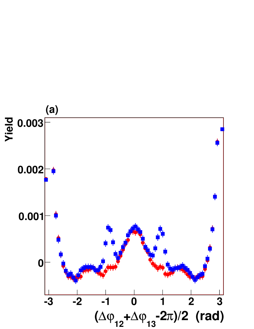
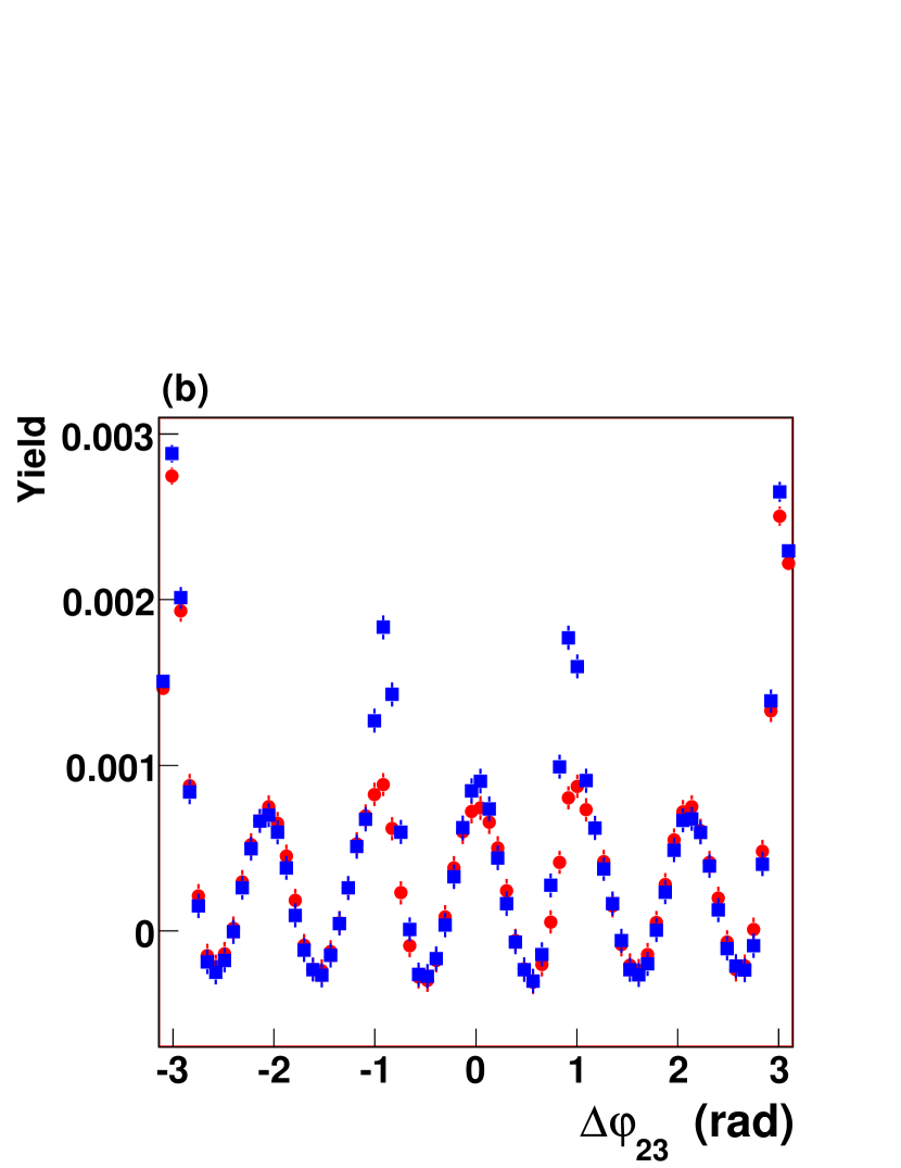
Figure 11: (Color online) Comparison of the cone signal obtained with an average of two (blue squares) and one (red circles) low-$p_{t}$ particles involved in conical emission. Panel (a) and (b) show the 3-cumulant projections along $(\Delta\varphi_{1}2+\Delta\varphi_{1}3)/2$ and $\Delta\varphi_{23}$ respectively. Simulations carried out with a jet-flow component, $v_{2}=0.05$, and an average number of 100 low-$p_{t}$ background particles per event, with flow $v_{2}=0.1$, and $v_{4}=v_{2}^{2}$. See text for details.

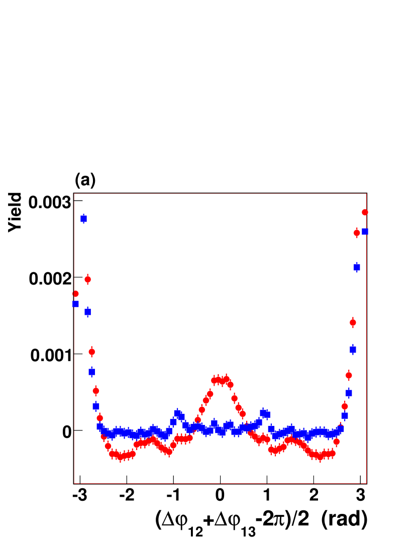
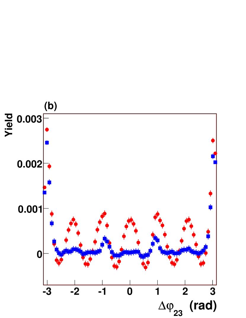
Figure 12: (Color online) Comparison of the cone signal obtained with an average of one low-$p_{t}$ particles involved in conical emission and an average of 100 low-$p_{t}$ background particles per event with $v_{2}=0.05$ (red circles) and $v_{2}=0.1$(blue squares). Panel (a) and (b) show the 3-cumulant projections along $(\Delta\varphi_{1}2+\Delta\varphi_{1}3)/2$ and $\Delta\varphi_{23}$ respectively. Simulations are carried out with a jet-flow component, $v_{2}=0.05$. The background has $v_{4}=v_{2}^{2}$.

VII Summary and Conclusions

Conical emission has been suggested in the recent literature to explain the away-side structures observed in two particle azimuthal correlations for $Au+Au$ collisions at $\sqrt{s_{NN}}=200$ GeV. If realized, conical emission should also lead to three particle correlations. We introduced in Ref. Pruneau06 a method based on cumulants to carry a search for such a signal. In this work, we presented a discussion of the properties of the three particle cumulant (3-cumulant) calculated in terms of two relative azimuthal angles, as defined in Pruneau06 , for searches of conical emission in high-energy $A+A$ collisions. We showed that in the presence of azimuthal anisotry (flow), the 3- cumulant reduces to non-diagonal terms dominated by components of order $v_{2}v_{2}v_{4}$ for Poissonian particle production. Given particle production is in general non-Poissonian, one however expects the presence of second order terms, dominated by components in $v_{2}^{2}$ in the cumulant. The strength of those terms relative to the irreducible $v_{2}v_{2}v_{4}$ components depends on the magnitude of $v_{2}$ and the global strength of particle correlations, or departure from Poisson statistics. The strength of particle correlation is known to vary inversely with the collision multiplicity in $A+A$ collisions due to increasing two-particle correlation dilution with increasing number of collision participants. We thus expect the mix of $v_{2}v_{2}v_{4}$ and $v_{2}^{2}$ should be a function of collision centrality.

We introduced a three-particle probability cumulant, and showed it is devoid of $v_{2}^{2}$ non-Poissonian components in the presence of flow only thereby enabling, in principle, the determination of $v_{2}v_{2}v_{4}$ amplitudes. We discussed the shape and strength of the 3-cumulant based on simple particle production models including di-jets, mono-jet plus conical emission, and jet$\times$flow correlations. We showed that jet$\times$flow cross-terms should be more complex than those assumed by some ongoing analyses, and cannot, in particular, be derived from a product of two-particle flow and jet-like terms. We used the models to discuss the sensitivity of the 3-cumulant for searches of conical emission in $A+A$ collisions. We showed that the cumulant enables excellent sensitivity to conical emission for modest values of flow $v_{2}$, but becomes increasingly challenging for larger values of $v_{2}$. We further showed that conical emission can be detected even in the presence of jet$\times$flow correlations for small values of $v_{2}$ jet flow. It is however obvious the signal may be masked by large values of jet and background $v_{2}$ and large non-Poissonian particle production. Precise values of sensitivity, in terms of signal strength to background ratios, cannot be expressed in a model independent way, and are found to depend on the relative amplitude of background $v_{2}$ and $v_{4}$ jet-flow correlations, as well as the global strength of particle correlations, i.e. departure from Poisson statistics.

This work neglects effects associated with momentum conservation, quantum number conservation, and particle correlations present in $p+p$ collisions. Momentum conservation implies in particular that a multicomponent description of particle production is not strictly valid, and while it is useful to estimate the effects of various particle production mechanisms, its use to search for conical emission signals is model dependent and therefore unreliable.

Acknowledgements

The author thanks S. Voloshin, M. Sharma, and A. Poskanzer for their critical reading of the manuscript, valuable comments and discussions. This work was supported in part by DOE Grant No. DE-FG02-92ER40713.

References

References

- (1) J. Hoffmann, H. Stoecker, U. Heinz, W. Scheid, and W. Greiner, Phys. Rev. Lett. 36, 88 (1976).
- (2) H. Stoecker, Nucl. Phys. A750, 121 (2005).
- (3) J. Ruppert, J. Phys. Conf. Ser. 27, 217 (2005).
- (4) J. Casalderrey-Solana, E. V. Shuryak, and D. Teany, J. Phys. Conf. Ser. 27, 22 (2005).
- (5) J. Ruppert, B. M ller, Physics Letters B618, 123 (2005).
- (6) T. Renk and J. Ruppert, Phys. Rev. C 73, 011901 (2006).
- (7) A. K. Chaudhuri, U. W. Heinz, Phys. Rev. Lett. 97, 062301 (2006).
- (8) H. Stocker, et al. nucl-th/0703054, 2007.
- (9) T. Renk, J. Ruppert, hep-ph/0702102.
- (10) B. Muller, J. of Physics G: Nucl. Part. Phys. (QM 08 Proceedings) in press.
- (11) B. Betz, J. of Physics G: Nucl. Part. Phys. (QM 08 Proceedings) in press.
- (12) S. Mukherjee, M. Mustafa, and F. Ray, Phys. Rev. D 75, 094015 (2007).
- (13) S. Gubser, S. Pufu, and A. Yarom, Phys. Rev. Lett. 100 012301. (2008).
- (14) I.M. Dremin, JETP Lett. 30 140 (1979).
- (15) I.M. Dremin, Sov. J. Nucl. Phys.33 726 (1981).
- (16) I.M. Dremin, Nucl. Phys. A 767, 233 (2006).
- (17) V. Koch, A. Majumber, X.-N. Wang, Phys. Rev. Lett. 96, 172302 (2005).
- (18) A. Majumder, B. Muller, S. A. Bass (2006), hep-ph/0611135.
- (19) I. Vitev, Phys. Lett. B 630, 78 (2005).
- (20) A.D. Polosa and C.A. Salgado, hep-ph/0607295.
- (21) C. B. Chiu, R. C. Hwa, Phys. Rev. C74, 064909 (2006).
- (22) N. Armesto, et al., Phys. Rev. Lett. 93, 242301 (2004), hep-ph/0405301.
- (23) N. Armesto, C.A. Salgado, U. A. Wiedemann, Phys. Rev. C 72, 064910 (2005).
- (24) T. Renk and J. Ruppert, Phys. Lett. B646, 19 (2007).
- (25) T. Renk and J. Ruppert, Phys. Rev. C76, 014908 (2007).
- (26) S.A. Voloshin, Phys. Lett. B 632, 490 (2006) arXiv:nucl-th/0312065.
- (27) C. B. Chiu, R. C. Hwa, Phys. Rev. C72, 034903 (2005), nucl-th/0505014.
- (28) W. G. Holzmann, N. N. Ajitanand, J. M. Alexander, P. Chung, M. Issah, R. A. Lacey, A. Taranenko and A. Shevel, J. Phys. Conf. Ser. 27, 80 (2005).
- (29) Chun Zhang et al. (PHENIX Collaboration), J. of Physics G: Nucl. Part. Phys. 34, S671 (2007).
- (30) J. Ulery, et al. (STAR Collaboration), Nucl. Phys. A 774, 581 (2006).
- (31) J. Ulery and F. Wang, nucl-ex/0609016.
- (32) J. Ulery, et al. (STAR Collaboration), nucl-ex/07040224.
- (33) J. Ulery, Ph.D. Thesis, Purdue University, (2007).
- (34) N.N. Ajitanand (PHENIX Collaboration), Nucl. Phys. A774 585 (2006).
- (35) J. Ulery, et al. (STAR Collaboration), Nucl. Phys. A 783, 511 (2007).
- (36) Stefan Kniege and Mateusz Ploskon, et al. (CERES Collaboration), J. of Physics G: Nucl. Part. Phys. 34, S697 (2007).
- (37) S. Kniege, M. Ploskon (CERES Collaboration), nucl-ex/0703008.
- (38) N. N. Ajitanand, Nucl. Phys. A783 519 (2007).
- (39) N. Borghini, Phys.Rev. C75 (2007) 021904.
- (40) Zbigniew Chajecki, and Mike Lisa, arXiv:0807.3569.
- (41) C. A. Pruneau, Phys. Rev. C74 064910 (2006).
- (42) C. Pruneau, et al. (STAR Collaboration), J. of Physics G: Nucl. Part. Phys. 34, S667 (2007).
- (43) E. L. Berger, Nucl. Phys. B85, 61 (1975)..
- (44) P. Carruthers and I. Sarcevic, Phys. Rev. Lett. 63, 1561 (1989).
- (45) M. Anderson et al. (STAR Collaboration), Nucl. Instrum. Meth. A 499 659 (2003).
- (46) STAR Collaboration, private communication.
- (47) T. Affolder, et al. STAR Collaboration, Phys. Rev. D 65, 092002 (2002).
- (48) I. Arsene et al. BRAHMS Collaboration, Nucl. Phys. A 757, 1 (2005); K. Adcox et al. PHENIX Collaboration, ibid . 184; B. B. Back et al. PHOBOS Collaboration, ibid . 28; J. Adams et al. STAR Collaboration, ibid . 102.
- (49) J. Adams et al. STAR Collaboration, Phys. Rev. C 72, 014904 (2005).
- (50) S. A. Voloshin, A. M. Poskanzer, and R. Snelling, nucl-ex/0809.2949.
- (51) N. N. Ajitanand, et al. Phys.Rev. C 72, 011902(2005).
- (52) M. Horner, et al. (STAR Collaboration), J. of Physics G: Nucl. Part. Phys. 34, S995 (2007).