Hilbert Space Average Method and adiabatic quantum search

Abstract

We discuss some aspects related to the so-called Hilbert space Average Method, as an alternative to describe the dynamics of open quantum systems. First we present a derivation of the method which does not make use of the algebra satisfied by the operators involved in the dynamics, and extend the method to systems subject to a Hamiltonian that changes with time. Next we examine the performance of the adiabatic quantum search algorithm with a particular model for the environment. We relate our results to the criteria discussed in the literature for the validity of the above-mentioned method for similar environments.

I Introduction

The study of open quantum systems has attracted renewed attention during the last years. One important reason for this is the expected advent of future quantum computers Chuang . The interaction of the quantum computer with its surroundings can introduce some degree of decoherence which can, eventually, ruin the performance of the quantum algorithm. Although this phenomenon can be mitigated with the help of error-correction methods, a deeper understanding of how the ambiance operates on the smaller system can also be used to improve the working conditions. In fact, recent papers have shown that, for some models of system-ambiance interaction, the loss of coherence can be smaller if the ambiance temperature is increased Amin ; Montina . Similarly, designing some engineered reservoirs with controlled coupling and state of the environment can reduce the decoherence rate Cui ; Gordon . One can even consider purely dissipative processes, which turn out to be equivalent to a quantum circuit model for quantum computation Verstraete . On the other hand, systems subject to decoherence will experience a transition from a quantum to a classical state. The study of this transition will give more insight about the nature of Quantum Mechanics and its differences with a classical perception Ollivier .

There are different approaches which have been developed in the literature in order to describe the evolution of open systems, based on different techniques such as master equations or superoperators Breuer . As an alternative to these methods, we will study the behavior of the open system using the so-called Hilbert space Average Method (HAM, in what follows) Michel ; Gemmer . This method has been proved to give, in some situations, better results than conventional Time Convolutionless (TCL) approximations, and comparable to correlated projection superoperator techniques Breuer06 . We will extend this approach to the case of a time-varying Hamiltonian acting on the open system, and will show that, under a suitable choice of the operators defining the HAM scheme, the resulting equations will adopt the form of traditional master equations, at least up to second order in the system-environment coupling.

As an application, we will consider the case of a quantum system which is designed to perform a Grover search Grover ; Boyer ; Grover2 via adiabatic quantum computation Farhi2 ; Farhi3 ; Roland ; Das . Our purpose is to analyze the response of the quantum computer when coupled to the external influence of an environment, introduced with the help of some specific model. This problem has been considered by several authors Amin ; Childs ; Sarandy ; Ashhab ; Amin08 ; Tiersch ; Perez07 ; Aabergrc ; Aaberg ; Johansson , but here we relate it to similar models for the bath which have discussed within the HAM formalism. We compare our results with a numerical simulation of the Schrödinger equation obeyed by the full system.

In Section II we introduce some basic notations. In Sect. III we briefly revisit the HAM method, using an approach that makes not use of the algebra of the involved operators. An approximated evolution equation, extended to the case of a time-changing Hamiltonian acting on the system, is obtained in Sect. IV, and we also make a connection with familiar master equations. Sect. V is devoted to the analysis of adiabatic search when the quantum computer interacts with a particular environment. The evolution of the system is followed both by the exact Schrödinger equation and by solving the obtained approximated equations. The comparison of both calculations is discussed within the framework of known criteria for similar models, which have derived within the HAM formalism. Our results are summarized on Sect. VI.

We work in units such that $\hbar=1$.

II basic notations

We wish to study the evolution of an open system (S) in contact with an environment (E). First we introduce the basic quantities in the Schrödinger picture, and then we will define a convenient interaction picture for this problem. System S is subject to a time-dependent Hamiltonian $H_{S}(t)$ . Let us denote by $H_{E}$ the Hamiltonian describing the free evolution of the environment, and by $V$ the interaction between both systems. Both $H_{E}$ and $V$ are assumed to be time-independent. Moreover, we make the hypothesis that $[H_{S}(t),H_{E}]=0$ . The evolution of the density matrix $\rho(t)$ of the complete (S+E) system is therefore given by

$$\frac{d}{dt}\rho(t)=-i[H(t),\rho(t)]$$ (1)

with $H(t)=H_{S}(t)+H_{E}+V$ the total Hamiltonian. We can define an interaction picture density matrix $\rho_{I}(t)$ as follows:

$$\rho_{I}(t)\equiv\exp(iH_{E}t)\rho(t)\exp(-iH_{E}t).$$ (2)

The equation for $\rho_{I}(t)$ is easily obtained:

$$\frac{d}{dt}\rho_{I}(t)=-i[H_{S}(t),\rho_{I}(t)]-i[V_{I}(t),\rho_{I}(t)],$$ (3)

where

$$V_{I}(t)\equiv\exp(iH_{E}t)V\exp(-iH_{E}t)$$ (4)

is the interaction operator in the interaction picture. In what follows we will assume, unless otherwise specified, that we are working in the above-defined picture, and will therefore omit the subscript ’I’.

III Hilbert Space Average method

In this section we briefly review the Hilbert space Average Method (HAM), as an alternative to describe the dynamics of an open quantum system. A more detailed description of the method can be found in Michel ; Breuer06 ; Gemmer .

The idea is to replace the dynamics of the density matrix $\rho(t)$ describing the full system (i.e. open system plus reservoir) by an effective density matrix $\alpha(t)$ which is simpler to describe, with the condition that the expected values of a given set of operators is reproduced. Let us assume that we are interested on a set of operators $\{\hat{P}_{n}\}$ and we want to define a density matrix satisfying the boundary conditions

$$Tr[\alpha(t)\hat{P}_{n}]\equiv p_{n}(t),$$ (5)

where the functions $p_{n}(t)$ are assumed to be known (actually, they will be determined by the dynamics), and $Tr$ stands for the trace over the whole Hilbert space. We would like to determine $\alpha(t)$ respecting the above conditions, but otherwise unknown. To this end we establish the following procedure. We maximize the entropy, in order to account for our ignorance about the effective density matrix, but add constraints corresponding to Eqs. (5) under the form of Lagrange multipliers. For our purpose, it is simpler to consider the linear entropy $S[\rho]=1-Tr[\rho^{2}]$. In this way, we find the extrema of the functional

$$I[\alpha]\equiv S[\alpha]-\sum_{n}a_{n}Tr[\alpha\hat{P}_{n}]$$ (6)

with $\{a_{n}\}$ the above defined Lagrange multipliers. Following this procedure, one arrives to the expression

$$\alpha(t)=\sum_{n}b_{n}(t)\hat{P}_{n},$$ (7)

with $b_{n}=-a_{n}/2$ , and we have made explicit the time dependence of $\alpha(t)$ . The new functions $b_{n}(t)$ are determined by Eqs (5). Of course, one also has to make sure that the condition $Tr[\alpha(t)]=1$ is satisfied.

In Michel ; Breuer06 ; Gemmer , the authors introduce the HAM method as an average over all possible states in the Hilbert space that accounts for conditions Eqs. (5) (here is where the name HAM comes from), and introduce the set of operators $\{\hat{P}_{n}\}$ as obeying a closed algebra. In contrast, our derivation of Eq. (7), although perhaps less intuitive, makes no use of the algebra of the operators $\{\hat{P}_{n}\}$ .

IV Approximated evolution equation

The exact dynamics of $\alpha(t)$ will be given by solving an equation like Eq. (3) in the interaction picture. This equation does not admit a simple, closed form, solution. In this section we will investigate some approximation that is easier to solve, and will allow us to make a connection with standard master equations. We first introduce the evolution operator $U(t+\tau,t)$ from instant $t$ to $t+\tau$. We then have

$$\alpha(t+\tau)=U(t+\tau,t)\alpha(t)U^{\dagger}(t+\tau,t).$$ (8)

In order to separate the evolution due to $H_{s}(t)$ from that due to $V(t)$ we consider a sufficiently small $\tau$ and approximate $U(t+\tau,t)$ by a second-order Suzuki decomposition Suzuki

$$U(t+\tau,t)\simeq\exp(-i\frac{\tau}{2}H_{S}(t))D_{V}(t+\tau,t)\exp(-i\frac{\tau}{2}H_{S}(t)),$$ (9)

where $D_{V}(t+\tau,t)$ is the evolution operator describing the time evolution due to $V(t)$ alone (i.e., neglecting $H_{S}(t)$ in the Hamiltonian), and verifies the equation

$$i\frac{d}{dt}D_{V}(t,t_{0})=V(t)D_{V}(t,t_{0})$$ (10)

Inserting Eq. (9) into (8) and expanding the exponentials in powers of $\tau$ gives

$$\alpha(t+\tau)=\alpha(t)+\Delta\alpha(t+\tau,t)+i\tau[\alpha(t),H_{S}(t)]+\mathcal{O}(\tau^{2}),$$ (11)

with the definition

$$\Delta\alpha(t+\tau,t)\equiv D_{V}(t+\tau,t)\alpha(t)D_{V}^{\dagger}(t+\tau,t)-\alpha(t).$$ (12)

We now would like to make an approximate treatment of the quantity $\Delta\alpha(t+\tau,t)$ defined in the latter equation. To this purpose, we use the solution of Eq. (10) up to second order in the potential

$$D_{V}(t+\tau,t)\simeq I-i\int_{t}^{t+\tau}dsV(s)-\int_{t}^{t+\tau}ds\int_{t}^{s}ds^{\prime}V(s)V(s^{\prime}).$$ (13)

Within this approximation, Eq. (12) reads

$$\Delta\alpha(t+\tau,t) = -i\int_{t}^{t+\tau}ds[V(s),\mbox{}\alpha(t)]$$ (14)

$$-\int_{t}^{t+\tau}ds\int_{t}^{s}ds^{\prime}[V(s),[V(s^{\prime}),\alpha(t)]]\,.$$

Starting from this approximation, one can derive the corresponding equations for the functions $\{p_{n}(t)\}$ , following the procedure described in Michel . To this end, one needs to specify the operators $\{\hat{P}_{n}\}$ and the algebra verified by them.

We can also establish a connection with familiar master equations, which is done in a trivial way within the above formalism. We simply assume that the effective density matrix $\alpha(t)$ can be factorized as

$$\alpha(t)=\rho_{S}(t)\otimes\rho_{E}$$ (15)

where $\rho_{E}$ is a density matrix that approximates the state of the bath, and $\rho_{S}(t)$ is the density matrix for the system S, related to $\alpha(t)$ via

$$\rho_{S}(t)=Tr_{E}[\alpha(t)],$$ (16)

and $Tr_{E}$ indicates the partial trace over the environment E.

Let us introduce an orthonormal basis $\{|i>\}$ in the Hilbert space corresponding to system S, and write Eq. (15) in the following way:

$$\alpha(t)\equiv\sum_{i,j}P_{ji}(t)|i><j|\otimes\rho_{E}$$ (17)

By comparing with Eq. (7) we identify the operators $\hat{P}_{n}$ associated with the ansatz (15)

$$\hat{P}_{n}=|i><j|\otimes\rho_{E}$$ (18)

where $n$ indicates a given pair $i,j$. One also easily obtains from Eq. (5) that

$$p_{n}(t)=P_{ij}(t)Tr[\rho_{E}^{2}].$$ (19)

Notice that the functions $P_{ij}(t)$ are related to the matrix elements $\rho_{Si,j}(t)$ in the basis $\{|i>\}$ via $P_{ij}(t)=\rho_{Sji}(t)$ .

In order to obtain a more detailed expression for the quantity $\Delta\alpha(t+\tau,t)$ one needs to specify the interaction $V$ . Let us assume that this operator is defined, in the Schrödinger picture, by

$$V=\sum_{i}A_{i}\otimes C_{i}$$ (20)

with the Hermitian operators $A_{i}$ ($C_{i}$) acting on the system S (E). Of course, one can consider a more general situation where these operators are not Hermitian, and simply add the Hermitian conjugate to $V$ . However, a simplified version like Eq. (20) will be sufficient to our purposes. In the interaction picture, the above formula becomes

$$V_{I}(t)=\sum_{i}A_{i}\otimes C_{i}(t)$$ (21)

with $C_{i}(t)\equiv\exp(iH_{E}t)C_{i}\exp(-iH_{E}t)$ . Hereafter, we omit the subindex ’I’, as anticipated in Sect. II, and assume that we are working in the interaction picture.

In what follows, we are interested in the difference

$$\Delta\rho_{S}(t+\tau,t)\equiv\rho_{S}(t+\tau)-\rho_{S}(t)=Tr_{E}[\Delta\alpha(t+\tau,t)].$$ (22)

We will obtain an approximation to this quantity by using Eqs. (14) and (21). The rest of this section is a standard manipulation which is common to the derivation of master equations. Our purpose is only to show that the program we started in Sect. III does indeed lead to such kind of equations. The interested reader is addressed to the existing bibliography (see, e.g. Breuer ). The final expression reads

$$\frac{d}{dt}\rho_{S}(t) = -i[H_{S}(t),\rho_{S}(t)]$$ (23)

$$+ \frac{1}{2}\sum_{l,k}\Gamma_{lk}(t)\{A_{k}\rho_{S}(t)A_{l}-A_{l}A_{k}\rho_{S}(t)\}+\mathrm{h.c.}$$

where the Hermitian conjugate refers only to the summation. In obtaining Eq. (23) we have taken the limit $\tau\rightarrow 0$ , and we have defined

$$\Gamma_{lk}(t)=\lim_{\tau\rightarrow 0}\frac{2}{\tau}\int_{t}^{t+\tau}ds\int_{t}^{s}ds^{\prime}G_{lk}(s,s^{\prime}),$$ (24)

with

$$G_{lk}(s,s^{\prime})\equiv Tr_{E}\{C_{l}(s)C_{k}(s^{\prime})\rho_{E}\}$$ (25)

the bath correlation functions. We also have made the usual hypothesis Breuer that

$$Tr_{E}\{C_{l}(s)\rho_{E}\}=0.$$ (26)

Eq. (23) takes then the familiar form of a master equation, which becomes of the Lindblad type in the case that the coefficients $\Gamma_{lk}(t)$ are independent of time.

V Model for adiabatic search and interaction with the environment.

We now analyze a particular and interesting example, which can be cast either under the form of HAM or master equations, according to the discussion of the previous section. We study the performance of an open quantum system (the quantum computer) consisting on $n$ qubits, while it does an adiabatic search for a marked state $|m>$ out of $N=2^{n}$ possible configurations, subject to the interaction with an environment. This problem has been addressed by several authors Amin ; Childs ; Sarandy ; Ashhab ; Amin08 ; Tiersch ; Perez07 ; Aabergrc ; Aaberg ; Johansson . Here, we relate the problem to similar bath models which have derived within the HAM formalism.

The Hamiltonian $H_{S}(t)$ implements the adiabatic quantum search, and will be written as

$$H_{S}(t)=f(t)(I-|\Psi_{0}><\Psi_{0}|)+g(t)(I-|m><m|)$$ (27)

where $|\Psi_{0}>$ corresponds to the initial state of the system, which we take as the equally-weighted superposition $|\Psi_{0}>=\frac{1}{\sqrt{N}}\sum_{i=1}^{N}|i>$ and $I$ is the identity operator. The functions $f(t)$ and $g(t)$ will vary slowly during the running time $t_{G}$, and satisfy $f(0)=1$, $g(0)=0$ , $f(t_{G})=0$, $g(t_{G})=1$. There are many possible choices of these functions, depending on the trade-off between time and energy cost one pursues Roland ; Das ; Perez07 . Here we choose these functions as obtained form imposing a local adiabatic condition Roland , with $f(t)=1-s(t)$ , $g(t)=s(t)$ . In the large $N$ limit

$$s(t)=\frac{1}{2}+\frac{1}{2\sqrt{N}}\tan(\frac{2\epsilon t}{\sqrt{N}}-\arctan\sqrt{N}),$$ (28)

where $\epsilon$ is a small number that controls the probability of success for the algorithm, which will run during a time $t_{G}=\pi\sqrt{N}/2\epsilon$.

The adiabatic quantum search evolution can be effectively reduced to a two-level system, in the space spanned by the orthogonal vectors $\{|m>,|p>\}$ , with $|p>=\frac{1}{\sqrt{N-1}}\sum_{i\neq m}|i>$. The minimum energy gap in the Hamiltonian (27) appears for eigenstates which are linear combinations of $\{|m>,|p>\}$ . It occurs when $s(t)\simeq 1/2$ and takes the value $1/\sqrt{N}$. The rest of eigenvectors are degenerate, with eigenvalue $f+g=1$, and are well separated from the previous two, specially around the avoided crossing point $s\simeq 1/2$. It is reasonable to assume that one can restrict the system evolution to this effective two-level space. Arguments to favour this assumption are shown in Amin08 .

We now introduce a model to describe the interaction with the environment. We will make an explicit comparison with a numerical simulation of the Schrödinger equation. To this end, we make use of a simple model consisting on a band of $N_{1}$ equally spaced levels. As we show, this model can describe relaxation to equilibrium and decoherence effects in a natural way, and may be regarded as a simplified version of the two-band model described in Breuer06 . The Hamiltonian describing the environment is given by

$$H_{E} = \sum_{n=1}^{N_{1}}\frac{\delta\varepsilon}{N_{1}}n|n\rangle\langle n|$$ (29)

and the interaction between both systems by

$$V=\sum_{i=1}^{n}\sigma_{+}^{i}B_{i}+{\mbox{h.c.}},$$ (30)

with

$$B_{i}=\lambda_{i}\sum_{n_{2}>n_{1}}c_{i}(n_{1},n_{2})|n_{1}\rangle\langle n_{2}|.$$ (31)

The indices $n,n_{1}$ and $n_{2}$ label the levels of the energy band, and $\sigma_{+}^{i}$ are Pauli matrices acting on qubit $i$ . The global strength of the interaction with each one of the qubits is given by $\lambda_{i}$. The coupling constants $c_{i}(n_{1},n_{2})$ are independent Gaussian random variables. In order to make the model simpler, we will choose the same couplings for all qubits, which amounts to the replacement $\sum_{i=1}^{n}\lambda_{i}c_{i}(n_{1},n_{2})\rightarrow n\lambda c(n_{1},n_{2})$ in Eq. (30). The averages (denoted by $<>$) over the random constants $c(n_{1},n_{2})$ satisfy:

$$\langle c(n_{1},n_{2})\rangle = 0,$$ (32)

$$\langle c(n_{1},n_{2})c(n^{\prime}_{1},n^{\prime}_{2})\rangle = 0,$$ (33)

$$\langle c(n_{1},n_{2})c^{*}(n^{\prime}_{1},n^{\prime}_{2})\rangle = \delta_{n_{1},n^{\prime}_{1}}\delta_{n_{2},n^{\prime}_{2}}.$$ (34)

We will assume that an average over the possible realizations of these coefficients is made when evaluating Eq. (25).

Up to now, our model describes the coupling of the $n$ qubits of the quantum computer to the environment. According to the above discussion, we will make the assumption that only the subspace spanned by the states $\{|m>,|p>\}$ is relevant for the dynamics. Accordingly, we need to compute the matrix elements of Eq. (30) in this basis. A straightforward calculation gives, in the limit of large $N=2^{n}$:

$$V=\sigma_{z}C,$$ (35)

where $\sigma_{z}$ acts on the system subspace, and

$$C=-\frac{1}{4}\sum_{i=1}^{n}(B_{i}+B_{i}^{\dagger})$$ (36)

acts on system E. In the interaction picture, the above operator becomes

$$C(t)=-\frac{n\lambda}{4}\sum_{n_{2}>n_{1}}c(n_{1},n_{2})e^{-it\omega(n_{1},n_{2})}|n_{1}\rangle\langle n_{2}|+h.c.,$$ (37)

with $\omega(n_{1},n_{2})=\frac{\delta\varepsilon}{N_{1}}(n_{2}-n_{1})$ .

The interaction Hamiltonian Eq. (35) is of the general form (20), with only one term appearing. Consequently, only one correlation function arises, which we represent by $G(s,s^{\prime})$ . Associated to this function, it exists one function $\Gamma(t)$ defined as in (24). One can also check that condition (26) is satisfied.

As for the state $\rho_{E}$ , we make the simplest choice, by taking $\rho_{E}=\frac{I_{E}}{N_{1}}$ , where $I_{E}$ is the identity operator in the environment space. This choice obviously satisfies $[H_{E},\rho_{E}]=0$ . As a consequence, the correlation function $G(s,s^{\prime})$ only depends on the difference $s-s^{\prime}$ , and the function $\Gamma(t)$ becomes independent of $t$ . A redefinition of the variables $s$ and $s^{\prime}$ gives

$$\Gamma=\lim_{\tau\rightarrow 0}\frac{2}{\tau}\int_{0}^{\tau}ds\int_{0}^{s}ds^{\prime}G(s^{\prime}).$$ (38)

The correlation function can be calculated straightforwardly in the present model. We will consider the limit $N_{1}\gg 1$ . In this limit, one obtains

$$G(s)=N_{1}(\frac{n\lambda}{2\delta\varepsilon s}\sin\frac{\delta\varepsilon s}{2})^{2}.$$ (39)

The evaluation of the limit in Eq. (38) deserves some discussion. As will be shown below, we will be interested in time intervals which are much larger than $1/\delta\varepsilon$ . For such long-time variations, we can still consider values of $\tau$ that are larger than $1/\delta\varepsilon$, i.e. we assume that $\tau\delta\varepsilon\gg 1$ (see Michel for an extensive discussion). Within this context, Eq. (38) finally gives

$$\Gamma=\frac{n^{2}\lambda^{2}\pi N_{1}}{8\delta\varepsilon}.$$ (40)

The master equation (23) can be finally written, for our model, as

$$\frac{d}{dt}\rho_{S}(t)=-i[H_{S}(t),\rho_{S}(t)]+\Gamma(\sigma_{z}\rho_{S}(t)\sigma_{z}-\rho_{S}(t)).$$ (41)

We have numerically solved Eq. (41) using the model presented above, for a system of $n=12$ qubits. We choose a value of $\epsilon=0.1$, for which the Grover time is $t_{G}\simeq 10{{}^{3}}$ . The numerical values for the bath model are $N_{1}=2000$ , $\delta\varepsilon=0.5$ . Therefore $1/\delta\varepsilon=2\ll t_{G}$ , in agreement with the approximations discussed previously. We compare our numerical results to the solution of the Schrödinger equation of the total (S+E) system. The initial state is $|\Psi(0)>=|\Psi_{S}(0)>\otimes|\Psi_{E}(0)>$ , where $|\Psi_{S}(0)>=\frac{1}{\sqrt{N}}|s>+\sqrt{\frac{N-1}{N}}|p>$ and $|\Psi_{E}(0)>=\frac{1}{\sqrt{N_{1}}}\sum_{n=1}^{N_{1}}|n>$ , consistent with the above choice of $\rho_{E}$ .

According to the analysis based on the HAM equations, one expects that Eq. (41) will work when the conditions

$$c_{1}\equiv\frac{\lambda_{eff}N_{1}}{\delta\varepsilon} \geq \frac{1}{2}$$

$$c_{2}\equiv\frac{\lambda_{eff}^{2}N_{1}}{\delta\varepsilon^{2}} \ll 1$$ (42)

are met Gemmer ; Michel , where the definition $\lambda_{eff}=\frac{1}{4}n\lambda$ arises as a consequence of Eq. (37).

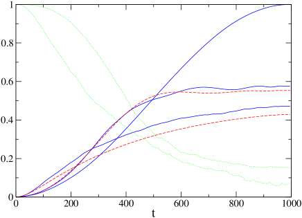
?figurename? 1: (Color online) Numerical solution of the quantum search algorithm using the exact Schrödinger equation (blue, solid curves) or the derived master equation (41) (red, dashed curves). We plot the probability of overlapping with the searched state. Blue (solid) curves are obtained, from top to bottom, for $\lambda=0$ , $\lambda=10^{-4}$ and $\lambda=5\times 10^{-4}$. For the two last cases, the corresponding approximated solution is also shown, also from top to bottom. Also for these two cases, green (dotted) curves show how decoherence manifests as time evolves, by plotting the magnitude defined in Eq. (43).

The results of our calculations are shown in Fig. 1. We plot the probability of overlapping with the searched stated during the evolution of the system. Solid (blue) lines are obtained from the exact solution to the Schrödinger equation. The upper curve corresponds to the case of no coupling to the environment ($\lambda=0)$ . Since the quantum computer runs during a ’Grover time’, the probability approaches unity. The two lower curves have been obtained, from top to bottom, for $\lambda=10^{-4}$ and $\lambda=5\times 10^{-4}$, giving $c_{1}=1.2,c_{2}=7.2\times 10^{-4}$ and $c_{1}=6,c_{2}=1.8\times 10^{-2}$, respectively. The interaction with the environment translates into a worse performance of the adiabatic search, which is manifested as a lower probability of success. This effect becomes stronger as the coupling to the bath increases. The degree of decoherence can be measured by several means. Here, as a figure of merit we calculate the magnitude Montina :

$$\mathbb{C}=\sqrt{2Tr(\rho_{S}^{2})-1},$$ (43)

which is also shown in the same figure for the same values of $\lambda$ . Clearly, the decoherence increases with time. This effect is more pronounced for a larger coupling, giving rise to an almost completely incoherent, and equally probable mixture, of the $\{|m>,|p>\}$ states.

One can also observe that the approximation obtained by solving the derived master equation (red, dashed curves) becomes more accurate for lower values of the coupling, in accordance to criteria Eq. (42). Indeed, most of the difference observed for the smallest $\lambda$ are due to oscillations , corresponding to the fact that the complete numerical solution has been obtained for a particular realization of the couplings in Eq. (31), while these constants have been averaged out in obtaining (41).

VI Conclusions

In this paper, we have first discussed the so-called Hilbert space Average Method, as an alternative to describe open quantum systems. We extended the method to the case of a system subject to a time-dependent Hamiltonian. We also made a connection of the evolution equations for this method with known master equations.

We next discussed a simple model which can be useful for the study of a quantum computer performing an adiabatic quantum search, while in contact with an environment. The ultimate purpose of such study is, of course, the understanding of the effects of decoherence on the performance of the computation. The model for the environment is simply a band of equally spaced levels with random coupling to the qubits of the quantum computer. In spite of its simplicity, we have shown that it incorporates decoherence effects in a clear way. The equations for the reduced system can be studied either under the form of HAM dynamics or master equations.

One can also, for this model, perform an exact numerical simulation of the total system (including the environment). We have performed such a numerical study, and compared the results with the approximated dynamics of the system. As expected, increasing the strength of the coupling between the system and the environment implies a larger degree of decoherence, which translates into a lower probability of success for the quantum search. On the other hand, increasing the coupling also means that the master equation gives a poorer description of the actual dynamics. The degree of approximation is controlled by the criteria derived for HAM equations within similar models for the environment.

Acknowledgments

I would like to acknowledge the comments made by M.C. Bañuls, I. de Vega and A. Romanelli, during interesting discussions, and also the hospitality of the Max-Planck-Institut für Quantenoptik in Munich. This work has been supported by the Spanish Ministerio de Educación y Ciencia through Projects AYA2007-67626-C03-C1 and FPA2005-00711.

- (1) M. Nielssen and I. Chuang, Quantum Computation and Quantum Information, Cambridge University Press, (2000).
- (2) M.H.S. Amin, P.J. Love and C.J.S. Truncik, Phys. Rev. Lett. 100, 060503 (2008).
- (3) A. Montina and F.T. Arecchi, Phys. Rev. Lett. 100, 120401 (2008).
- (4) W. Cui, Z.R. Xi and Y. Pan, Phys. Rev. A 77, 032117 (2008).
- (5) G. Gordon, G. Kurizki and D.A. Lidar, Phys. Rev. Lett. 101, 010403 (2008).
- (6) F. Verstraete, M.M. Wolf and J.I. Cirac, arXiv:quant-ph/0803.1447.
- (7) H. Ollivier, D. Poulin and W. H. Zurek, Phys. Rev. Lett. 93, 220401 (2004).
- (8) H.P. Breuer and F. Petruccione, The Theory of Open Quantum Systems (Oxford University Press, New York, 2007).
- (9) J. Gemmer, M. Michel, and G. Mahler. Quantum Thermodynamics: Emergence of Thermodynamic Behavior Within Composite Quantum Systems. Springer. Berlin, Heidelberg, New York (2004).
- (10) M. Michel, Nonequilibrium Aspects of Quantum Thermodynamics, dissertation Universität Stuttgart (2006), http://personal.ee.surrey.ac.uk/Personal/M.Michel/
- (11) H.P. Breuer, J. Gemmer and M. Michel, Phys. Rev. E 73, 016139 (2006).
- (12) L. K. Grover, in STOC’96, Proceedings of the 28thAnnual Symposium on Theory of Computing (ACM, New York, 1996), p. 212; L.K. Grover, Phys. Rev. Lett. 79, 325 (1997).
- (13) L. K. Grover, A.M. Sengupta, Phys. Rev. A 65, 032319 (2002), arXiv:quant-ph/0109123.
- (14) M. Boyer, G. Brassard, P. Høyer, and A. Tapp, Fortsch. Phys. 46 (1998) 493, arXiv:quant-ph/9605034.
- (15) E. Farhi, J. Goldstone, S. Gutmann and M. Sipser, arXiv:quant-ph/0001106.
- (16) E. Farhi, J. Goldstone, S. Gutmann and D. Nagaj, Int. J. Quantum Inf. 6, 503 (2008).
- (17) J. Roland and N. J. Cerf, Phys. Rev. A 65, 042308 (2002).
- (18) S. Das, R. Kobes and G. Kunstatter, J. Phys. A: Math. Gen. 36 (2003) 2839.
- (19) A. M. Childs, E. Farhi and J. Preskill, Phys. Rev. A 65, 012322 (2001).
- (20) M.S Sarandy and D.A.Lidar, Phys. Rev. A 71, 012331 (2005); Phys. Rev. Lett. 95, 250503 (2005).
- (21) S. Ashhab, J. R. Johansson and F. Nori, Phys. Rev. A 74, 052330 (2006).
- (22) J.Åberg, D. Kult, and E. Sjöqvist, Phys. Rev. A 71, 060312 (2005).
- (23) J.Åberg, D. Kult, and E. Sjöqvist, Phys. Rev. A 72, 042317 (2005).
- (24) M. Tiersch and R. Schützhold, Phys. Rev. A 75, 062313 (2007).
- (25) A. Pérez and A. Romanelli, Phys. Rev. A 76, 052318 (2007).
- (26) M. H. S. Amin, C. J. S. Truncik and D. V. Averin, arXiv:quant-ph/0803.1196.
- (27) J. Johansson, M.H.S. Amin, A.J. Berkley, P. Bunyk, V. Choi, R. Harris, M.W. Johnson, T.M. Lanting, Seth Lloyd and G. Rose, arXiv:cond-mat/0807.0797.
- (28) M. Suzuki. Phys. Lett. A 146, 319 (1990).