Dyadosphere formed in gravitational collapse

Abstract

We first recall the concept of Dyadosphere (electron-positron-photon plasma around a formed black holes) and its motivation, and recall on (i) the Dirac process: annihilation of electron-positron pairs to photons; (ii) the Breit-Wheeler process: production of electron-positron pairs by photons with the energy larger than electron-positron mass threshold; the Sauter-Euler-Heisenberg effective Lagrangian and rate for the process of electron-positron production in a constant electric field. We present a general formula for the pair-production rate in the semi-classical treatment of quantum mechanical tunneling. We also present in the Quantum Electro-Dynamics framework, the calculations of the Schwinger rate and effective Lagrangian for constant electromagnetic fields. We give a review on the electron-positron plasma oscillation in constant electric fields, and its interaction with photons leading to energy and number equipartition of photons, electrons and positrons. The possibility of creating an overcritical field in astrophysical condition is pointed out. We present the discussions and calculations on (i) energy extraction from gravitational collapse; (ii) the formation of Dyadosphere in gravitational collapsing process, and (iii) its hydrodynamical expansion in Reissner Nordström geometry. We calculate the spectrum and flux of photon radiation at the point of transparency, and make predictions for short Gamma-Ray Bursts.

1 Introduction

Motivations and Dyadosphere.   It is an one of most important issues in modern physics to understand how gravitational energy transforms to electromagnetic and rotational energies to during the process of gravitational collapses to black holes, in connection with observations. The primal steps toward the understanding of this issue are studies of electromagnetic properties of spinning and non-spinning black holes: (i) reversible and irreversible transformations – the Christodoulou-Ruffini formula, (ii) electron-positron pair-production in Kerr-Newmann geometry – the Damour-Ruffini proposal for Gamma Ray Bursts (GRBs), (iii) formation of electron-positron-photon plasma – Preparata-Ruffini-Xue Dyadopshere.

Pair-production.   The annihilation of electron-positron pair to two photons, and its inverse process – the production of electron-positron pair by the collision of two photons, as well as the electron-positron pair production from the vacuum in constant electromagnetic fields, were studied in quantum mechanics by Dirac, Breit, Wheeler, Sauter, Euler, Heisenberg respectively in 1930’s, and Schwinger in Quantum Electro-Dynamics (QED) in 1951.

Nonuniform fields.   It has been a difficult task to obtain the rate of electron-positron pair production in varying electromagnetic fields in space and time. This issue has attracted much attention not only for its theoretical viewpoint, but also its possible applications in heavy-ion collisions and high-energy laser beams, as well as astrophysics.

Plasma oscillation.   A naive expectation is that such external electric field rapidly vanishes for its source neutralized by electrons and positrons produced. However, the back reaction (screening effect) of electron-positron pairs on the external fields leads to the plasma oscillation phenomenon: electrons and positron oscillating back and forth in phase with alternating electric field. Beside electron-positron pairs oscillating together with the electric field, they interact with photons via the Dirac and Breit-Wheeler processes, and approach to a thermal configuration.

Critical fields on the surface of massive nuclear cores.   In ground based laboratories, it is rather difficult to built up electromagnetic fields at the order of the critical field value $E_{c}$ in macroscopic space-time scales. However, in the arena of astrophysics, supercritical electric fields are energetic-favorably developed on the surface of neutron star cores, due to strong, electroweak and gravitational interactions of degenerate nucleons and electrons.

Dyadosphere formed in gravitational collapse.   Initiating with supercritical electric fields on the surface, gravitational collapses of nuclear massive cores and processes of pair production, annihilation and oscillation lead to the formation of high energetic and dense plasma of electrons, positrons and photons, Dyadosphere that we proposed in 1998.

Hydrodynamic expansion after gravitational collapse.   The adiabatic and hydrodynamic expansion of the electron-positron-photon plasma after gravitational collapse, up to the transparency to photons, account for daily observing phenomena of Gamma Ray Bursts (GRBs).

Predications in connection with short Gamma ray Bursts.   Armed with a complete knowledge of all these fundamental processes, we present our understanding on the genuine origin of GRB-phenomenon, and make some predictions in connection with observations of short GRBs.

2 Basic motivations and Dyadosphere

Energetics of Electromagnetic Black Holes.

The process of gravitational collapse of a massive core generally leads to a black hole characterized by all the three fundamental parameters: the mass-energy $M$, the angular momentum $L$, and charge $Q$ rw . The phenomenon of gravitational collapse is crucial for the evolution of the system. Nonetheless in order not to involve its complex dynamics at this stage, we assume that the collapse has already occurred. Correspondingly a generally charged and rotating black hole has been formed whose curved space-time is described by the stationary Kerr-Newmann geometry in Boyer-Lindquist coordinates $(t,r,\theta,\phi)$

$$ds^{2} = {\frac{\Sigma}{\Delta}}dr^{2}+\Sigma d\theta^{2}+{\frac{\Delta}{\Sigma}}(dt-a\sin^{2}\theta d\phi)^{2}$$ (1)

$$+ {\frac{\sin^{2}\theta}{\Sigma}}\left[(r^{2}+a^{2})d\phi-adt\right]^{2},$$

where $\Delta=r^{2}-2Mr+a^{2}+Q^{2}$ and $\Sigma=r^{2}+a^{2}\cos^{2}\theta$, $a=L/M$ being the angular momentum per unit mass of the black hole. The Reissner-Nordström and Kerr geometries are particular cases for non-rotating $a=0$, and uncharged $Q=0$, black holes respectively. The total energy in terms of the Coulomb and rotational energies is described by the Christodoulou–Ruffini mass formula dr2

$$M^{2}c^{4}=\left(M_{\mathrm{ir}}c^{2}+{\frac{c^{2}Q^{2}}{4GM_{\mathrm{ir}}}}\right)^{2}+{\frac{L^{2}c^{8}}{4G^{2}M_{\mathrm{ir}}^{2}}},$$

$$\left({\frac{c^{2}}{16G^{2}M_{\mathrm{ir}}^{4}}}\right)\left(Q^{4}+4L^{2}c^{4}\right)\leq 1,$$ (2)

where $M_{\mathrm{ir}}$ is the irreducible mass. The reversible (irreducible) process of the black hole, characterized by constant (increasing) irreducible mass, can (cannot) be inverted bringing the black hole to its original state. Energy can be extracted approaching arbitrarily close to reversible processes which are the most efficient ones. Namely, from Eq. (2) it follows that up to 29$\%$ of the mass-energy of an extreme Kerr black hole ($M^{2}=a^{2}$) stored in its rotational energy term ${\frac{Lc^{4}}{2GM_{\mathrm{ir}}}}$, whereas up to 50$\%$ of the mass energy of an extreme EMBH with $(Q=M)$ stored in the electromagnetic energy term ${\frac{c^{2}Q^{2}}{4GM_{\mathrm{ir}}}}$, can be in principle extracted.

Vacuum polarization around an Electromagnetic Black Hole.

It was pointed dr that via Sauter, Heisenberg, Euler and Schwinger process, the electron-positron pair production occurring around an superritical Electromagnetic Black Hole (EMBH) is actually a very efficient almost reversible process of energy extraction, and extractable energy is up to $10^{54}$ergs that accounts for very energetic phenomenon of GRBs. In order to study the pair production in the Kerr-Newmann geometry, at each event $(t,r,\theta,\phi)$ a local Lorentz frame is introduced, associated with a stationary observer ${\mathcal{O}}$ at the event $(t,r,\theta,\phi)$. A convenient frame is defined by the following orthogonal tetrad

$${\bf\omega}^{(0)} = (\Delta/\Sigma)^{1/2}(dt-a\sin^{2}\theta d\phi),$$ (3)

$${\bf\omega}^{(1)} = (\Sigma/\Delta)^{1/2}dr,$$ (4)

$${\bf\omega}^{(2)} = \Sigma^{1/2}d\theta,$$ (5)

$${\bf\omega}^{(3)} = \sin\theta\Sigma^{-1/2}((r^{2}+a^{2})d\phi-adt).$$ (6)

In the so fixed Lorentz frame, the electric potential $A_{0}$, the electric field ${\bf E}$ and the magnetic field ${\bf B}$ are given by the following formulas,

$$A_{0}=\boldsymbol{\omega}_{a}^{(0)}A^{a},\quad{\bf E}^{\alpha}=\boldsymbol{\omega}_{\beta}^{(0)}F^{\alpha\beta},\quad{\bf B}^{\beta}={\frac{1}{2}}\boldsymbol{\omega}_{\gamma}^{(0)}\epsilon^{\alpha\gamma\delta\beta}F_{\gamma\delta}.$$ (7)

One then obtains $A_{0}=-Qr(\Sigma\Delta)^{-1/2}$, while the electromagnetic fields ${\bf E}$ and ${\bf B}$ are parallel to the direction of $\boldsymbol{\omega}^{(1)}$

$$E_{(1)} = Q\Sigma^{-2}(r^{2}-a^{2}\cos^{2}\theta),$$ (8)

$$B_{(1)} = Q\Sigma^{-2}2ar\cos\theta,$$ (9)

respectively. The spatial variation scale $GM/c^{2}$ of these background fields is much larger than the Compton wavelength $\hbar/m_{e}c$ of the quantum field, then, for what concern pair production, it is possible to consider the electric and magnetic fields defined by Eqs. (8,9) as constants in a neighborhood of a few wavelengths around any events $(r,\theta,\phi,t)$. Based on the equivalence principle, the rate of pair-production process in a constant field over a flat space-time can be locally applied to the case of the curved Kerr-Newmann geometry:

$${\frac{dN}{\sqrt{-g}d^{4}x}} = {\frac{e^{2}E_{(1)}B_{(1)}}{4\pi^{2}}}\sum_{n=1}^{\infty}{\frac{1}{n}}\coth\left({\frac{n\pi B_{(1)}}{E_{(1)}}}\right)$$ (10)

$$\cdot \exp\left(-{\frac{n\pi E_{\mathrm{c}}}{E_{(1)}}}\right),$$

where the critical field $E_{c}=m_{e}^{2}c^{3}/e\hbar$. It was assumed that electron and positron produced fly apart from each other, one goes inward to neutralize EMBHs and another goes to infinity. This view was fundamentally modified in Refs. prx98 ; rjapan ; prxprl by the novel concept of the Dyadosphere.

Dyadosphere: electron-positron-photon plasma.

We start with the Reissner-Nordström black holes and consider a spherical shell of proper thickness $\delta={\frac{\hbar}{mc}}\ll{\frac{MG}{c^{2}}}$ centered on the EMBH, the electric field is approximately constant in it. We can then at each value of the radius $r$ model the electric field as created by a capacitor of width $\delta$ and surface charge density $\sigma(r)={\frac{Q}{4\pi r^{2}}}$, and express Eq. (10) as,

$${\frac{dN}{\sqrt{-g}d^{4}x}}={\frac{1}{4\pi c}}\left({\frac{eE}{\pi\hbar}}\right)^{2}e^{-{\frac{\pi E_{\mathrm{c}}}{E}}}={\frac{1}{4\pi c}}\left({\frac{4e\sigma}{\hbar}}\right)^{2}e^{-{\frac{\pi\sigma_{\mathrm{c}}}{\sigma}}},$$ (11)

where electric field $E=4\pi\sigma$, $\sigma_{\mathrm{c}}={\frac{1}{4\pi}}E_{\mathrm{c}}$ is the critical surface charge density. The pair creation process in these shells will continue until a value of the surface charge density reaches the critical value $\sigma_{\mathrm{c}}$, and it takes

$$\Delta\tau = {\frac{\sigma-\sigma_{\mathrm{c}}}{{\frac{e}{4\pi c}}\left({\frac{4e\sigma}{\hbar}}\right)^{2}e^{-{\frac{\pi\sigma_{\mathrm{c}}}{\sigma}}}\left({\frac{\hbar}{mc}}\right)}}\lesssim 1.99\left({\frac{\hbar}{mc^{2}\alpha}}\right)$$ (12)

$$= 1.76\cdot 10^{-19}\mathrm{s}.$$

This time is so short that the light travel time is smaller or approximately equal to the width $\delta$. Under these circumstances the correlation between shells can be approximately neglected, thus we can justify the approximation of describing the pair creation process shell by shell.

The Dyadosphere is composed by these shells from the horizon $r_{+}$ to $r_{ds}$, which is given by $E(r_{ds})=E_{c}$ and can be expressed as,

$$r_{\mathrm{ds}} = \left({\frac{\hbar}{mc}}\right)^{\frac{1}{2}}\left({\frac{GM}{c^{2}}}\right)^{\frac{1}{2}}\left({\frac{m_{\mathrm{p}}}{m}}\right)^{\frac{1}{2}}\left({\frac{e}{q_{\mathrm{p}}}}\right)^{\frac{1}{2}}$$ (13)

$$\cdot \left({\frac{Q}{\sqrt{G}M}}\right)^{\frac{1}{2}}\gg{\frac{GM}{c^{2}}},$$

using the Planck charge $q_{\mathrm{p}}=(\hbar c)^{1/2}$ and the Planck mass $m_{\mathrm{p}}=(\hbar c/G)^{1/2}$, which clearly shows the hybrid gravitational and quantum nature of this quantity. The total number of shells is about $(r_{ds}-r_{+})/{\frac{\hbar}{mc}}$ and the total number of pairs,

$$N_{e^{+}e^{-}}\simeq{\frac{Q-Q_{\mathrm{c}}}{e}}\left[1+{\frac{(r_{ds}-r_{+})}{{\frac{\hbar}{mc}}}}\right].$$ (14)

We calculate the number and energy densities of pairs in the Dyadosphere

$$\!\!\!\!n_{e^{+}e^{-}}(r) = {\frac{Q}{e4\pi r^{2}\left({\frac{\hbar}{mc}}\right)}}\left[1-\left({\frac{r}{r_{ds}}}\right)^{2}\right],$$

$$\epsilon_{e^{+}e^{-}}(r) = {\frac{Q^{2}}{8\pi r^{4}}}\left[1-\left({\frac{r}{r_{ds}}}\right)^{4}\right],$$ (15)

as shown in Figs. 1,

Figure 1: The number-density $n_{e^{+}e^{-}}(r)$ (left) and average energy per pair in MeV (right) are plotted as a function of the radial coordinate for $\mu=M/M_{\odot}=10$ and $\xi=Q/M=1$ (upper curve) and $\xi=0.1$ (lower curve).

and total energy is then

$$E_{e^{+}e^{-}}^{\mathrm{tot}}={\frac{1}{2}}{\frac{Q^{2}}{r_{+}}}\left(1-{\frac{r_{+}}{r_{\mathrm{ds}}}}\right)\left[1-\left({\frac{r_{+}}{r_{\mathrm{ds}}}}\right)^{2}\right].$$ (16)

Due to the very large pair density given by Eq. (15) and to the sizes of the cross-sections for the process $e^{+}e^{-}\leftrightarrow\gamma+\gamma$, the system is expected to thermalize to a plasma configuration for which

$$N_{e^{+}}=N_{e^{-}}=N_{\gamma}=N_{e^{+}e^{-}},\quad T_{\circ}={\frac{E^{\mathrm{tot}}_{e^{+}e^{-}}}{3N_{e^{+}e^{-}}\cdot 2.7}}.$$ (17)

In Fig. 2, the total energy (16) and the average energy per pair ${\frac{E^{\mathrm{tot}}_{e^{+}e^{-}}}{N_{e^{+}e^{-}}}}$ are shown in terms of EMBH’s mass $\mu$ and charge $\xi$.

Figure 2: Left: Total energy of Dyadosphere as a function of EMBHs’ mass and charge parameters $\mu,\xi$. Right: The average energy per pair is shown here as a function of the EMBH mass in solar mass units for $\xi=1$ (solid line), $\xi=0.5$ (dashed line) and $\xi=0.1$ (dashed and dotted line).

Recently, the Dyadotorus: the plasma of electron-positron-photon created in Kerr-Newmann black holes is studied cgrr2007 .

3 Production of electron-positron pairs

Early quantum electrodynamics.

We recall three results, which played a crucial role in the development of the Quantum Electro-Dynamics (QED). The first is the Dirac process of an electron-positron pair annihilation into two photons,

$$e^{+}+e^{-}\rightarrow\gamma_{1}+\gamma_{2},$$ (18)

and the cross-section in the rest frame of electron:

$$\sigma_{e^{+}e^{-}}\simeq\frac{\pi}{\gamma}\left(\frac{\alpha\hbar}{m_{e}\,c}\right)^{2}\left[\ln\left(2\gamma\right)-1\right];$$ (19)

where $\gamma\equiv{\mathcal{E}_{+}}/m_{e}\,c^{2}\gg 1$ is the energy of the positron and $\alpha=e^{2}/(4\pi\hbar c)$ is the fine structure constant. The second is the Breit-Wheeler process of electron-positron pair production by two photons collision,

$$\gamma_{1}+\gamma_{2}\rightarrow e^{+}+e^{-},$$ (20)

which is the inverse Dirac-process (18) and the cross-section is related to (18) by the ${\mathcal{C}PT}$-theorem ,

$$\sigma_{\gamma\gamma}=2\beta^{2}\sigma_{e^{+}e^{-}},$$ (21)

where $\beta$ is the relative velocity of electron and positron. The third is the vacuum polarization in external uniform electromagnetic field, studied by Heisenberg and Euler, following Sauter’s work on quantum tunneling probability from negative energy states [see Fig. (3)],

$$|T|^{2} = \frac{|{\rm transmission\hskip 5.69046ptflux}|}{|{\rm incident\hskip 5.69046ptflux}|}\sim e^{-\pi\frac{m_{e}^{2}c^{3}}{\hbar eE}},$$ (22)

$$E_{c} \equiv \frac{m_{e}^{2}c^{3}}{e\hbar},\quad{\rm critical-field},$$

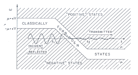
Figure 3: In presence of a strong enough electric field the boundaries of the classically allowed states (“positive” or “negative”) can be so tilted that a “negative” is at the same level as a “positive” (level crossing). Therefore a “negative” wave-packet from the left will be partially transmitted, after an exponential damping due to the tunneling through the classically forbidden states, as s “positive” wave-packet outgoing to the right. $\mu$ is particle’s mass, $\epsilon V$ potential energy and $\omega$ energy.

$E_{c}\simeq 1.3\cdot 10^{16}\,{\rm V/cm}$, $10^{6}$ larger than the value required to ionize a hydrogen atom. Heisenberg and Euler obtained nonlinear Lagrangian from the Dirac theory,

$$\Delta{\mathcal{L}}_{\rm eff} = \frac{e^{2}}{16\pi^{2}\hbar c}\int^{\infty}_{0}e^{-s}\frac{ds}{s^{3}}$$

$$\cdot \Big{[}is^{2}\,\bar{E}\bar{B}\frac{\cos(s[\bar{E}^{2}-\bar{B}^{2}+2i(\bar{E}\bar{B})]^{1/2})+{\rm c.c.}}{\cos(s[\bar{E}^{2}-\bar{B}^{2}+2i(\bar{E}\bar{B})]^{1/2})-{\rm c.c.}}$$

$$+ \left(\frac{m_{e}^{2}c^{3}}{e\hbar}\right)^{2}+\frac{s^{2}}{3}(|\bar{B}|^{2}-|\bar{E}|^{2})\Big{]};$$

$$\bar{E} = |{\bf E}|/E_{c},\quad\bar{B}=|{\bf B}|/E_{c},$$ (23)

and its series expansion in powers of $\alpha$,

$$\Delta{\mathcal{L}}_{\rm eff} =\frac{2\alpha^{2}}{45m_{e}^{4}}\left\{({\bf E}^{2}\!-\!{\bf B}^{2})^{2}+7({\bf E}\cdot{\bf B})^{2}\right\}+\cdot\cdot\cdot.$$ (24)

They found facts that $\Delta{\mathcal{L}}_{\rm eff}$ is a complex function of ${\bf E}$ and ${\bf B}$, the imaginary part is associated with pair production when the electric field $E\gtrsim E_{c}$, and the vacuum behaves as a dielectric and permeable medium in which,

$$D_{i}=\sum_{k}\epsilon_{ik}E_{k},\hskip 14.22636ptH_{i}=\sum_{k}\mu_{ik}B_{k},$$ (25)

where complex $\epsilon_{ik}$ and $\mu_{ik}$ are the field-dependent dielectric and permeability tensors of the vacuum.

Quantum electrodynamics.

The QED-Lagrangian describing the interacting system of photons, electrons, and positrons reads

$${\mathcal{L}} = {\mathcal{L}}_{0}^{e^{+}e^{-}\gamma}(\bar{\psi},\psi,A_{\mu})+{\mathcal{L}}_{\rm int}(\bar{\psi},\psi,A_{\mu}),$$ (26)

where ${\mathcal{L}}_{0}^{e^{+}e^{-}\gamma}$ is for free electrons, positron and photons. An external field $A^{\rm e}_{\mu}$ is incorporated by adding to the quantum field $A_{\mu}$ in

$${\mathcal{L}}_{\rm int}+{\mathcal{L}}^{\rm e}_{\rm int}=-e\bar{\psi}(x)\gamma^{\mu}\psi(x)\left[A_{\mu}(x)+A^{\rm e}_{\mu}(x)\right].$$ (27)

The amplitude for the vacuum to vacuum transition in the presence of$A^{\rm e}$:

$$\langle 0|0\rangle \!\!\!\!\!\!=\!\!\!\!\!\! \frac{Z[A^{\rm e}]}{Z[0]},$$

$$Z[A^{\rm e}] \!\!\!\!\!\!=\!\!\!\!\!\! \int[{\mathcal{D}}\psi{\mathcal{D}}\bar{\psi}{\mathcal{D}}A_{\mu}]\exp\left[i\int d^{4}x({\mathcal{L}}+{\mathcal{L}}^{\rm e}_{\rm int})\right].$$ (28)

The effective action as a functional of $A^{\rm e}$ is:

$$\Delta{\mathcal{A}}_{\rm eff}[A^{\rm e}]\equiv-i\ln\langle 0|0\rangle.$$ (29)

Under the assumption that $A^{\rm e}(x)$ varies smoothly over a finite spacetime region, we may define an approximately local effective Lagrangian $\Delta{\mathcal{L}}_{\rm eff}[A^{\rm e}(x)]$,

$$\Delta{\mathcal{A}}_{\rm eff}[A^{\rm e}]\simeq\int d^{4}x\Delta{\mathcal{L}}_{\rm eff}[A^{\rm e}(x)]\approx V\Delta t\Delta{\mathcal{L}}_{\rm eff}[A^{\rm e}],$$ (30)

where $V$ is the spatial volume and time interval $\Delta t$, over which the field is nonzero. The amplitude of the vacuum to vacuum transition (28) has the form,

$$\langle 0|0\rangle=e^{-i(\Delta{\mathcal{E}}_{0}-i\Gamma/2)\Delta t},$$ (31)

where vacuum-energy difference $\Delta{\mathcal{E}}_{0}={\mathcal{E}}_{0}(A^{\rm e})-{\mathcal{E}}_{0}(0)$, and $\Gamma$ is the vacuum decay rate. The probability that the vacuum remains as it is in the presence of the external field $A^{\rm e}$ is

$$|\langle 0|0\rangle|^{2}=e^{-2{\rm Im}\Delta{\mathcal{A}}_{\rm eff}[A^{\rm e}]}.$$ (32)

This determines the decay rate of the vacuum caused by the production of electron and positron pairs:

$$\frac{\Gamma}{V}=\frac{2{\rm\,Im}\Delta{\mathcal{A}}_{\rm eff}[A^{\rm e}]}{\Delta tV}\approx 2{\rm\,Im}\Delta{\mathcal{L}}_{\rm eff}[A^{\rm e}];$$ (33)

and vacuum-energy variation

$$\frac{\Delta{\mathcal{E}}_{0}}{V}=-\frac{{\rm\,Re}\Delta{\mathcal{A}}_{\rm eff}[A^{\rm e}]}{\Delta tV}\approx-{\rm\,Re}\Delta{\mathcal{L}}_{\rm eff}[A^{\rm e}].$$ (34)

We calculate the imaginary part (33) and reproduce the Schwinger formula,

$$\frac{\Gamma}{V}=\frac{\alpha\varepsilon^{2}}{\pi^{2}}\sum_{n=1}\frac{1}{n^{2}}\frac{n\pi\beta/\varepsilon}{\tanh{n\pi\beta/\varepsilon}}\exp\left(-\frac{n\pi E_{c}}{\varepsilon}\right),$$ (35)

where $\varepsilon^{2}-\beta^{2}\equiv{\bf E}^{2}-{\bf B}^{2}$ and $\varepsilon\beta\equiv{\bf E}\,{\bf B}$. In addition, we calculate hagen1 ; rvxreport the real part (34),

$${\rm Re}(\Delta{\mathcal{L}}_{\rm eff}) = \frac{1}{2(2\pi)^{2}}\sum_{n,m=-\infty}^{\infty}{\!\!\!}^{\prime}\frac{1}{\tau^{2}_{m}+\tau^{2}_{n}}$$ (36)

$$\cdot \Big{[}\bar{\delta}_{m0}J(i\tau_{m}m^{2}_{e})-\bar{\delta}_{n0}J(\tau_{n}m^{2}_{e})\Big{]},$$

where $\tau_{n}=n\pi/e\varepsilon$, $\tau_{m}=m\pi/e\beta$,

$$J(z)=-\frac{1}{2}\Big{[}e^{-z}{\rm Ei}(z)+e^{z}{\rm Ei}(-z)\Big{]},$$ (37)

and ${\rm Ei}(z)$ is the exponential-integral function. In the weak-field expansion, we obtain Eq. (24). In the strong-field expansion, we obtain,

$${\rm Re}(\Delta{\mathcal{L}}_{\rm eff}) = \frac{1}{2(2\pi)^{2}}\sum_{n,m=-\infty}^{\infty^{\prime}}\frac{1}{\tau^{2}_{m}+\tau^{2}_{n}}$$

$$\cdot \Big{[}\bar{\delta}_{n0}\ln(\tau_{n}m^{2}_{e})-\bar{\delta}_{m0}\ln(\tau_{m}m^{2}_{e})\Big{]}+\cdot\cdot\cdot.$$

In the case $E\gg 1$, $B=0$ and $m=0$, we obtain,

$$(\Delta{\mathcal{L}}_{\rm eff}) = \frac{1}{2(2\pi)^{2}}\sum_{n=1}^{\infty}\frac{1}{\tau^{2}_{n}}\ln(\tau_{n}m^{2}_{e})+\cdot\cdot\cdot$$ (39)

$$= \frac{e^{2}E^{2}}{8\pi^{4}}\sum_{n=1}^{\infty}\frac{1}{n^{2}}\ln\left(\frac{n\pi E_{c}}{E}\right)+\cdot\cdot\cdot.$$

In the case $B\gg 1$, $E=0$ and $n=0$, we obtain,

$$(\Delta{\mathcal{L}}_{\rm eff}) = -\frac{1}{2(2\pi)^{2}}\sum_{m=1}^{\infty}\frac{1}{\tau^{2}_{m}}\ln(\tau_{m}m^{2}_{e})+\cdot\cdot\cdot$$ (40)

$$= -\frac{e^{2}B^{2}}{8\pi^{4}}\sum_{m=1}^{\infty}\frac{1}{m^{2}}\ln\left(\frac{m\pi E_{c}}{B}\right)+\cdot\cdot\cdot.$$

Nonuniform electric fields.

Let the field vector ${\bf E}(z)$ point in the $\hat{\bf z}$-direction. The one-dimensional electric potential $A_{0}(z)=-\int^{z}dz^{\prime}E(z^{\prime})$ and the positive and negative continuum energy-spectra are

$${\mathcal{E}}_{\pm}=\pm\sqrt{(cp_{z})^{2}+c^{2}{\bf p}_{\perp}^{2}+(m_{e}c^{2})^{2}}+V(z),$$ (41)

where $p_{z}$ is the classical momentum in $\hat{\bf z}$-direction, ${\bf p}_{\perp}$ transverse momenta, and $V(z)=eA_{0}(z)$ potential energy. The crossing energy-levels between two energy-spectra ${\mathcal{E}}_{\pm}$ (41) appear, $\epsilon\equiv{\mathcal{E}}_{+}={\mathcal{E}}_{-}$. The probability amplitude for quantum tunneling process can be estimated by a semi-classical calculation using WKB method (see e.g. krx2007 ):

$$W_{\rm WKB}(|{\bf p}_{\perp}|,\epsilon) \equiv \exp\left\{-{\frac{2}{\hbar}}\int_{z_{-}}^{z_{+}}\kappa_{z}dz\right\},$$ (42)

where $\kappa=-ip_{z}$ and the turning points $z_{\pm}$ determined by setting $p_{z}=0$

$$V[z_{\pm}]=\mp\big{[}c^{2}{\bf p}_{\perp}^{2}+m_{e}^{2}c^{4}\big{]}^{1/2}+\epsilon.$$ (43)

Changing the variable of integration from $z$ to $y(z)$,

$$y(z)=\frac{\epsilon-V(z)}{c{\sqrt{{\bf p}_{\perp}^{2}+m_{e}^{2}c^{2}}}},$$ (44)

we obtain $y_{-}(z_{-})=-1,y_{+}(z_{+})=+1$ and

$$W_{\rm WKB}(|{\bf p}_{\perp}|,\epsilon) = \exp\Big{[}-\frac{2E_{c}}{E_{0}}\left(1+\frac{{\bf p}_{\perp}^{2}}{m_{e}^{2}c^{2}}\right)$$ (45)

$$\cdot \int^{1}_{-1}dy\frac{\sqrt{1-y^{2}}}{\bar{E}(y)}\Big{]},$$

where $\bar{E}(y)=E[z(y)]/E_{0}$ and $z(y)$ is the inverse function of Eq. (44). The flux density of virtual particles attempt for tunneling at $z_{-}$ is

$$d^{3}J_{z}=v_{z}D_{s}\frac{d^{2}{\bf p}_{\perp}dp_{z}}{(2\pi\hbar)^{3}},\quad v_{z}=\partial\epsilon/\partial p_{z},$$ (46)

and the energy-variation $d\epsilon=|eE(z_{-})|dz$. Using Eqs. (45,46) and expanding up to ${\bf p}_{\perp}^{2}/(m_{e}^{2}c^{2})$, we obtain the WKB-rate of pair production per unit volume at given crossing energy-level $\epsilon(z_{-})$ is

$$\frac{\Gamma_{\rm WKB}[\epsilon(z_{-}),z_{-}]}{V} = D_{s}|eE(z_{-})|\int\frac{d^{2}{\bf p}_{\perp}}{(2\pi\hbar)^{3}}$$

$$\cdot e^{-{\pi c(G/2+g)}{{\bf p}_{\perp}^{2}/|eE_{0}|\hbar}}e^{-{\pi G}{E_{c}/E_{0}}}\!$$

$$\simeq D_{s}\frac{\alpha E_{0}E(z_{-})}{2\pi^{2}\hbar(G/2+g)}e^{-{\pi GE_{c}/E_{0}}},$$

where $V\equiv V_{\perp}dz,V_{\perp}=\int dxdy$; $D_{s}=2$ for a spin-$1/2$ particle and $D_{s}=1$ for spin-$0$. The $G$ and $g$ functions are

$$G[\epsilon(z_{-})] = \frac{2}{\pi}\int^{1}_{-1}dy\frac{\sqrt{1-y^{2}}}{\bar{E}(y)},$$

$$g[\epsilon(z_{-})] = \frac{1}{\pi}\int^{1}_{-1}\frac{y^{2}}{\sqrt{1-y^{2}}}\frac{dy}{\bar{E}(y)}.$$ (48)

Eq. (3) gives the semi-classical WKB-rate of pair-production per unit volume for any one-dimensional electric field ${\bf E}(z)$ and potential $V(z)$ krx2007 , provided crossing energy-levels $\epsilon$ between negative and positive energy-spectrum occur.

We apply our formula (3,48) to a uniform field case, obtain $G=1,g=G/2$,

$$\frac{\Gamma_{\rm WKB}}{V_{\perp}\Delta z}\simeq D_{s}\frac{\alpha E^{2}}{2\pi^{2}\hbar}e^{-{\pi E_{c}/E}},$$ (49)

which is independent of crossing energy-levels $\epsilon$ and coordinate $z$. gives the Sauter factor (22) and Heisenberg-Euler prefactor obtained from (23).

Sauter electric field.

As an example, we consider the nonuniform Sauter electric field localized within finite slice of space of width $\ell$ in the $xy$-plane krx2007 . Electric field ${\bf E}=E(z)\hat{\bf z}$ and potential energy $V(z)$ are given by

$$E(z) = E_{0}/{\rm cosh}^{2}\left({z}/{\ell}\right),$$ (50)

$$V(z) = \sigma\,m_{e}c^{2}\tanh\left({z}/{\ell}\right),$$ (51)

where

$$\sigma\equiv|eE_{0}|\ell/m_{e}c^{2}=(\ell/\lambda_{C})(E_{0}/E_{c})=\ell|eE_{0}|/m_{e}c^{2},$$ (52)

and see Fig. 4.

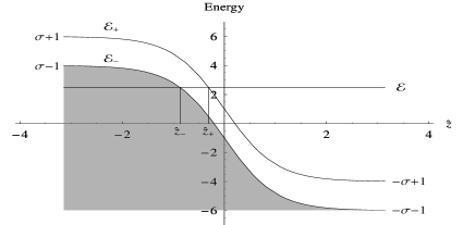
Figure 4: Positive and negative energy-spectra ${\mathcal{E}}_{\pm}(z)$ of Eq. (41) in units of $m_{e}c^{2}$, with $p_{z}=p_{\perp}=0$ as a function of $x=z/\ell$ for the Sauter potential $V_{\pm}(z)$ (51) for $\sigma=5$.

Using our formula (3,48) and integrating over $\epsilon(z_{-})$, we approximately obtain

$$\frac{\Gamma_{\rm WKB}}{V_{\perp}\ell}\simeq D_{s}\frac{e^{2}E^{2}_{0}}{8\pi^{3}\hbar}\sqrt{\frac{E_{0}}{E_{c}}}\frac{(\sigma^{2}-1)^{5/4}}{\sigma^{5/2}}e^{-{\pi G(0)E_{c}/E_{0}}}.$$ (53)

The comparison between pair-production rates in unbound uniform and bound nonuniform fields is given by the ratio $R_{\rm rate}$ of Eq. (49) and Eq. (53)

$$R_{\rm rate}=\sqrt{\frac{E_{0}}{E_{c}}}e^{{\pi E_{c}/E_{0}}}\frac{(\sigma^{2}-1)^{5/4}}{\sigma^{5/2}}e^{-{\pi G(0)E_{c}/E_{0}}}.$$ (54)

In Fig. (5), it is shown that the pair-production rate in the Sauter field becomes smaller as the confining size of the field becomes smaller.

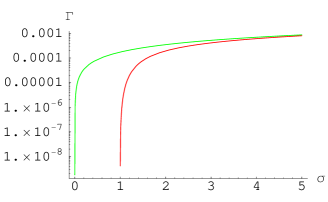
Figure 5: For $E_{0}=E_{c}$, $\sigma=\ell/\lambda_{C}$ (52) is the spatial size where electric field $E\not=0$. The ratio $R_{\rm rate}$ (54) is plotted as function of $\sigma$ in the left figure. The number of pairs created in Compton area and time as functions of $\sigma$ (up curve for Schwinger constant field (49) and low one is nonuniform Sauter field (53)) in the right figure.

In Ref. krx2007 , we present detailed calculations and discussions of pair-productions rate in various cases of nonuniform electric fields: the Sauter and Coulomb fields, as well as fields $E(z)\sim z$ and $E(z)\not=0,z>0$.

4 Plasma oscillations of electron-positron pairs in electric fields

We have discussed the Sauter-Heisenberg-Euler-Schwinger process for electron-positron pair production. However, we neglect the following dynamics:

1. the back reaction of pair production on the external electric field;

2. the screening effect of pairs on the external electric field strengths;

3. the motion of pairs and their interactions.

When these dynamics are considered, a phenomenon of electron-positron oscillation, plasma oscillation, takes place. We quantitatively discuss this phenomenon by using the relativistic Boltzmann-Vlasov equations RVX03d

$$\partial_{t}f_{e}+e\mathbf{E\cdot\nabla}_{\mathbf{p}}f_{e} =\mathcal{S}\left(\mathbf{E},\mathbf{p}\right)-\mathcal{C}_{e}\left(t,\mathbf{p}\right),$$ (55)

$$\partial_{t}f_{\gamma} =2\mathcal{C}_{\gamma}\left(t,\mathbf{k}\right),$$ (56)

where $f_{e}(f_{\gamma})$ is spatially independent distribution function of electrons (photons) in phase space; and the homogeneous Maxwell equations,

$$\partial_{t}\mathbf{E}=-\mathbf{j}_{p}\left(\mathbf{E}\right)-\mathbf{j}_{c}\left(t\right),$$ (57)

where $\mathbf{j}_{p}$ is the polarization current and $\mathbf{j}_{c}$ conduction current. The terms $\mathcal{C}_{e}\left(t,\mathbf{p}\right)$ and $\mathcal{C}_{\gamma}\left(t,\mathbf{k}\right)$ stand for collisions between electrons, positrons and photons. $\mathcal{S}\left(\mathbf{E},\mathbf{p}\right)$ is related to the pair-production rate (49),

$$\mathcal{S}\left(\mathbf{E},\mathbf{p}\right)=[1\pm 2f_{e}]\left(\frac{\Gamma}{V}\right)\delta^{3}({\bf p}),$$ (58)

where $[1\pm 2f_{e}]$ accounts for the Bose enhancement(+) and Pauli blocking (-).

These Equations (55-57) are integrated with the following initial conditions of $|{\bf E}|=E_{0}=9E_{c}$ and null densities of electrons, positron and photons. The results of the numerical integration in units of the Compton time $\tau_{C}$ and length $\lambda_{C}$ are shown in Fig. 6: at early times,

1. the electric field does not abruptly reach the equilibrium value but rather oscillates with decreasing amplitude;

2. electrons and positrons oscillates in the electric field direction, reaching ultra relativistic velocities;

3. the role of the $e^{+}e^{-}\rightleftarrows$ $\gamma\gamma$ scatterings is marginal in the early time of the evolution.

At late times the system is expected to relax to a plasma configuration of thermal equipartition with the asymptotic behavior:

1. the electric field is screened to about the critical value: $E\simeq E_{\mathrm{c}}$ for $t\sim 10^{3}-10^{4}\tau_{\mathrm{C}}\gg\tau_{\mathrm{C}}$;

2. the initial electromagnetic energy density is distributed over electron–positron pairs and photons, indicating energy equipartition;

3. photons and electron–positron pairs number densities are asymptotically comparable, indicating number equipartition.

Note that we show rvx2007 that such phenomenon of plasma oscillation occurs not only for strong fields, but also for weak fields, in addition, a detailed study of thermalization of electrons–positrons–photons plasma is given in Ref. arv2007 . The thermalized plasma starts hydrodynamical expansion described by hydrodynamic equations RVX03c ; RSWX00 ; rswx1999 .

Figure 6: In left figure: We plot for $t<150\tau_{\mathrm{C}}$, from the top to the bottom panel: a) electromagnetic field strength; b) electrons energy density; c) electrons number density; d) photons energy density; e) photons number density as functions of time. The right figure: We plot for $t<7000\tau_{\mathrm{C}}$ as the same quantities as in left.

5 Super critical field on the surface of massive nuclear cores

Electromagnetic properties of massive nuclear cores

Based on numerical rrx2006 and analytical rrx2007 ; rrxmg2007 approaches to the relativistic Thomas-Fermi theory, we study electron configurations and electromagnetic properties of massive nuclear cores of mass number $A$ and radius $R_{c}$

$$A \!\!\!\!\simeq\!\!\!\! \left(\frac{M_{\rm Planck}}{m_{N}}\right)^{3}\!\!\!\sim\!\!\!10^{57},\!\!\!\quad\!\!\!R_{c}\!\!\!\simeq\!\!\!\frac{\hbar}{m_{\pi}c}N_{p}^{1/3}\!\!\!\sim\!\!\!10{\rm km},$$ (59)

where $M_{\rm Planck},m_{N},m_{\pi}$ are Planck, nucleon and pion masses, with the global neutrality condition: the same proton and electron numbers $N_{p}=N_{e}$. We show that close to core surface, it exists supercritical electric field $E>E_{c}$, prove that this configuration is stable and energetically favorable against the configuration with the local neutrality condition: the same proton and electron densities $n_{e}(x)=n_{p}(x)$, usually adopted.

The Thomas-Fermi theory for the electrostatic equilibrium of electron distributions $n_{e}(r)$ around extended nuclear cores can be described as follow. Degenerate electron density $n_{e}(r)$, Fermi momentum $P_{e}^{F}$ and Fermi-energy ${\mathcal{E}}_{e}(P_{e}^{F})$ are related by

$$n_{e}(r) = \frac{(P_{e}^{F})^{3}}{3\pi^{2}\hbar^{3}},$$ (60)

$$\quad{\mathcal{E}}_{e}(P_{e}^{F}) \!=\! [(P_{e}^{F}c)^{2}+m_{e}^{2}c^{4}]^{1/2}\!-\!m_{e}c^{2}\!-\!V_{\rm coul}(r),$$

where $V_{\rm coul}(r)$ is Coulomb potential energy. The electrostatic equilibrium of electron distributions is determined by

$${\mathcal{E}}_{e}(P_{e}^{F})=0,$$ (61)

which means the balance of electron’s kinetic and potential energies in Eq. (60) and degenerate electrons occupy energy-levels up to $+m_{e}c^{2}$. Eqs. (60,61) give:

$$n_{e}(r) = \frac{1}{3\pi^{2}(c\hbar)^{3}}\left[V^{2}_{\rm coul}(r)+2m_{e}c^{2}V_{\rm coul}(r)\right]^{3/2}.$$ (62)

The Gauss law leads the following Poisson equation and boundary conditions,

$$\Delta V_{\rm coul}(r) = 4\pi\alpha\left[n_{p}(r)-n_{e}(r)\right];$$

$$V_{\rm coul}(\infty) = 0,\quad V_{\rm coul}(0)={\rm finite}.$$ (63)

Degenerate proton and densities $n_{p,n}(r)$ are constants inside core $r\leq R_{c}$ and vanishes outside the core $r>R_{c}$.

$$\!\!\!\!\!\!\!\!\!n_{p,n}(r) = \frac{(P_{p,n}^{F})^{3}}{3\pi^{2}\hbar^{3}},$$ (64)

$${\mathcal{E}}_{p,n}(P_{e}^{F}) \!=\! [(P_{p,n}^{F}c)^{2}\!+\!m_{p,n}^{2}c^{4}]^{1/2}\!-\!m_{p,n}c^{2}\!+\!V_{\rm coul}(r)\delta_{p},$$

where $P_{p,n}^{F},{\mathcal{E}}_{p,n}(P_{e}^{F})$ are Fermi momenta, energies of protons and neutrons, and $\delta_{p}$ indicates $V_{\rm coul}(r)$ for protons only. Neutrinos assumed to escape from massive cores, the energetic equation for the $\beta-$equilibrium of neutrons, protons and electrons is

$${\mathcal{E}}_{n}(P_{n}^{F})={\mathcal{E}}_{p}(P_{p}^{F})+{\mathcal{E}}_{e}(P_{e}^{F}),$$ (65)

which gives the relationship between the neutron, proton and mass numbers $N_{n},N_{p},A=N_{n}+N_{p}$. We integrate these equations are integrated and show results in Fig. (7)

Figure 7: Potential energy $-V_{\rm coul}(r)$ (left) and electric field $E(r)\sim-V^{\prime}_{\rm coul}(r)$ (right) are plotted as a function of $(r-R_{c})/(10\lambda_{\pi})$.

The configuration is electrostatic stable, since the mean repulsive energy is much smaller than mean gravitational binding $0.1M_{N}c^{2}$ for protons in the surface layer.

6 Geometry of gravitationally collapsing cores

The Tolman-Oppenheimer-Snyder solution.

Oppenheimer and Snyder first found a solution of the Einstein equations describing the gravitational collapse of spherically symmetric star of mass greater than $\sim 0.7M_{\odot}$. In this section we briefly review their pioneering work as presented in Ref. OS39 .

In a sperically symmetric space–time they can be found coordinates $(t,r,\theta,\phi)$ such that the line element takes the form

$$ds^{2}=e^{\nu}dt^{2}-e^{\lambda}dr^{2}-r^{2}d\Omega^{2},$$ (66)

$d\Omega^{2}=d\theta^{2}+\sin^{2}\theta d\phi^{2}$, $\nu=\nu(t,r)$, $\lambda=\lambda(t,r)$. However the gravitational collapse problem is better solved in a system of coordinates $(\tau,R,\theta,\phi)$ which are comoving with the matter inside the star. In comoving coordinates the line element takes the form

$$ds^{2}=d\tau^{2}-e^{\sigma}dR^{2}-e^{\omega}d\Omega^{2},$$

$\overline{\omega}=\overline{\omega}(\tau,R)$, $\omega=\omega(\tau,R)$. Einstein equations read

$$8\pi T_{1}^{1} =e^{-\omega}-e^{-\sigma}\tfrac{\omega^{\prime 2}}{4}+\ddot{\omega}+\tfrac{3}{4}\dot{\omega}^{2}$$ (67)

$$8\pi T_{2}^{2} =8\pi T_{3}^{3}=-\tfrac{e^{-\sigma}}{4}\left(2\omega^{\prime\prime}+\omega^{\prime 2}-\sigma^{\prime}\omega^{\prime}\right)$$

$$+\tfrac{1}{4}(2\ddot{\sigma}+\dot{\sigma}^{2}+2\ddot{\omega}+\dot{\omega}^{2}+\dot{\sigma}\dot{\omega})$$ (68)

$$8\pi T_{4}^{4} =e^{-\omega}-e^{-\sigma}\left(\omega^{\prime\prime}+\tfrac{3}{4}\omega^{\prime 2}-\tfrac{\sigma^{\prime}\omega^{\prime}}{2}\right)+\tfrac{\dot{\omega}^{2}}{4}+\tfrac{\dot{\sigma}\dot{\omega}}{2}$$ (69)

$$8\pi e^{\sigma}T_{4}^{1} =-8\pi T_{1}^{4}=\tfrac{1}{2}\omega^{\prime}(\dot{\omega}-\dot{\sigma})+\dot{\omega}^{\prime}.$$ (70)

Where $T_{\mu\nu}$ is the energy–momentum tensor of the stellar matter, a dot denotes a derivative with respect to $\tau$ and a prime denotes a derivative with respect to $R$. Oppenheimer and Snyder were only able to integrate Eqs. (67)–(70) in the case when the pressure $p$ of the stellar matter vanishes and no energy is radiated outwards. In the following we thus $p=0$. In this hypothesis

$$T_{1}^{1}=T_{2}^{2}=T_{3}^{3}=T_{4}^{1}=T_{1}^{4}=0,\quad T_{4}^{4}=\rho$$

where $\rho$ is the comoving density of the star. Eq. (70) was first integrated by Tolman in Ref. T34 . The solution is

$$e^{\sigma}=e^{\omega}\omega^{\prime 2}/4f^{2}(R),$$ (71)

where $f=f(R)$ is an arbitrary function. In Ref. OS39 was studied the case $f(R)=1$. The hypothesis $f(R)=1$ will be relaxed in the case of a shell of dust. Using Eq. (71) into Eq. (67) with $f(R)=1$ gives

$$\ddot{\omega}+\tfrac{3}{4}\dot{\omega}^{2}=0,$$ (72)

which can be integrated to

$$e^{\omega}=(F\tau+G)^{4/3},$$ (73)

where $F=F(R)$ and $G=G(R)$ are arbitrary function. Using Eq. (71) into Eq. (68) gives Eq. (72) again. From Eqs. (69), (71) and (73) the density $\rho$ can be found as

$$8\pi\rho=\tfrac{4}{3}\left(\tau+\tfrac{G}{F}\right)^{-1}\left(\tau+\tfrac{G^{\prime}}{F^{\prime}}\right)^{-1}.$$ (74)

There is still the gauge freedom of choosing $R$ so to have

$$G=R^{3/2}.$$

Moreover, it can be freely chosen the initial density profile, i.e., the density at the initial time $\tau=0$, $\rho_{0}=\rho_{0}(R)$. Eq. (74) then becomes

$$FF^{\prime}=9\pi R^{2}\rho_{0}(R)$$

whose solution contains only one arbitrary integration constant. It is thus seen the the choice of Oppenheimer and Snyder of putting $f(R)=1$ allows one to assign only a one–parameter family of functions for the initial values $\dot{\rho}_{0}=\dot{\rho}_{0}(R)$ of $\dot{\rho}$. However in general one should be able to assign the initial values of $\dot{\rho}$ arbitarrily. This will be done in the following section in the case of a shell of dust.

Choosing, for instance,

$$\rho_{0}=\left\{\begin{array}[c]{cc}\mathrm{const}>0&\text{if }R<R_{b}\\ 0&\text{if }R\geq R_{b}\end{array}\right.,$$

$R_{b}$ being the comoving radius of the boundary of the star, gives

$$F=\left\{\begin{array}[c]{cc}-\tfrac{3}{2}r_{+}^{1/2}\left(\tfrac{R}{R_{b}}\right)^{3/2}&\text{if }R<R_{b}\\ -\tfrac{3}{2}r_{+}^{1/2}&\text{if }R\geq R_{b}\end{array}\right.$$

where $r_{+}=2M$ is the Shwarzschild radius of the star.

We are finally in the position of performing a coordinate transformation from the comoving coordinates $(\tau,R,\theta,\phi)$ to new coordinates $(t,r,\theta,\phi)$ in which the line elements looks like (66). The requirement that the line element be the Schwarzschild one outside the star fix the form of such a coordinate transformation to be

$$r =(F\tau+G)^{2/3}$$

$$t =\left\{\begin{array}[c]{cc}\tfrac{2}{3}r_{+}^{-1/2}(R_{b}^{3/2}-r_{+}^{3/2}y^{3/2})-2r_{+}y^{1/2}+r_{+}\log\tfrac{y^{1/2}+1}{y^{1/2}-1}&\\ \tfrac{2}{3r_{+}^{1/2}}(R^{3/2}-r^{3/2})-2(rr_{+})^{1/2}+r_{+}\log\tfrac{r^{1/2}+r_{+}^{1/2}}{r^{1/2}-r_{+}^{1/2}}&\end{array}\right.$$

where the first line for $\text{if }R<R_{b}$, the second line for $\text{if }R\geq R_{b}$ and

$$y=\tfrac{1}{2}\left[\left(\tfrac{R}{R_{b}}\right)^{2}-1\right]+\tfrac{R_{b}r}{r_{+}R}.$$

Gravitational collapse of charged and uncharged shells.

It is well known that the role of exact solutions has been fundamental in the development of general relativity. In this section, we present here exact solutions for a charged shell of matter collapsing into an Electromagnetic Black Hole (EMBH). Such solutions were found in Ref. CRV02 and are new with respect to the Tolman-Oppenheimer-Snyder class. For simplicity we consider the case of zero angular momentum and spherical symmetry. This problem is relevant for its own sake as an addition to the existing family of interesting exact solutions and also represents some progress in understanding the role of the formation of the horizon and of the irreducible mass discussed in Ref.  RV02 . It is also essential in improving the treatment of the vacuum polarization processes occurring during the formation of an EMBH discussed in Ref. RVX03c . As we already mentioned, both of these issues are becoming relevant to explaining gamma ray bursts, see e.g. RBCFX01a ; RBCFX01b ; RBCFX01c ; RBCFX01d and references therein.

W. Israel and V. de La Cruz I66 ; IdlC67 showed that the problem of a collapsing charged shell can be reduced to a set of ordinary differential equations. We reconsider here the following relativistic system: a spherical shell of electrically charged dust which is moving radially in the Reissner-Nordström background of an already formed nonrotating EMBH of mass $M_{1}$ and charge $Q_{1}$, with $Q_{1}\leq M_{1}$. The Einstein-Maxwell equations with a charged spherical dust as source are

$$G_{\mu\nu} = 8\pi\left[T_{\mu\nu}^{\left(\mathrm{d}\right)}+T_{\mu\nu}^{\left(\mathrm{em}\right)}\right],\quad\nabla_{\mu}F^{\nu\mu}=4\pi j^{\nu},$$

$$\nabla_{[\mu}F_{\nu\rho]} = 0,$$ (75)

where

$$T_{\mu\nu}^{\left(\mathrm{em}\right)} = \tfrac{1}{4\pi}\left(F_{\mu}{}^{\rho}F_{\rho\nu}-\tfrac{1}{4}g_{\mu\nu}F^{\rho\sigma}F_{\rho\sigma}\right),$$

$$T_{\mu\nu}^{\left(\mathrm{d}\right)} = \varepsilon u_{\mu}u_{\nu},\quad j^{\mu}=\sigma u^{\mu}.$$ (76)

Here $T_{\mu\nu}^{\left(\mathrm{d}\right)}$, $T_{\mu\nu}^{\left(\mathrm{em}\right)}$ and $j^{\mu}$ are respectively the energy-momentum tensor of the dust, the energy-momentum tensor of the electromagnetic field $F_{\mu\nu}$ and the charge $4-$current. The mass and charge density in the comoving frame are given by $\varepsilon$, $\sigma$ and $u^{a}$ is the $4$-velocity of the dust. In spherical-polar coordinates the line element is

$$ds^{2}\equiv g_{\mu\nu}dx^{\mu}dx^{\nu}=-e^{\nu\left(r,t\right)}dt^{2}+e^{\lambda\left(r,t\right)}dr^{2}+r^{2}d\Omega^{2},$$ (77)

where $d\Omega^{2}=d\theta^{2}+\sin^{2}\theta d\phi^{2}$.

We describe the shell by using the $4$-dimensional Dirac distribution $\delta^{\left(4\right)}$ normalized as

$$\int\delta^{\left(4\right)}\left(x,x^{\prime}\right)\sqrt{-g}d^{4}x=1$$ (78)

where $g=\det\left\|g_{\mu\nu}\right\|$. We then have

$$\varepsilon\left(x\right) =M_{0}\int\delta^{\left(4\right)}\left(x,x_{0}\right)r^{2}d\tau d\Omega,$$ (79)

$$\sigma\left(x\right) =Q_{0}\int\delta^{\left(4\right)}\left(x,x_{0}\right)r^{2}d\tau d\Omega.$$ (80)

$M_{0}$ and $Q_{0}$ respectively are the rest mass and the charge of the shell and $\tau$ is the proper time along the world surface $S:$ $x_{0}=x_{0}\left(\tau,\Omega\right)$ of the shell. $S$ divides the space-time into two regions: an internal one $\mathcal{M}_{-}$ and an external one $\mathcal{M}_{+}$. As we will see in the next section for the description of the collapse we can choose either $\mathcal{M}_{-}$ or $\mathcal{M}_{+}$. The two descriptions, clearly equivalent, will be relevant for the physical interpretation of the solutions.

Introducing the orthonormal tetrad

$${\boldsymbol{\omega}}_{\pm}^{\left(0\right)} = f_{\pm}^{1/2}dt,\quad{\boldsymbol{\omega}}_{\pm}^{\left(1\right)}=f_{\pm}^{-1/2}dr,\quad{\boldsymbol{\omega}}^{\left(2\right)}=rd\theta,$$

$$\quad{\boldsymbol{\omega}}^{\left(3\right)} = r\sin\theta d\phi,$$ (81)

we obtain the tetrad components of the electric field

$${\boldsymbol{\mathcal{E}}}=\mathcal{E\ }{\boldsymbol{\omega}}^{\left(1\right)}=\left\{\begin{array}[c]{l}\frac{Q}{r^{2}}\ {\boldsymbol{\omega}}_{+}^{\left(1\right)}\quad\text{outside the shell}\\ \frac{Q_{1}}{r^{2}}\ {\boldsymbol{\omega}}_{-}^{\left(1\right)}\quad\text{inside the shell}\end{array}\right.$$ (82)

where $Q=Q_{0}+Q_{1}$ is the total charge of the system. From the $G_{tt}$ Einstein equation we get

$$ds^{2}=\left\{\begin{array}[c]{l}-f_{+}dt_{+}^{2}+f_{+}^{-1}dr^{2}+r^{2}d\Omega^{2}\qquad\text{outside the shell}\\ -f_{-}dt_{-}^{2}+f_{-}^{-1}dr^{2}+r^{2}d\Omega^{2}\qquad\text{inside the shell}\end{array}\right.,$$ (83)

where $f_{+}=1-\tfrac{2M}{r}+\tfrac{Q^{2}}{r^{2}}$, $f_{-}=1-\tfrac{2M_{1}}{r}+\tfrac{Q_{1}^{2}}{r^{2}}$ and $t_{-}$ and $t_{+}$ are the Schwarzschild-like time coordinates in $\mathcal{M}_{-}$ and $\mathcal{M}_{+}$ respectively. Here $M$ is the total mass-energy of the system formed by the shell and the EMBH, measured by an observer at rest at infinity.

Indicating by $r_{0}$ the Schwarzschild-like radial coordinate of the shell and by $t_{0\pm}$ its time coordinate, from the $G_{tr}$ Einstein equation we have

$$\tfrac{M_{0}}{2}\left[f_{+}\left(r_{0}\right)\tfrac{dt_{0+}}{d\tau}+f_{-}\left(r_{0}\right)\tfrac{dt_{0-}}{d\tau}\right]=M-M_{1}-\tfrac{Q_{0}^{2}}{2r_{0}}-\tfrac{Q_{1}Q_{0}}{r_{0}}.$$ (84)

The remaining Einstein equations are identically satisfied. From (84) and the normalization condition $u_{\mu}u^{\mu}=-1$ we find

$$\left(\tfrac{dr_{0}}{d\tau}\right)^{2} =\tfrac{1}{M_{0}^{2}}\left(M-M_{1}+\tfrac{M_{0}^{2}}{2r_{0}}-\tfrac{Q_{0}^{2}}{2r_{0}}-\tfrac{Q_{1}Q_{0}}{r_{0}}\right)^{2}-f_{-}\left(r_{0}\right)$$

$$=\tfrac{1}{M_{0}^{2}}\left(M-M_{1}-\tfrac{M_{0}^{2}}{2r_{0}}-\tfrac{Q_{0}^{2}}{2r_{0}}-\tfrac{Q_{1}Q_{0}}{r_{0}}\right)^{2}-f_{+}\left(r_{0}\right),$$ (85)

$$\tfrac{dt_{0\pm}}{d\tau} =\tfrac{1}{M_{0}f_{\pm}\left(r_{0}\right)}\left(M-M_{1}\mp\tfrac{M_{0}^{2}}{2r_{0}}-\tfrac{Q_{0}^{2}}{2r_{0}}-\tfrac{Q_{1}Q_{0}}{r_{0}}\right).$$ (86)

We now define, as usual, $r_{\pm}\equiv M\pm\sqrt{M^{2}-Q^{2}}$: when $Q<M$, $r_{\pm}$ are real and they correspond to the horizons of the new black hole formed by the gravitational collapse of the shell. We similarly introduce the horizons $r_{\pm}^{1}=M_{1}\pm\sqrt{M_{1}^{2}-Q_{1}^{2}}$ of the already formed EMBH. From (84) we have that the inequality

$$M-M_{1}-\tfrac{Q_{0}^{2}}{2r_{0}}-\tfrac{Q_{1}Q_{0}}{r_{0}}>0$$ (87)

holds for $r_{0}>r_{+}$ if $Q<M$ and for $r_{0}>r_{+}^{1}$ if $Q>M$ since in these cases the left hand side of (84) is clearly positive. Eqs. (85) and (86) (together with (83), (82)) completely describe a 5-parameter ($M$, $Q$, $M_{1}$, $Q_{1}$, $M_{0}$) family of solutions of the Einstein-Maxwell equations.

For astrophysical applications RVX03c the trajectory of the shell $r_{0}=r_{0}\left(t_{0+}\right)$ is obtained as a function of the time coordinate $t_{0+}$ relative to the space-time region $\mathcal{M}_{+}$. In the following we drop the $+$ index from $t_{0+}$. From (85) and (86) we have

$$\tfrac{dr_{0}}{dt_{0}}=\tfrac{dr_{0}}{d\tau}\tfrac{d\tau}{dt_{0}}=\pm\tfrac{F}{\Omega}\sqrt{\Omega^{2}-F},$$ (88)

where

$$F\equiv f_{+}\left(r_{0}\right) = 1-\tfrac{2M}{r_{0}}+\tfrac{Q^{2}}{r_{0}^{2}},\quad\Omega\equiv\Gamma-\tfrac{M_{0}^{2}+Q^{2}-Q_{1}^{2}}{2M_{0}r_{0}},$$

$$\Gamma \equiv \tfrac{M-M_{1}}{M_{0}}.$$ (89)

Since we are interested in an imploding shell, only the minus sign case in (88) will be studied. We can give the following physical interpretation of $\Gamma$. If $M-M_{1}\geq M_{0}$, $\Gamma$ coincides with the Lorentz $\gamma$ factor of the imploding shell at infinity; from (88) it satisfies

$$\Gamma=\tfrac{1}{\sqrt{1-\left(\frac{dr_{0}}{dt_{0}}\right)_{r_{0}=\infty}^{2}}}\geq 1.$$ (90)

When $M-M_{1}<M_{0}$ then there is a turning point $r_{0}^{\ast}$, defined by $\left.\tfrac{dr_{0}}{dt_{0}}\right|_{r_{0}=r_{0}^{\ast}}=0$. In this case $\Gamma$ coincides with the “effective potential” at $r_{0}^{\ast}$ :

$$\Gamma=\sqrt{f_{-}\left(r_{0}^{\ast}\right)}+M_{0}^{-1}\left(-\tfrac{M_{0}^{2}}{2r_{0}^{\ast}}+\tfrac{Q_{0}^{2}}{2r_{0}^{\ast}}+\tfrac{Q_{1}Q_{0}}{r_{0}^{\ast}}\right)\leq 1.$$ (91)

The solution of the differential equation (88) is given by:

$$\int dt_{0}=-\int\tfrac{\Omega}{F\sqrt{\Omega^{2}-F}}dr_{0}.$$ (92)

The functional form of the integral (92) crucially depends on the degree of the polynomial $P\left(r_{0}\right)=r_{0}^{2}\left(\Omega^{2}-F\right)$, which is generically two, but in special cases has lower values. We therefore distinguish the following cases:

1. $M=M_{0}+M_{1}$; $Q_{1}=M_{1}$; $Q=M$: $P\left(r_{0}\right)$ is equal to $0$, we simply have

   $$r_{0}(t_{0})=\mathrm{{const}.}$$ (93)

2. $M=M_{0}+M_{1}$; $M^{2}-Q^{2}=M_{1}^{2}-Q_{1}^{2}$; $Q\neq M$: $P\left(r_{0}\right)$ is a constant, we have

   $$t_{0} = \mathrm{const}+\tfrac{1}{2\sqrt{M^{2}-Q^{2}}}\Big{[}\left(r_{0}+2\right)r_{0}+r_{+}^{2}\log\left(\tfrac{r_{0}-r_{+}}{M}\right)$$ (94)

   $$+ r_{-}^{2}\log\left(\tfrac{r_{0}-r_{-}}{M}\right)\Big{]}.$$

3. $M=M_{0}+M_{1}$; $M^{2}-Q^{2}\neq M_{1}^{2}-Q_{1}^{2}$: $P\left(r_{0}\right)$ is a first order polynomial and

   $$t_{0} =\mathrm{const}+2r_{0}\sqrt{\Omega^{2}-F}\left[\tfrac{M_{0}r_{0}}{3\left(M^{2}-Q^{2}-M_{1}^{2}+Q_{1}^{2}\right)}\right.$$

   $$\left.+\tfrac{\left(M_{0}^{2}+Q^{2}-Q_{1}^{2}\right)^{2}-9MM_{0}\left(M_{0}^{2}+Q^{2}-Q_{1}^{2}\right)+12M^{2}M_{0}^{2}+2Q^{2}M_{0}^{2}}{3\left(M^{2}-Q^{2}-M_{1}^{2}+Q_{1}^{2}\right)^{2}}\right]$$

   $$-\tfrac{1}{\sqrt{M^{2}-Q^{2}}}\Big{[}r_{+}^{2}\mathrm{arctanh}\left(\tfrac{r_{0}}{r_{+}}\tfrac{\sqrt{\Omega^{2}-F}}{\Omega_{+}}\right)$$

   $$-r_{-}^{2}\mathrm{arctanh}\left(\tfrac{r_{0}}{r_{-}}\tfrac{\sqrt{\Omega^{2}-F}}{\Omega_{-}}\right)\Big{]},$$ (95)

   where $\Omega_{\pm}\equiv\Omega\left(r_{\pm}\right)$.

4. $M\neq M_{0}+M_{1}$: $P\left(r_{0}\right)$ is a second order polynomial and

   $$t_{0} =\mathrm{const}-\tfrac{1}{2\sqrt{M^{2}-Q^{2}}}\left\{\tfrac{2\Gamma\sqrt{M^{2}-Q^{2}}}{\Gamma^{2}-1}r_{0}\sqrt{\Omega^{2}-F}\right.$$

   $$+r_{+}^{2}\log\left[\tfrac{r_{0}\sqrt{\Omega^{2}-F}}{r_{0}-r_{+}}+\tfrac{r_{0}^{2}\left(\Omega^{2}-F\right)+r_{+}^{2}\Omega_{+}^{2}-\left(\Gamma^{2}-1\right)\left(r_{0}-r_{+}\right)^{2}}{2\left(r_{0}-r_{+}\right)r_{0}\sqrt{\Omega^{2}-F}}\right]$$

   $$-r_{-}^{2}\log\left[\tfrac{r_{0}\sqrt{\Omega^{2}-F}}{r_{0}-r_{-}}+\tfrac{r_{0}^{2}\left(\Omega^{2}-F\right)+r_{-}^{2}\Omega_{-}^{2}-\left(\Gamma^{2}-1\right)\left(r_{0}-r_{-}\right)^{2}}{2\left(r_{0}-r_{-}\right)r_{0}\sqrt{\Omega^{2}-F}}\right]$$

   $$-\tfrac{\left[2MM_{0}\left(2\Gamma^{3}-3\Gamma\right)+M_{0}^{2}+Q^{2}-Q_{1}^{2}\right]\sqrt{M^{2}-Q^{2}}}{M_{0}\left(\Gamma^{2}-1\right)^{3/2}}\log\left[\tfrac{r_{0}}{M}\sqrt{\Omega^{2}-F}\right.$$

   $$\left.\left.+\tfrac{2M_{0}\left(\Gamma^{2}-1\right)r_{0}-\left(M_{0}^{2}+Q^{2}-Q_{1}^{2}\right)\Gamma+2M_{0}M}{2M_{0}M\sqrt{\Gamma^{2}-1}}\right]\right\}.$$ (96)

In the case of a shell falling in a flat background ($M_{1}=Q_{1}=0$) it is of particular interest to study the turning points $r_{0}^{\ast}$ of the shell trajectory. In this case equation (85) reduces to

$$\left(\tfrac{dr_{0}}{d\tau}\right)^{2}=\tfrac{1}{M_{0}^{2}}\left(M+\tfrac{M_{0}^{2}}{2r_{0}}-\tfrac{Q^{2}}{2r_{0}}\right)^{2}-1.$$ (97)

Case $(2)$ has no counterpart in this new regime and Eq. (87) constrains the possible solutions to only the following cases:

1. $M=M_{0}$; $Q=M_{0}$. $r_{0}=r_{0}\left(0\right)$ constantly.

2. $M=M_{0}$; $Q<M_{0}$. There are no turning points, the shell starts at rest at infinity and collapses until a Reissner-Nordström black-hole is formed with horizons at $r_{0}=r_{\pm}\equiv M\pm\sqrt{M^{2}-Q^{2}}$ and the singularity in $r_{0}=0$.

3. $M\neq M_{0}$. There is one turning point $r_{0}^{\ast}$.

   1. $M<M_{0}$, then necessarily is $Q<M_{0}$. Positivity of rhs of (97) requires $r_{0}\leq r_{0}^{\ast}$, where $r_{0}^{\ast}=\frac{1}{2}\frac{Q^{2}-M_{0}^{2}}{M-M_{0}}$ is the unique turning point. Then the shell starts from $r_{0}^{\ast}$ and collapses until the singularity at $r_{0}=0$ is reached.

   2. $M>M_{0}$. The shell has finite radial velocity at infinity.

      1. $Q\leq M_{0}$. The dynamics are qualitatively analogous to case (2).

      2. $Q>M_{0}$. Positivity of the rhs of (97) and (87) requires that $r_{0}\geq$ $r_{0}^{\ast}$, where $r_{0}^{\ast}=\frac{1}{2}\frac{Q^{2}-M_{0}^{2}}{M-M_{0}}$. The shell starts from infinity and bounces at $r_{0}=r_{0}^{\ast}$, reversing its motion.

In this regime the analytic forms of the solutions are given by Eqs. (95) and (96), simply setting $M_{1}=Q_{1}=0$.

Of course, it is of particular interest for the issue of vacuum polarization the time varying electric field $\mathcal{E}_{r_{0}}=\tfrac{Q}{r_{0}^{2}}$ on the external surface of the shell. In order to study the variability of $\mathcal{E}_{r_{0}}$ with time it is useful to consider in the tridimensional space of parameters $(r_{0},t_{0},\mathcal{E}_{r_{0}})$ the parametric curve $\mathcal{C}:\left(r_{0}=\lambda,\quad t_{0}=t_{0}(\lambda),\quad\mathcal{E}_{r_{0}}=\tfrac{Q}{\lambda^{2}}\right)$. In astrophysical applications RVX03c we are specially interested in the family of solutions such that $\frac{dr_{0}}{dt_{0}}$ is 0 when $r_{0}=\infty$ which implies that $\Gamma=1$. In Fig. 8 we plot the collapse curves in the plane $(t_{0},r_{0})$ for different values of the parameter $\xi\equiv\frac{Q}{M}$, $0<\xi<1$. The initial data are chosen so that the integration constant in Eq. (95) is equal to 0. In all the cases we can follow the details of the approach to the horizon which is reached in an infinite Schwarzschild time coordinate.

Figure 8: Collapse curves in the plane $(T,R)$ for $M=20M_{\odot}$ and for different values of the parameter $\xi$. The asymptotic behavior is the clear manifestation of general relativistic effects as the horizon of the EMBH is approached

In Fig. 9 we plot the parametric curves $\mathcal{C}$ in the space $(r_{0},t_{0},\mathcal{E}_{r_{0}})$ for different values of $\xi$. Again we can follow the exact asymptotic behavior of the curves $\mathcal{C}$, $\mathcal{E}_{r_{0}}$ reaching the asymptotic value $\frac{Q}{r_{+}^{2}}$. The detailed knowledge of this asymptotic behavior is of great relevance for the observational properties of the EMBH formation, see e.g. RVX03c , RV02 .

Figure 9: Electric field behaviour at the surface of the shell for $M=20M_{\odot}$ and for different values of the parameter $\xi$. The asymptotic behavior is the clear manifestation of general relativistic effects as the horizon of the EMBH is approached

6.0.1 Irreducible mass of an EMBH and energy extraction processes

The main objective of this section is to clarify the interpretation of the mass-energy formula dr2 for an EMBH. For simplicity we study the case of a nonrotating EMBH using the results presented in the previous section. As we saw there, the collapse of a nonrotating charged shell can be described by exact analytic solutions of the Einstein-Maxwell equations. Consider to two complementary regions in which the world surface of the shell divides the space-time: $\mathcal{M}_{-}$ and $\mathcal{M}_{+}$. They are static space-times; we denote their time-like Killing vectors by $\xi_{-}^{\mu}$ and $\xi_{+}^{\mu}$ respectively. $\mathcal{M}_{+}$ is foliated by the family $\left\{\Sigma_{t}^{+}:t_{+}=t\right\}$ of space-like hypersurfaces of constant $t_{+}$.

The splitting of the space-time into the regions $\mathcal{M}_{-}$ and $\mathcal{M}_{+}$ allows two physically equivalent descriptions of the collapse and the use of one or the other depends on the question one is studying. The use of $\mathcal{M}_{-}$ proves helpful for the identification of the physical constituents of the irreducible mass while $\mathcal{M}_{+}$ is needed to describe the energy extraction process from EMBH. The equation of motion for the shell, Eq. 85, reduces in this case to

$$\left(M_{0}\tfrac{dr_{0}}{d\tau}\right)^{2}=\left(M+\tfrac{M_{0}^{2}}{2r_{0}}-\tfrac{Q^{2}}{2r_{0}}\right)^{2}-M_{0}^{2}$$ (98)

in $\mathcal{M}_{-}$ and

$$\left(M_{0}\tfrac{dr_{0}}{d\tau}\right)^{2}=\left(M-\tfrac{M_{0}^{2}}{2r_{0}}-\tfrac{Q^{2}}{2r_{0}}\right)^{2}-M_{0}^{2}f_{+}$$ (99)

in $\mathcal{M}_{+}$. The constraint 87 becomes

$$M-\tfrac{Q^{2}}{2r_{0}}>0.$$ (100)

Since $\mathcal{M}_{-}$ is a flat space-time we can interpret $-\tfrac{M_{0}^{2}}{2r_{0}}$ in (98) as the gravitational binding energy of the system. $\tfrac{Q^{2}}{2r_{0}}$ is its electromagnetic energy. Then Eqs. (98), (99) differ by the gravitational and electromagnetic self-energy terms from the corresponding equations of motion of a test particle.

Introducing the total radial momentum $P\equiv M_{0}u^{r}=M_{0}\tfrac{dr_{0}}{d\tau}$ of the shell, we can express the kinetic energy of the shell as measured by static observers in $\mathcal{M}_{-}$ as $T\equiv-M_{0}u_{\mu}\xi_{-}^{\mu}-M_{0}=\sqrt{P^{2}+M_{0}^{2}}-M_{0}$. Then from Eq. (98) we have

$$M=-\tfrac{M_{0}^{2}}{2r_{0}}+\tfrac{Q^{2}}{2r_{0}}+\sqrt{P^{2}+M_{0}^{2}}=M_{0}+T-\tfrac{M_{0}^{2}}{2r_{0}}+\tfrac{Q^{2}}{2r_{0}}.$$ (101)

where we choose the positive root solution due to the constraint (100). Eq. (101) is the mass formula of the shell, which depends on the time-dependent radial coordinate $r_{0}$ and kinetic energy $T$. If $M\geq Q$, an EMBH is formed and we have

$$M=M_{0}+T_{+}-\tfrac{M_{0}^{2}}{2r_{+}}+\tfrac{Q^{2}}{2r_{+}}\,,$$ (102)

where $T_{+}\equiv T\left(r_{+}\right)$ and $r_{+}=M+\sqrt{M^{2}-Q^{2}}$ is the radius of the external horizon of that

$$M=M_{\mathrm{ir}}+\tfrac{Q^{2}}{2r_{+}},$$ (103)

so it follows that

$$M_{\mathrm{ir}}=M_{0}-\tfrac{M_{0}^{2}}{2r_{+}}+T_{+},$$ (104)

namely that $M_{\mathrm{ir}}$ is the sum of only three contributions: the rest mass $M_{0}$, the gravitational potential energy and the kinetic energy of the rest mass evaluated at the horizon. $M_{\mathrm{ir}}$ is independent of the electromagnetic energy, a fact noticed by Bekenstein B71 . We have taken one further step here by identifying the independent physical contributions to $M_{\mathrm{ir}}$. This will have important consequences for the energetics of black hole formation (see RV02 ).

Next we consider the physical interpretation of the electromagnetic term $\tfrac{Q^{2}}{2r_{0}}$, which can be obtained by evaluating the Killing integral

$$\int_{\Sigma_{t}^{+}}\xi_{+}^{\mu}T_{\mu\nu}^{\mathrm{(em)}}d\Sigma^{\nu} = \int_{r_{0}}^{\infty}r^{2}dr\int_{0}^{1}d\cos\theta\int_{0}^{2\pi}d\phi\ T^{\mathrm{(em)}}{}{}_{0}{}^{0}$$ (105)

$$= \tfrac{Q^{2}}{2r_{0}}\,,$$

where $\Sigma_{t}^{+}$ is the space-like hypersurface in $\mathcal{M}_{+}$ described by the equation $t_{+}=t=\mathrm{const}$, with $d\Sigma^{\nu}$ as its surface element vector. The quantity in Eq. (105) differs from the purely electromagnetic energy

$$\int_{\Sigma_{t}^{+}}n_{+}^{\mu}T_{\mu\nu}^{\mathrm{(em)}}d\Sigma^{\nu}=\tfrac{1}{2}\int_{r_{0}}^{\infty}dr\sqrt{g_{rr}}\tfrac{Q^{2}}{r^{2}},$$ (106)

where $n_{+}^{\mu}=f_{+}^{-1/2}\xi_{+}^{\mu}$ is the unit normal to the integration hypersurface and $g_{rr}=f_{+}$. This is similar to the analogous situation for the total energy of a static spherical star of energy density $\epsilon$ within a radius $r_{0}$, $m\left(r_{0}\right)=4\pi\int_{0}^{r_{0}}dr\ r^{2}\epsilon$, which differs from the pure matter energy $m_{\mathrm{p}}\left(r_{0}\right)=4\pi\int_{0}^{r_{0}}dr\sqrt{g_{rr}}r^{2}\epsilon$ by the gravitational energy (see Gravitation ). Therefore the term $\tfrac{Q^{2}}{2r_{0}}$ in the mass formula (101) is the total energy of the electromagnetic field and includes its own gravitational binding energy. This energy is stored throughout the region $\mathcal{M}_{+}$, extending from $r_{0}$ to infinity.

We now turn to the problem of extracting the electromagnetic energy from an EMBH (see dr2 ). We can distinguish between two conceptually physically different processes, depending on whether the electric field strength $\mathcal{E}=\frac{Q}{r^{2}}$ is smaller or greater than the critical value $\mathcal{E}_{\mathrm{c}}$. The maximum value $\mathcal{E}_{+}=\tfrac{Q}{r_{+}^{2}}$ of the electric field around an EMBH is reached at the horizon. We then have the following:

1. For $\mathcal{E}_{+}<\mathcal{E}_{\mathrm{c}}$ the leading energy extraction mechanism consists of a sequence of descrete elementary decay processes of a particle into two oppositely charged particles. The condition $\mathcal{E}_{+}<\mathcal{E}_{\mathrm{c}}$ implies

   $$\xi\equiv\tfrac{Q}{\sqrt{G}M}\lesssim\left\{\begin{array}[c]{r}\tfrac{GM/c^{2}}{\lambda_{\mathrm{C}}}\left(\tfrac{e}{\sqrt{G}m_{e}}\right)^{-1}\sim 10^{-6}\tfrac{M}{M_{\odot}}\\ 1\end{array}\right.,$$

   where the first line is for $\text{if }\tfrac{M}{M_{\odot}}\leq 10^{6}$, the second line for $\text{if }\tfrac{M}{M_{\odot}}>10^{6}$ and $\lambda_{\mathrm{C}}$ is the Compton wavelength of the electron. Denardo and Ruffini dr5a and Denardo, Hively and Ruffini dr5b have defined as the effective ergosphere the region around an EMBH where the energy extraction processes occur. This region extends from the horizon $r_{+}$ up to a radius

   $$r_{\mathrm{Eerg}}=\tfrac{GM}{c^{2}}\left[1+\sqrt{1-\xi^{2}\left(1-\tfrac{e^{2}}{G{m_{e}^{2}}}\right)}\right]\simeq\tfrac{e}{m_{e}}\tfrac{Q}{c^{2}}\,.$$ (107)

   The energy extraction occurs in a finite number $N_{\mathrm{PD}}$ of such discrete elementary processes, each one corresponding to a decrease of the EMBH charge. We have

   $$N_{\mathrm{PD}}\simeq\tfrac{Q}{e}\,.$$ (108)

   Since the total extracted energy is (see Eq. (103)) $E^{\mathrm{tot}}=\tfrac{Q^{2}}{2r_{+}}$, we obtain for the mean energy per accelerated particle $\left\langle E\right\rangle_{\mathrm{PD}}=\tfrac{E^{\mathrm{tot}}}{N_{\mathrm{PD}}}$

   $$\left\langle E\right\rangle_{\mathrm{PD}}=\tfrac{Qe}{2r_{+}}=\tfrac{1}{2}\tfrac{\xi}{1+\sqrt{1-\xi^{2}}}\tfrac{e}{\sqrt{G}m_{e}}\ m_{e}c^{2}\simeq\tfrac{1}{2}\xi\tfrac{e}{\sqrt{G}m_{e}}\ m_{e}c^{2},$$ (109)

   which gives

   $$\left\langle E\right\rangle_{\mathrm{PD}}\lesssim\left\{\begin{array}[c]{r}\tfrac{M}{M_{\odot}}10^{21}eV\quad\text{if }\tfrac{M}{M_{\odot}}\leq 10^{6}\\ 10^{27}eV\quad\quad\text{if }\tfrac{M}{M_{\odot}}>10^{6}\end{array}\right..$$ (110)

   The theorem of maximum energy extraction from gravitational collapse.

   One of the crucial aspects of the energy extraction process from an EMBH is its back reaction on the irreducible mass expressed in dr2 . Although the energy extraction processes can occur in the entire effective ergosphere defined by Eq. (107), only the limiting processes occurring on the horizon with zero kinetic energy can reach the maximum efficiency while approaching the condition of total reversibility (see Fig. 2 in dr2 for details). The farther from the horizon that a decay occurs, the more it increases the irreducible mass and loses efficiency. Only in the complete reversibility limit dr2 can the energy extraction process from an extreme EMBH reach the upper value of $50\%$ of the total EMBH energy.

2. As we already discussed, for $\mathcal{E}_{+}\geq\mathcal{E}_{\mathrm{c}}$ the leading extraction process is the collective process based on the electron-positron plasma generated by the vacuum polarization. The condition $\mathcal{E}_{+}\geq\mathcal{E}_{\mathrm{c}}$ implies

   $$\tfrac{GM/c^{2}}{\lambda_{\mathrm{C}}}\left(\tfrac{e}{\sqrt{G}m_{e}}\right)^{-1}\simeq 2\cdot 10^{-6}\tfrac{M}{M_{\odot}}\leq\xi\leq 1\,.$$ (111)

   This vacuum polarization process can occur only for an EMBH with mass smaller than $2\cdot 10^{6}M_{\odot}$. The electron-positron pairs are now produced in the dyadosphere of the EMBH. We have

   $$r_{\mathrm{dya}}\ll r_{\mathrm{Eerg}}.$$ (112)

   The number of particles created prx98 is then

   $$N_{\mathrm{dya}} = \tfrac{1}{3}\left(\tfrac{r_{\mathrm{dya}}}{\lambda_{\mathrm{C}}}\right)\left(1-\tfrac{r_{+}}{r_{\mathrm{dya}}}\right)\left[4+\tfrac{r_{+}}{r_{\mathrm{dya}}}+\left(\tfrac{r_{+}}{r_{\mathrm{dya}}}\right)^{2}\right]\tfrac{Q}{e}$$ (113)

   $$\simeq \tfrac{4}{3}\left(\tfrac{r_{\mathrm{dya}}}{\lambda_{\mathrm{C}}}\right)\tfrac{Q}{e}\,.$$

   The total energy stored in the dyadosphere is prx98

   $$E_{\mathrm{dya}}^{\mathrm{tot}}=\left(1-\tfrac{r_{+}}{r_{\mathrm{dya}}}\right)\left[1-\left(\tfrac{r_{+}}{r_{\mathrm{dya}}}\right)^{4}\right]\tfrac{Q^{2}}{2r_{+}}\simeq\tfrac{Q^{2}}{2r_{+}}\,.$$ (114)

   The mean energy per particle produced in the dyadosphere $\left\langle E\right\rangle_{\mathrm{dya}}=\tfrac{E_{\mathrm{dya}}^{\mathrm{tot}}}{N_{\mathrm{dya}}}$ is then

   $$\left\langle E\right\rangle_{\mathrm{dya}}=\tfrac{3}{2}\tfrac{1-\left(\tfrac{r_{+}}{r_{\mathrm{dya}}}\right)^{4}}{4+\tfrac{r_{+}}{r_{\mathrm{dya}}}+\left(\tfrac{r_{+}}{r_{\mathrm{dya}}}\right)^{2}}\left(\tfrac{\lambda_{\mathrm{C}}}{r_{\mathrm{dya}}}\right)\tfrac{Qe}{r_{+}}\simeq\tfrac{3}{8}\left(\tfrac{\lambda_{\mathrm{C}}}{r_{\mathrm{dya}}}\right)\tfrac{Qe}{r_{+}}\,,$$ (115)

   which can be also rewritten as

   $$\left\langle E\right\rangle_{\mathrm{dya}}\simeq\tfrac{3}{8}\left(\tfrac{r_{\mathrm{dya}}}{r_{+}}\right)\ m_{e}c^{2}\sim\sqrt{\tfrac{\xi}{M/M_{\odot}}}10^{5}keV\,.$$ (116)

   We stress again that the vacuum polarization around an EMBH has been observed to reach the maximum efficiency limit of $50\%$ of the total mass-energy of an extreme EMBH (see e.g. prx98 ). The conceptual justification of this result needs, however, the dynamical analysis of the vacuum polarization process during the gravitational collapse and the implementation of the screening of the $e^{+}e^{-}$ neutral plasma generated in this process. This analysis conceptually validates the reversibility of the process and is given in the next chapter.

Let us now compare and contrast these two processes. We have

$$r_{\mathrm{Eerg}} \simeq \left(\tfrac{r_{\mathrm{dya}}}{\lambda_{\mathrm{C}}}\right)r_{\mathrm{dya}},\quad N_{\mathrm{dya}}\simeq\left(\tfrac{r_{\mathrm{dya}}}{\lambda_{\mathrm{C}}}\right)N_{\mathrm{PD}},$$

$$\left\langle E\right\rangle_{\mathrm{dya}} \simeq \left(\tfrac{\lambda_{\mathrm{C}}}{r_{\mathrm{dya}}}\right)\left\langle E\right\rangle_{\mathrm{PD}}.$$ (117)

Moreover we see (Eqs. (110), (116)) that $\left\langle E\right\rangle_{\mathrm{PD}}$ is in the range of energies of UHECR (see NW00 and references therein), while for $\xi\sim 0.1$ and $M\sim 10M_{\odot}$, $\left\langle E\right\rangle_{\mathrm{dya}}$ is in the gamma ray range. In other words, the discrete particle decay process involves a small number of particles with ultra high energies ($\sim 10^{21}eV$), while vacuum polarization involves a much larger number of particles with lower mean energies ($\sim 10MeV$).

The new conceptual understanding of the mass formula has important consequences for the energetics of a black hole. The expression for the irreducible mass in terms of its different physical constituents (Eq. (104)) leads to a reinterpretation of the energy extraction process during the formation of a black hole as expressed in RV02 . It will certainly be interesting to reach an understanding of the new expression for the irreducible mass in terms of its thermodynamical analogues.

The theorem of the maximum energy extraction from gravitational collapse.

In this section we turn to the following aim: pointing out how formula 104 for the $M_{\mathrm{irr}}$ leads to a deeper physical understanding of the role of the gravitational interaction in the maximum energy extraction process of an EMBH. This formula can also be of assistance in clarifying some long lasting epistemological issue on the role of general relativity, quantum theory and thermodynamics.

It is well known that if a spherically symmetric mass distribution without any electromagnetic structure undergoes free gravitational collapse, its total mass-energy $M$ is conserved according to the Birkhoff theorem: the increase in the kinetic energy of implosion is balanced by the increase in the gravitational energy of the system. If one considers the possibility that part of the kinetic energy of implosion is extracted then the situation is very different: configurations of smaller mass-energy and greater density can be attained without violating Birkhoff theorem.

We illustrate our considerations with two examples. Concerning the first example, it is well known from the work of Landau L32 that at the endpoint of thermonuclear evolution, the gravitational collapse of a spherically symmetric star can be stopped by the Fermi pressure of the degenerate electron gas (white dwarf). A configuration of equilibrium can be found all the way up to the critical number of particles

$$N_{\mathrm{crit}}=0.775\tfrac{m_{Pl}^{3}}{m_{0}^{3}},$$ (118)

where the factor $0.775$ comes from the coefficient $\tfrac{3.098}{\mu^{2}}$ of the solution of the Lane-Emden equation with polytropic index $n=3$, and $m_{Pl}=\sqrt{\tfrac{\hbar c}{G}}$ is the Planck mass, $m_{0}$ is the nucleon mass and $\mu$ the average number of electrons per nucleon. As the kinetic energy of implosion is carried away by radiation the star settles down to a configuration of mass

$$M=N_{\mathrm{crit}}m_{0}-U,$$ (119)

where the gravitational binding energy $U$ can be as high as $5.72\times 10^{-4}N_{\mathrm{crit}}m_{0}$.

Similarly Gamov G51 has shown that a gravitational collapse process to still higher densities can be stopped by the Fermi pressure of the neutrons (neutron star) and Oppenheimer OV39 has shown that, if the effects of strong interactions are neglected, a configuration of equilibrium exists also in this case all the way up to a critical number of particles

$$N_{\mathrm{crit}}=0.398\tfrac{m_{Pl}^{3}}{m_{0}^{3}},$$ (120)

where the factor $0.398$ comes now from the integration of the Tolman-Oppenheimer-Volkoff equation (see, e.g., Harrison et al. (1965) HTWW ). If the kinetic energy of implosion is again carried away by radiation of photons or neutrinos and antineutrinos the final configuration is characterized by the formula (119) with $U\lesssim 2.48\times 10^{-2}N_{\mathrm{crit}}m_{0}$. These considerations and the existence of such large values of the gravitational binding energy have been at the heart of the explanation of astrophysical phenomena such as red-giant stars and supernovae: the corresponding measurements of the masses of neutron stars and white dwarfs have been carried out with unprecedented accuracy in binary systems GR75 .

From a theoretical physics point of view it is still an open question how far such a sequence can go: using causality nonviolating interactions, can one find a sequence of braking and energy extraction processes by which the density and the gravitational binding energy can increase indefinitely and the mass-energy of the collapsed object be reduced at will? This question can also be formulated in the mass-formula language dr2 (see also Ref. RV02 ): given a collapsing core of nucleons with a given rest mass-energy $M_{0}$, what is the minimum irreducible mass of the black hole which is formed?

Following the previous two sections, consider a spherical shell of rest mass $M_{0}$ collapsing in a flat space-time. In the neutral case the irreducible mass of the final black hole satisfies Eq. 104. The minimum irreducible mass $M_{\mathrm{irr}}^{\left({\mathrm{min}}\right)}$ is obtained when the kinetic energy at the horizon $T_{+}$ is $0$, that is when the entire kinetic energy $T_{+}$ has been extracted. We then obtain, form Eq. 104, the simple result

$$M_{\mathrm{irr}}^{\left(\mathrm{min}\right)}=\tfrac{M_{0}}{2}.$$ (121)

We conclude that in the gravitational collapse of a spherical shell of rest mass $M_{0}$ at rest at infinity (initial energy $M_{\mathrm{i}}=M_{0}$), an energy up to $50\%$ of $M_{0}c^{2}$ can in principle be extracted, by braking processes of the kinetic energy. In this limiting case the shell crosses the horizon with $T_{+}=0$. The limit $\tfrac{M_{0}}{2}$ in the extractable kinetic energy can further increase if the collapsing shell is endowed with kinetic energy at infinity, since all that kinetic energy is in principle extractable.

We have represented in Fig. 10 the world lines of spherical shells of the same rest mass $M_{0}$, starting their gravitational collapse at rest at selected radii $r_{0}^{\ast}$. These initial conditions can be implemented by performing suitable braking of the collapsing shell and concurrent kinetic energy extraction processes at progressively smaller radii (see also Fig. 11). The reason for the existence of the minimum (121) in the black hole mass is the “self closure” occurring by the formation of a horizon in the initial configuration (thick line in Fig. 10).

Figure 10: Collapse curves for neutral shells with rest mass $M_{0}$ starting at rest at selected radii $R^{\ast}$ computed by using the exact solutions given in Ref. CRV02 . A different value of $M_{\mathrm{irr}}$ (and therefore of $r_{+}$) corresponds to each curve. The time parameter is the Schwarzschild time coordinate $t$ and the asymptotic behaviour at the respective horizons is evident. The limiting configuration $M_{\mathrm{irr}}=\tfrac{M_{0}}{2}$ (solid line) corresponds to the case in which the shell is trapped, at the very beginning of its motion, by the formation of the horizon.

Is the limit $M_{\mathrm{irr}}\rightarrow\tfrac{M_{0}}{2}$ actually attainable without violating causality? Let us consider a collapsing shell with charge $Q$. If $M\geq Q$ an EMBH is formed. As pointed out in the previous section the irreducible mass of the final EMBH does not depend on the charge $Q$. Therefore Eqs. (104) and (121) still hold in the charged case. In Fig. 11 we consider the special case in which the shell is initially at rest at infinity, i.e. has initial energy $M_{\mathrm{i}}=M_{0}$, for three different values of the charge $Q$. We plot the initial energy $M_{i}$, the energy of the system when all the kinetic energy of implosion has been extracted as well as the sum of the rest mass energy and the gravitational binding energy $-\tfrac{M_{0}^{2}}{2r_{0}}$ of the system (here $r_{0}$ is the radius of the shell). In the extreme case $Q=M_{0}$, the shell is in equilibrium at all radii (see Ref. CRV02 ) and the kinetic energy is identically zero. In all three cases, the sum of the extractable kinetic energy $T$ and the electromagnetic energy $\tfrac{Q^{2}}{2r_{0}}$ reaches $50\%$ of the rest mass energy at the horizon, according to Eq. (121).

Figure 11: Energetics of a shell such that $M_{\mathrm{i}}=M_{0}$, for selected values of the charge. In the first diagram $Q=0$; the dashed line represents the total energy for a gravitational collapse without any braking process as a function of the radius $R$ of the shell; the solid, stepwise line represents a collapse with suitable braking of the kinetc energy of implosion at selected radii; the dotted line represents the rest mass energy plus the gravitational binding energy. In the second and third diagram $Q/M_{0}=0.7$, $Q/M_{0}=1$ respectively; the dashed and the dotted lines have the same meaning as above; the solid lines represent the total energy minus the kinetic energy. The region between the solid line and the dotted line corresponds to the stored electromagnetic energy. The region between the dashed line and the solid line corresponds to the kinetic energy of collapse. In all the cases the sum of the kinetic energy and the electromagnetic energy at the horizon is 50% of $M_{0}$. Both the electromagnetic and the kinetic energy are extractable. It is most remarkable that the same underlying process occurs in the three cases: the role of the electromagnetic interaction is twofold: a) to reduce the kinetic energy of implosion by the Coulomb repulsion of the shell; b) to store such an energy in the region around the EMBH. The stored electromagnetic energy is extractable as shown in Ref. RV02

What is the role of the electromagnetic field here? If we consider the case of a charged shell with $Q\simeq M_{0}$, the electromagnetic repulsion implements the braking process and the extractable energy is entirely stored in the electromagnetic field surrounding the EMBH (see Ref. RV02 ). In the previous section we have outlined two different processes of electromagnetic energy extraction. We emphasize here that the extraction of $50\%$ of the mass-energy of an EMBH is not specifically linked to the electromagnetic field but depends on three factors: a) the increase of the gravitational energy during the collapse, b) the formation of a horizon, c) the reduction of the kinetic energy of implosion. Such conditions are naturally met during the formation of an extreme EMBH but are more general and can indeed occur in a variety of different situations, e.g. during the formation of a Schwarzschild black hole by a suitable extraction of the kinetic energy of implosion (see Fig. 10 and Fig. 11).

Now consider a test particle of mass $m$ in the gravitational field of an already formed Schwarzschild black hole of mass $M$ and go through such a sequence of braking and energy extraction processes. Kaplan K49 found for the energy $E$ of the particle as a function of the radius $r$

$$E=m\sqrt{1-\tfrac{2M}{r}}.$$ (122)

It would appear from this formula that the entire energy of a particle could be extracted in the limit $r\rightarrow 2M$. Such $100\%$ efficiency of energy extraction has often been quoted as evidence for incompatibility between General Relativity and the second principle of Thermodynamics (see Ref. B73 and references therein). J. Bekenstein and S. Hawking have gone as far as to consider General Relativity not to be a complete theory and to conclude that in order to avoid inconsistencies with thermodynamics, the theory should be implemented through a quantum description B73 ; hawking . Einstein himself often expressed the opposite point of view (see, e.g., Ref. D02 and references therein).

The analytic treatment presented can clarify this fundamental issue. It allows to express the energy increase $E$ of a black hole of mass $M_{1}$ through the accretion of a shell of mass $M_{0}$ starting its motion at rest at a radius $r_{0}$ in the following formula which generalizes Eq. (122):

$$E\equiv M-M_{1}=-\tfrac{M_{0}^{2}}{2r_{0}}+M_{0}\sqrt{1-\tfrac{2M_{1}}{r_{0}}},$$ (123)

where $M=M_{1}+E$ is clearly the mass-energy of the final black hole. This formula differs from the Kaplan formula (122) in three respects: a) it takes into account the increase of the horizon area due to the accretion of the shell; b) it shows the role of the gravitational self energy of the imploding shell; c) it expresses the combined effects of a) and b) in an exact closed formula.

The minimum value $E_{\mathrm{\min}}$ of $E$ is attained for the minimum value of the radius $r_{0}=2M$: the horizon of the final black hole. This corresponds to the maximum efficiency of the energy extraction. We have

$$E_{\min} = -\tfrac{M_{0}^{2}}{4M}+M_{0}\sqrt{1-\tfrac{M_{1}}{M}}=-\tfrac{M_{0}^{2}}{4(M_{1}+E_{\min})}$$ (124)

$$+ M_{0}\sqrt{1-\tfrac{M_{1}}{M_{1}+E_{\min}}},$$

or solving the quadratic equation and choosing the positive solution for physical reasons

$$E_{\min}=\tfrac{1}{2}\left(\sqrt{M_{1}^{2}+M_{0}^{2}}-M_{1}\right).$$ (125)

The corresponding efficiency of energy extraction is

$$\eta_{\max}=\tfrac{M_{0}-E_{\min}}{M_{0}}=1-\tfrac{1}{2}\tfrac{M_{1}}{M_{0}}\left(\sqrt{1+\tfrac{M_{0}^{2}}{M_{1}^{2}}}-1\right),$$ (126)

which is strictly smaller than 100% for any given $M_{0}\neq 0$. It is interesting that this analytic formula, in the limit $M_{1}\ll M_{0}$, properly reproduces the result of equation (121), corresponding to an efficiency of $50\%$. In the opposite limit $M_{1}\gg M_{0}$ we have

$$\eta_{\max}\simeq 1-\tfrac{1}{4}\tfrac{M_{0}}{M_{1}}.$$ (127)

Only for $M_{0}\rightarrow 0$, Eq. (126) corresponds to an efficiency of 100% and correctly represents the limiting reversible transformations. It seems that the difficulties of reconciling General Relativity and Thermodynamics are ascribable not to an incompleteness of General Relativity but to the use of the Kaplan formula in a regime in which it is not valid.

7 Dyadosphere formed in gravitational collapses

Electric field amplified in gravitational collapse.

Initiating with supercritical electric fields on the core surface, we study pair production together with gravitational collapse. We use the exact solution of Einstein–Maxwell equations describing the gravitational collapse of a thin charged shell. Recall that the region of space–time external to the core is Reissner–Nordström with line element

$$ds^{2}=-\alpha^{2}dt^{2}+\alpha^{-2}dr^{2}+r^{2}d\Omega^{2}$$ (128)

in Schwarzschild like coordinate $\left(t,r,\theta,\phi\right),$ where $\alpha^{2}=1-2M/r+Q^{2}/r^{2}$; $M$ is the total energy of the core as measured at infinity and $Q$ is its total charge. Let us label with $r_{0}$ and $t_{0}$ the radial and time–like coordinate of the core surface, and the equation of motion of the core is RV02 ; CRV02 ; RV03 :

$$\tfrac{dr_{0}}{dt_{0}} = -\tfrac{\alpha^{2}\left(r_{0}\right)}{\Omega\left(r_{0}\right)}\sqrt{\Omega^{2}\left(r_{0}\right)-\alpha^{2}\left(r_{0}\right)},$$

$$\Omega\left(r_{0}\right) = \tfrac{M}{M_{0}}-\tfrac{M_{0}^{2}+Q^{2}}{2M_{0}r_{0}};$$ (129)

$M_{0}$ being the rest mass of the shell. The analytical solutions of Eq. (129) were found $t_{0}=t_{0}\left(r_{0}\right),$ and the core collapse speed $V^{\ast}(r_{0})$ as a function of $r_{0}$ is plotted in Fig. 12, where we indicate $V_{\mathrm{ds}}^{\ast}\equiv V^{\ast}|_{r_{0}=r_{\mathrm{ds}}}$ as the velocity of the core at the Dyadosphere radius $r_{\mathrm{ds}}$.

Figure 12: Collapse velocity of a charged stellar core of mass $M_{0}=20M_{\odot}$ as measured by static observers as a function of the radial coordinate of the core surface. Dyadosphere radii for different charge to mass ratios ($\xi=10^{-3},10^{-2},10^{-1}$) are indicated in the plot together with the corresponding velocity.

We now turn to the pair creation and plasma oscillation taking place in the classical electric and gravitational fields during the gravitational collapse of a charged overcritical stellar core. As already show in Fig. 6, (i) the electric field oscillates with lower and lower amplitude around $0$; (ii) electrons and positrons oscillates back and forth in the radial direction with ultra relativistic velocity, as result the oscillating charges are confined in a thin shell whose radial dimension is given by the elongation $\Delta l=\left|l-l_{0}\right|$ of the oscillations, where $l_{0}$ is the radial coordinate of the center of oscillation and

$$\Delta l=\int_{0}^{\Delta t}\tfrac{\pi_{e\parallel}}{\rho_{e}}dt,$$ (130)

where $\pi_{e\parallel}/\rho_{e}\equiv v$ is the radial mean velocity of charges.

Figure 13: In left figure: Electrons elongation as function of time in the case $r=r_{\mathrm{ds}}/3$. The oscillations are damped in a time of the order of $10^{3}-10^{4}\tau_{\mathrm{C}}$. The right figure: Electrons mean velocity as a function of the elongation during the first half oscillation. The plot summarize the oscillatory behaviour: as the electrons move, the mean velocity grows up from $0$ to the speed of light and then falls down at $0$ again.

In Fig. 13, we plot the elongation $\Delta l$ as a function of time and electron mean velocity $v$ as a function of the elongation during the first half period $\Delta t$ of oscillation. This shows precisely the characteristic time $\Delta t$ and size $\Delta l$ of charge confinement due to plasma oscillation.

In the time $\Delta t$ the charge oscillations prevent a macroscopic current from flowing through the surface of the core. Namely in the time $\Delta t$ the core moves inwards of

$$\Delta r^{\ast}=V^{\ast}\Delta t\gg\Delta l.$$ (131)

Since the plasma charges are confined within a region of thickness $\Delta l$, due to Eq. (131) no charge “reaches” the surface of the core which can neutralize it and the initial charge of the core remains untouched. For example in the case $M=20M_{\odot},\xi=0.1$, and $r=\tfrac{1}{3}r_{\mathrm{ds}},$ we have

$$\Delta l\lesssim 30\lambda_{\mathrm{C}},\quad\Delta t\sim 10^{3}\tau_{\mathrm{C}},\quad V^{\ast}\sim 0.3c,$$ (132)

and $\Delta r^{\ast}\gg\Delta l$. We conclude that the core is not discharged or, in other words, the electric charge of the core is stable against vacuum polarization and electric field $E=Q/r_{0}^{2}$ is amplified during the gravitational collapse. As a consequence, an enormous amount ($N\sim Qr_{\mathrm{ds}}/e\lambda_{\mathrm{C}})$ (14) as claimed in Ref. prx98 ) of pairs is left behind the collapsing core and Dyadosphere prx98 is formed.

Plasma expansion during gravitational collapse.

The $e^{+}e^{-}$ pairs generated by the vacuum polarization process around the core are entangled in the electromagnetic field RVX03b , and thermalize in an electron–positron–photon plasma on a time scale $\sim 10^{4}\tau_{C}$ RVX03d (see Fig. 6). As soon as the thermalization has occurred, the hydrodynamic expansion of this electrically neutral plasma starts RSWX00 ; rswx2000 . While the temporal evolution of the $e^{+}e^{-}\gamma$ plasma takes place, the gravitationally collapsing core moves inwards, giving rise to a further amplified supercritical field, which in turn generates a larger amount of $e^{+}e^{-}$ pairs leading to a yet higher temperature in the newly formed $e^{+}e^{-}\gamma$ plasma. We report progress in this theoretically challenging process which is marked by distinctive and precise quantum and general relativistic effects. As presented in Ref. RVX03c : we do not consider an already formed EMBH, but we follow the dynamical phase of the formation of Dyadosphere and of the asymptotic approach to the horizon by examining the time varying process at the surface of the gravitationally collapsing core.

It is worthy to remark that the time–scale of hydrodynamic evolution ($t\sim 0.1s$) is, in any case, much larger than both the time scale needed for “all pairs to be created” ($\sim 10^{3}\tau_{\mathrm{C}})$, and the thermalization time–scale ($\sim 10^{4}\tau_{\mathrm{C}}$, see Fig. 6) and therefore it is consistent to consider pair production, plus thermalization, and hydrodynamic expansion as separate regimes of the system. We assume the initial condition that the Dyadosphere starts to be formed at the instant of gravitational collapse $t_{\mathrm{ds}}=t_{0}\left(r_{\mathrm{ds}}\right)=0$, and $r_{\mathrm{ds}}=R_{c}$ the radius of massive nuclear core. Having formulated the core collapse in General Relativity in Eq. (129), we discretize the gravitational collapse of a spherically symmetric core by considering a set of events ($N-$events) along the world line of a point of fixed angular position on the collapsing core surface. Between each of these events we consider a spherical shell of plasma of constant coordinate thickness $\Delta r$ so that:

1. $\Delta r$ is assumed to be a constant which is small with respect to the core radius;

2. $\Delta r$ is assumed to be large with respect to the mean free path of the particles so that the statistical description of the $e^{+}e^{-}\gamma$ plasma can be used;

3. There is no overlap among the slabs and their union describes the entirety of the process.

We check that the final results are independent of the special value of the chosen $\Delta r$ and $N$.

In each slab the processes of $e^{+}e^{-}$-pair production, oscillation with electric field and thermalization with photons are considered. While the average of the electric field $\mathcal{E}$ over one oscillation is $0$, the average of $\mathcal{E}^{2}$ is of the order of $\mathcal{E}_{\mathrm{c}}^{2}$, therefore the energy density in the pairs and photons, as a function of $r_{0}$, is given by

$$\epsilon_{0}\left(r_{0}\right)=\tfrac{1}{8\pi}\left[\mathcal{E}^{2}\left(r_{0}\right)-\mathcal{E}_{\mathrm{c}}^{2}\right]=\tfrac{\mathcal{E}_{\mathrm{c}}^{2}}{8\pi}\left[\left(\tfrac{r_{\mathrm{ds}}}{r_{0}}\right)^{4}-1\right].$$ (133)

For the number densities of $e^{+}e^{-}$ pairs and photons at thermal equilibrium we have $n_{e^{+}e^{-}}\simeq n_{\gamma}$; correspondingly the equilibrium temperature $T_{0}$, which is clearly a function of $r_{0}$ and is different for each slab, is such that RSWX00

$$\epsilon\left(T_{0}\right)\equiv\epsilon_{\gamma}\left(T_{0}\right)+\epsilon_{e^{+}}\left(T_{0}\right)+\epsilon_{e^{-}}\left(T_{0}\right)=\epsilon_{0},$$ (134)

with $\epsilon$ and $n$ given by Fermi (Bose) integrals (with zero chemical potential):

$$\epsilon_{e^{+}e^{-}}\left(T_{0}\right) = \tfrac{2}{\pi^{2}\hbar^{3}}\int_{m_{e}}^{\infty}\tfrac{\left(E^{2}-m_{e}^{2}\right)^{1/2}}{\exp\left(E/kT_{0}\right)+1}E^{2}dE,$$

$$\epsilon_{\gamma}\left(T_{0}\right) = \tfrac{\pi^{2}}{15\hbar^{3}}\left(T_{0}\right)^{4},$$ (135)

$$n_{e^{+}e^{-}}\left(T_{0}\right) = \tfrac{1}{\pi^{2}\hbar^{3}}\int_{m_{e}}^{\infty}\tfrac{\left(E^{2}-m_{e}^{2}\right)^{1/2}}{\exp\left(E/kT_{0}\right)+1}EdE,$$

$$n_{\gamma}\left(T_{0}\right) = \tfrac{2\zeta\left(3\right)}{\hbar^{3}}\left(T_{0}\right)^{3}.$$ (136)

From the conditions set by Eqs. (134), (135), (136), we can now turn to the dynamical evolution of the $e^{+}e^{-}\gamma$ plasma in each slab. We use the covariant conservation of energy momentum and the rate equation for the number of pairs in the Reissner–Nordström geometry external to the core:

$$\nabla_{a}T^{ab} =0,\quad$$ (137)

$$\nabla_{a}\left(n_{e^{+}e^{-}}u^{a}\right) =\overline{\sigma v}\left[n_{e^{+}e^{-}}^{2}\left(T\right)-n_{e^{+}e^{-}}^{2}\right],$$ (138)

where $T^{ab}=\left(\epsilon+p\right)u^{a}u^{b}+pg^{ab}$ is the energy–momentum tensor of the plasma with proper energy density $\epsilon$ and proper pressure $p$, $u^{a}$ is the fluid $4-$velocity, $n_{e^{+}e^{-}}$ is the number of pairs, $n_{e^{+}e^{-}}\left(T\right)$ is the equilibrium number of pairs and $\overline{\sigma v}$ is the mean of the product of the $e^{+}e^{-}$ annihilation cross-section and the thermal velocity of pairs. In each slab the plasma remains at thermal equilibrium in the initial phase of the expansion and the right hand side of the rate Eq. (138) is effectively $0$, see Fig. 24 (second panel) of Brasile for details.

If we denote by $\xi^{a}$ the static Killing vector field normalized at unity at spacial infinity and by $\left\{\Sigma_{t}\right\}_{t}$ the family of space-like hypersurfaces orthogonal to $\xi^{a}$ ($t$ being the Killing time) in the Reissner–Nordström geometry, from Eqs. (138), the following integral conservation laws can be derived

$$\int_{\Sigma_{t}}\xi_{a}T^{ab}d\Sigma_{b}=E,\quad\int_{\Sigma_{t}}n_{e^{+}e^{-}}u^{b}d\Sigma_{b}=N_{e^{+}e^{-}},$$ (139)

where $d\Sigma_{b}=\alpha^{-2}\xi_{b}r^{2}\sin\theta drd\theta d\phi$ is the vector surface element, $E$ the total energy and $N_{e^{+}e^{-}}$ the total number of pairs which remain constant in each slab. We then have

$$\left[\left(\epsilon+p\right)\gamma^{2}-p\right]r^{2}=\mathfrak{E},\quad n_{e^{+}e^{-}}\gamma\alpha^{-1}r^{2}=\mathfrak{N}_{e^{+}e^{-}},$$ (140)

where $\mathfrak{E}$ and $\mathfrak{N}_{e^{+}e^{-}}$ are constants and

$$\gamma\equiv\alpha^{-1}u^{a}\xi_{a}=\left[1-\alpha^{-4}\left(\tfrac{dr}{dt}\right)^{2}\right]^{-1/2}$$ (141)

is the Lorentz $\gamma$ factor of the slab as measured by static observers. We can rewrite Eqs. (139) for each slab as

$$\left(\tfrac{dr}{dt}\right)^{2} =\alpha^{4}f_{r_{0}},$$ (142)

$$\left(\tfrac{r}{r_{0}}\right)^{2} =\left(\tfrac{\epsilon+p}{\epsilon_{0}}\right)\left(\tfrac{n_{e^{+}e^{-}0}}{n_{e^{+}e^{-}}}\right)^{2}\left(\tfrac{\alpha}{\alpha_{0}}\right)^{2}-\tfrac{p}{\epsilon_{0}}\left(\tfrac{r}{r_{0}}\right)^{4},$$ (143)

$$f_{r_{0}} =1-\left(\tfrac{n_{e^{+}e^{-}}}{n_{e^{+}e^{-}0}}\right)^{2}\left(\tfrac{\alpha_{0}}{\alpha}\right)^{2}\left(\tfrac{r}{r_{0}}\right)^{4}$$ (144)

where pedex ₀ refers to quantities evaluated at selected initial times $t_{0}>0$, having assumed $r\left(t_{0}\right)=r_{0}$, $\left.dr/dt\right|_{t=t_{0}}=0$, $T\left(t_{0}\right)=T_{0}$.

Eq. (142) is only meaningful when $f_{r_{0}}\left(r\right)\geq 0$. From the structural analysis of such equation it is clearly identifiable a critical radius $r_{0}$ such that:

• for any slab initially located at $r_{0}>\bar{R}$ we have $f_{r_{0}}\left(r\right)\geq 0$ for any value of $r\geq r_{0}$ and $f_{r_{0}}\left(r\right)<0$ for $r\lesssim r_{0}$; therefore a slab initially located at a radial coordinate $r_{0}>\bar{R}$ moves outwards,

• for any slab initially located at $r_{0}<\bar{R}$ we have $f_{r_{0}}\left(r\right)\geq 0$ for any value of $r_{+}<r\leq r_{0}$ and $f_{r_{0}}\left(r\right)<0$ for $r\gtrsim r_{0}$; therefore a slab initially located at a radial coordinate $r_{0}<\bar{R}$ moves inwards and is trapped by the gravitational field of the collapsing core.

We define the surface $r=\bar{R}$, the Dyadosphere trapping surface (DTS). The radius $\bar{R}$ of DTS is generally evaluated by the condition $\left.\tfrac{df_{\bar{R}}}{dr}\right|_{r=\bar{R}}=0$. $\bar{R}$ is so close to the horizon value $r_{+}$ that the initial temperature $T_{0}$ satisfies $kT_{0}\gg m_{e}c^{2}$ and we can obtain for $\bar{R}$ an analytical expression. Namely the ultra relativistic approximation of all Fermi integrals, Eqs. (135) and (136), is justified and we have $n_{e^{+}e^{-}}\left(T\right)\propto T^{3}$ and therefore $f_{r_{0}}\simeq 1-\left(T/T_{0}\right)^{6}\left(\alpha_{0}/\alpha\right)^{2}\left(r/r_{0}\right)^{4}$ ($r\leq\bar{R}$). The defining equation of $\bar{R}$, together with (144), then gives

$$\bar{R}=2M\left[1+\left(1-3Q^{2}/4M^{2}\right)^{1/2}\right]>r_{+}.$$ (145)

In the case of an EMBH with $M=20M_{\odot}$, $Q=0.1M$, we compute:

• the fraction of energy trapped in DTS:

  $$\bar{E}=\int_{r_{+}<r<\bar{R}}\alpha\epsilon_{0}d\Sigma\simeq 0.53\int_{r_{+}<r<r_{\mathrm{ds}}}\alpha\epsilon_{0}d\Sigma;$$ (146)

• the world–lines of slabs of plasma for selected $r_{0}$ in the interval $\left(\bar{R},r_{\mathrm{ds}}\right)$ (see left figure in Fig. 14);

• the world–lines of slabs of plasma for selected $r_{0}$ in the interval $\left(r_{+},\bar{R}\right)$ (see Fig. 15).

At time $\bar{t}\equiv t_{0}\left(\bar{R}\right)$ when the DTS is formed, the plasma extends over a region of space which is almost one order of magnitude larger than the Dyadosphere and which we define as the effective Dyadosphere. The values of the Lorentz $\gamma$ factor, the temperature and $e^{+}e^{-}$ number density in the effective Dyadosphere are given in the right figure in Fig. 14.

Figure 14: In left figure: World line of the collapsing charged core (dashed line) as derived from Eq. (129); world lines of slabs of plasma for selected radii $r_{0}$ in the interval $\left(\bar{R},r_{\mathrm{ds}}\right)$. At time $\bar{t}$ the expanding plasma extends over a region which is almost one order of magnitude larger than the Dyadosphere. The small rectangle in the right bottom is enlarged in Fig. 15. The right figure: Physical parameters in the effective Dyadosphere: Lorentz $\gamma$ factor, proper temperature and proper $e^{+}e^{-}$ number density as functions at time $\bar{t}$.

Figure 15: Enlargement of the small rectangle in the right bottom of left figure in Fig. 14. World–lines of slabs of plasma for selected radii $r_{0}$ in the interval $\left(r_{+,}\bar{R}\right)$.

8 Hydrodynamic expansion after gravitational collapse.

Plasma expansion after gravitational collapse.

After gravitational collapse, the adiabatically hydrodynamic expansion of $e^{+}e^{-}\gamma$ plasma continues, obeying hydrodynamic and rate equations (137,138) for conservations of energy-momentum, entropy and particle numbers, until it becomes optically thin:

$$\int_{R}dr(n_{e^{\pm}})\sigma_{T}\simeq O(1),$$ (147)

where $\sigma_{T}=0.665\times 10^{-24}{\rm cm^{2}}$ is the Thomson cross-section and the integration is over the radial interval of the plasma in the comoving frame. At this point the energy is virtually entirely in the form of free-streaming photons. The calculations were independently performed by numerical simulation in Lawrence Livermore National Laboratory using the one dimensional (1-D) hydrodynamic code, and analytical approach in ICRA, University of Rome RSWX00 ; rswx2000 using approximate hydrodynamic and rate equations (137,138) neglecting gravitational effects,

$$\tfrac{\epsilon_{0}}{\epsilon} \!\!\!=\!\!\! \left(\tfrac{\gamma\mathcal{V}}{\gamma_{0}\mathcal{V}_{0}}\right)^{\Gamma},\!\!\!\quad\!\!\!\tfrac{\gamma}{\gamma_{0}}=\sqrt{\tfrac{\epsilon_{0}\mathcal{V}_{0}}{\epsilon\mathcal{V}}},\!\!\!\quad\!\!\!\Rightarrow\tfrac{d(\epsilon\gamma^{2}\mathcal{V})}{dt}=0;$$ (148)

$$\tfrac{\partial}{\partial t}N_{e^{+}e^{-}} \!\!\!\!\!\!=\!\!\!\!\!\! -N_{e^{+}e^{-}}\tfrac{1}{\mathcal{V}}\tfrac{\partial\mathcal{V}}{\partial t}\!\!\!+\!\!\!\tfrac{\overline{\sigma v}}{\gamma^{2}}\left[N_{e^{+}e^{-}}^{2}\left(T\right)-N_{e^{+}e^{-}}^{2}\right],$$ (149)

where the thermal index $\Gamma=1+p/\epsilon$, $\mathcal{V}$ is the volume of a single slab, $N_{e^{+}e^{-}}=\gamma n_{e^{+}e^{-}}$ is the pair number density as measured in the laboratory frame by an observer at rest with the black hole, and $N_{e^{+}e^{-}}\left(T\right)$ is the equilibrium laboratory pair number density. In Fig. 16 we show the Lorentz gamma factor as a function of radius and the decoupling gamma factor at the transparency point (147) as a function of EMBH masses. We find the expansion pattern of a shell of constant coordinate thickness with the astrophysically unprecedented large Lorentz factors, named by the Pair-ElectroMagnetic Pulse (PEM-pulse).

Figure 16: In left figure: Lorentz gamma factor $\gamma$ as a function of radius. Three models for the expansion pattern of the PEM-pulse are compared with the results of the one dimensional hydrodynamic code for a $1000M_{\odot}$ black hole with charge to mass ratio $\xi=0.1$. The 1-D code has an expansion pattern that strongly resembles that of a shell with constant coordinate thickness. The right figure: In the expansion model of a shell with constant coordinate thickness, the decoupling gamma-factor $\gamma_{\rm final}$ as a function of EMBH masses is plotted with charge to mass ratio $\xi=0.1$.

Figure 17: In left figure: The number-densities ($N_{e^{\pm}}$/cm^-3) of pairs $n_{e^{\pm}}$ (solid line) as obtained from the rate equation (149), and $n_{e^{\pm}}(T)$ (dashed line) as computed by Fermi-integrals with zero chemical potential (136), provided the temperature $T$ determined by the equilibrium condition (134), are plotted for a $1000M_{\odot}$ black hole with charge to mass ratio $\xi=0.1$. For $T<m_{e}c^{2}$, the two curves strongly diverge. The right figure: The reheating ratio $T^{3}V/T^{3}_{\circ}V_{\circ}$ defined by Eq. (150) is plotted as a function of radius for a $1000M_{\odot}$ black hole with charge to mass ratio $\xi=0.1$. The rate equation (149) naturally leads to the value $\frac{11}{4}$ after $e^{+}e^{-}$-annihilation has occurred.

Pair-annihilation and reheating.

In Fig. 17, we plot the number-densities of pairs $n_{e^{+}e^{-}}$ given by the rate equation (149) and $n_{{e^{+}e^{-}}}(T)$ computed from a Fermi-integral with zero chemical potential (136) with the temperature $T$ determined by the equilibrium condition (134). It clearly indicates that the pairs $e^{\pm}$ fall out of equilibrium as the temperature drops below the threshold of $e^{\pm}$-pair annihilation. As a consequence of pair $e^{\pm}$-annihilation, the crossover of this reheating process is also shown in Fig. 17. This can be understood as follows. From the conservation of entropy it follows that asymptotically we have

$$\frac{(VT^{3})_{T<mc^{2}}}{(VT^{3})_{T>mc^{2}}}=\frac{11}{4}\ ,$$ (150)

where the comoving volume $V={\mathcal{V}}/\gamma$. The same considerations when repeated for the conservation of the total energy $\epsilon\gamma V=\epsilon\gamma^{2}{\mathcal{V}}$ following from Eq. (148) then lead to

$$\frac{(VT^{4}\gamma)_{T<mc^{2}}}{(VT^{4}\gamma)_{T>mc^{2}}}=\frac{11}{4}\ .$$ (151)

The ratio of these last two relations then gives asymptotically

$$T_{\circ}=(T\gamma)_{T>mc^{2}}=(T\gamma)_{T<mc^{2}},$$ (152)

where $T_{\circ}$ is the initial average temperature of the Dyadosphere at rest, given in Fig. 2. Eq. (148) also explains the approximate constancy of $T\gamma$ shown in Fig. 18.

Photon temperature at transparency.

We are interested in the observed spectrum at the time of decoupling. To calculate the spectrum, we assume that (i) the plasma fluid of coupled $e^{+}e^{-}$ pairs and photons undergoes adiabatic expansion and does not emit radiative energy before they decouple prepa2000 ; (ii) the $e^{+}e^{-}$ pairs and photons are in equilibrium at the same temperature $T$ when they decouple. Thus the photons that are described by a Planck distribution in an emitter’s rest-frame with temperature $T^{\prime}$ will appear Planckian to a moving observer, but with boosted temperature $T$

$$u_{\varepsilon}(\theta,v,T^{\prime})\approx\frac{\varepsilon^{3}}{\exp(\frac{\varepsilon}{T})-1},\quad T=\frac{T^{\prime}}{\gamma(1-\frac{v}{c}\cos\theta)},$$ (153)

where $\frac{v}{c}\cos\theta$ is the component of plasma velocity directed toward the observer. We integrate over angle with respect to the observer, and get the observed number spectrum $N_{\varepsilon}$, per photon energy $\varepsilon$, per steradian, of a relativistically expanding spherical shell with radius $R$, thickness $dR$ in cm, velocity $v$, Lorentz factor $\gamma$ and fluid-frame temperature $T^{\prime}$ to be (in photons/eV/$4\pi$)

$$N_{\varepsilon}(v,T^{\prime},R)\equiv \int dV\frac{u_{\varepsilon}}{\varepsilon}=(5.23\times 10^{11})4\pi R^{2}dR\frac{\varepsilon T^{\prime}}{v\gamma}\times$$

$$\times\log\Biggl{[}\frac{1-\exp[-\gamma\varepsilon(1+\frac{v}{c})/T^{\prime}]}{1-\exp[-\gamma\varepsilon(1-\frac{v}{c})/T^{\prime}]}\Biggr{]},$$ (154)

which has a maximum at $\varepsilon_{max}\cong 1.39\gamma T^{\prime}\ eV$ for $\gamma\gg 1$. We may then sum this spectrum over all shells of our PEM-pulse to get the total spectrum. Since we had assumed the photons are thermal in the comoving frame, our spectrum (154) has now an high frequency exponential tail, and the spectrum appear as not thermal. Fig. 18 illustrates the extreme relativistic nature of the PEM pulse expansion: at decoupling, the local comoving plasma temperature is $<1$ keV, but is boosted by $\gamma_{\rm final}$ to $\sim 1$ MeV and its relation to the initial energy of the PEM pulse in the Dyadosphere is presented.

Figure 18: In left figure: Temperature of the plasma is shown over a range of masses. $T_{\rm init}$ is the average initial temperature of the plasma deposited around the EMBH, $T_{\rm obs}=1.39\gamma_{\rm final}T^{\prime}$ is the observed peak temperature of the plasma at decoupling while $T^{\prime}$ is the comoving temperature at decoupling. Notice that $\gamma T^{\prime}\simeq T_{\rm init}$ as expected from Eq. (152). The right figure: The peak of the observed number spectrum as a function of the EMBH mass is plotted with charge to mass ratio $\xi=0.1$.

In Ref.  brx2001 we obtain the observed light curve by decomposing the spherical PEM-pulse into concentric shells, considering the light curve in the relative arrival time $t_{a}$ of the first light from each shell, then summing over contributions from all shells.

9 Predications in connection with short Gamma Ray Bursts

The formation of Dyadosphere during gravitational collapse and its hydrodynamic expansion after gravitational collapse continuously connect when gravitational collapse ends. Eqs. (148,149) must be integrated and matched with the solution found by integrating Eqs. (137,138) at the transition between the two regimes. In this general framework we analyze in Refs. rfvx05 ; frvx2007 , the gravitational formation and then hydrodynamic evolution of the Dyadosphere. We recall that separatrix was found in the motion of the plasma at a critical radius $\bar{R}$ (145): the plasma created at radii smaller than $\bar{R}$ is trapped by the gravitational field of the collapsing core and implodes toward the black hole, while the one created at radii larger than $\bar{R}$ expands outward. The plasma ($r>\bar{R}$) is divided into $N$ slabs with thickness $\Delta r$, to describe the adiabatic hydrodynamic expansion of the optically thick plasma slabs (the PEM-pulse) all the way to the point where the transparency condition is reached. Eqs. (137), (138) and (148,149) have been integrated and results are presented in Fig. 19. The integration stops when each slab of plasma reaches the optical transparency condition given by

$$\int_{0}^{\Delta r}\sigma_{T}n_{e^{+}e^{-}}dr\sim 1\,,$$ (155)

where the integral extends over the radial thickness $\Delta r$ of the slab. The overall independence of the result of the dynamics on the number $N$ of the slabs adopted in the discretization process or analogously on the value of $\Delta r$ has also been checked. We have repeated the integration for $N=10$, $N=100$ reaching the same result to extremely good accuracy. The results in Fig. 19 correspond to the case $N=10$. The evolution of each slab occurs without any collision or interaction with the other slabs; see the left diagram in Fig. 19. The outer layers are colder and less dense than the inner ones and therefore reach transparency earlier; see the right diagram in Fig. 19.

Figure 19: Expansion of the plasma created around an overcritical collapsing stellar core with $M=10M_{\odot}$ and $Q=0.1\sqrt{G}M$. Left diagram: world lines of the plasma. Right diagram: Lorentz $\gamma$ factor as a function of the radial coordinate $r$, showing the PEM-pulse reaches ultra relativistic regimes with Lorentz factor $\gamma\sim 10^{2}$–$10^{4}$.

As the plasma becomes transparent, gamma ray photons are emitted, and the luminosity and spectrum are calculated, analogously to Eqs. (153,154). In Fig. 20, where we plot both the theoretically predicted luminosity $L$ and the spectral hardness $T_{\rm obs}$ of the signal reaching a far-away observer as functions of the arrival time $t_{a}$. Since three quantities depend in an essential way on the cosmological redshift factor $z$, see Refs. brx2001 ; r03 , we have adopted a cosmological redshift $z=1$ for this figure.

Figure 20: Predicted observed luminosity and observed spectral hardness of the electromagnetic signal from the gravitational collapse of a collapsing core with $M=10M_{\odot}$, $Q=0.1\sqrt{G}M$ at $z=1$ as functions of the arrival time $t_{a}$.

The energy of the observed photon is $kT_{\rm obs}=k\gamma T^{\prime}/\left(1+z\right)$, where $k$ is the Boltzmann constant, $T^{\prime}$ is the temperature in the comoving frame of the pulse and $\gamma$ is the Lorentz factor of the plasma at the transparency time. The initial zero of time is chosen as the time when the first photon is observed, then the arrival time $t_{a}$ of a photon at the detector in spherical coordinates centered on the black hole is given by brx2001 ; r03 :

$$t_{a}=\left(1+z\right)\left[t+\tfrac{r_{0}}{c}-\tfrac{r\left(t\right)}{c}\cos\theta\right]$$ (156)

where $\left(t,r\left(t\right),\theta,\phi\right)$ labels the laboratory emission event along the world line of the emitting slab and $r_{0}$ is the initial position of the slab. The projection of the plot in Fig. 20 onto the $t_{a}$-$L$ plane gives the total luminosity as the sum of the partial luminosities of the single slabs. The sudden decrease of the intensity at the time $t_{a}=0.040466$ s corresponds to the creation of the separatrix introduced in Ref. RVX03b . We find that the duration of the electromagnetic signal emitted by the relativistically expanding pulse is given in arrival time by

$$\Delta t_{a}\sim 5\times 10^{-2}\mathrm{s}\,.$$ (157)

The projection of the plot in Fig. 20 onto the $kT_{\mathrm{obs}}$, $t_{a}$ plane describes the temporal evolution of the spectral hardness. We observe a precise soft-to-hard evolution of the spectrum of the gamma ray signal from $\sim 10^{2}$ KeV monotonically increasing to $\sim 1$ MeV. The corresponding spectra are presented in Figs. 21, which are consistent with observations of short GRBs frvx2007 .

Figure 21: Left diagram: Time-integrated spectra from a plasma created around an overcritical collapsing stellar core with $M=10M_{\odot}$ and $Q=0.1\sqrt{G}M$ with discretization in 10 subshells. As expected, the outer subshell corresponds to the minimal energy peak since the electrostatic energy density radially decreases. The soft-to-hard evolution of spectral hardness is confirmed by a direct spectral analysis. Right diagram: The theoretical prediction of total time integrated spectrum for a short GRB is compared with the spectrum of the inner shell, which is the most energetic. As can be seen, the contribution of all the other shells is to shift the energy peak to lower energies and to broaden the curve. For comparison the spectrum of a pure black body is also reported.

The three quantities $L,kT_{\rm obs}$ and $t_{a}$ are clearly functions of the charge $Q$ and the mass $M$ of the collapsing core. We present in Fig. 22 the arrival time interval for $M$ ranging from $M\sim 10M_{\odot}$ to $10^{3}M_{\odot}$, keeping $Q=0.1\sqrt{G}M$. The arrival time interval is very sensitive to the mass of the black hole:

$$\Delta t_{a}\sim 10^{-2}-10^{-1}\mathrm{s}\,.$$ (158)

Similarly the spectral hardness of the signal is sensitive to the ratio $Q/\sqrt{G}M$ rfvx05 . Moreover the duration, the spectral hardness and luminosity are all sensitive to the cosmological redshift $z$ (see Ref. rfvx05 ).

Figure 22: Arrival time duration of the electromagnetic signal from the gravitational collapse of a stellar core with charge $Q=0.1\sqrt{G}M$ as a function of the mass $M$ of the core.

Ghirlanda et al. have given evidence for the existence of an exponential cut off at high energies in the spectra of short GRBs. We are currently comparing and contrasting these observational results with the predicted cut off in Fig. 20 which results from the existence of the separatrix introduced in RVX03c . The observational confirmation of the results presented in Fig. 20 would lead for the first time to the identification of a process of gravitational collapse and its general relativistic self-closure as seen from an asymptotic observer.

The characteristic spectra, time variabilities and luminosities of the electromagnetic signals from collapsing overcritical stellar cores, here derived from first principles, agrees very closely with the observations of short GRBs RBCFX01b . New space missions must be planned, with temporal resolution down to fractions of $\mu$s and higher collecting area and spectral resolution than at present, in order to verify the detailed agreement between our model and the observations. It is now clear that if these theoretical predictions will be confirmed, we would have a very powerful tool for cosmological observations: the independent information about luminosity, time-scale and spectrum can uniquely determine the mass, the electromagnetic structure and the distance from the observer of the collapsing core, see, e.g., Fig. 22 and Ref. rfvx05 ; frvx2007 . In that case short-bursts may become the best example of standard candles in cosmology.

References

• (1) R. Ruffini and J. A. Wheeler, Phys. Today, January (1971) 178.
• (2) D. Christodoulou and R. Ruffini, Phys. Rev. D4 (1971) 3552.
• (3) T. Damour and R. Ruffini, Phys. Rev. Lett. 35 (1975) 463.
• (4) G. Preparata, R. Ruffini and S.-S. Xue, Astron. Astroph. Lett. 337 (1998) L3.
• (5) R. Ruffini at the XLIXth Yamada Conference on “Black Holes and High-Energy Astrophysics”, H. Sato Ed., Univ. Acad. Press, Tokyo, 1998.
• (6) G. Preparata, R. Ruffini and S.-S. Xue, J. Korean Phys.Soc. 42 (2003) S99-S104 (astro-ph/0204080).
• (7) C. Cherubini, A.  Geralico, J.  Rueda and R. Ruffini, AIP Conf. Proceeding 966 (2007) 123, “On the “Dyadotoyus” of Kerr-Newman spacetime”.
• (8) R. Ruffini and S.-S. Xue, Journal of the Korean physical society, Vol. 49, No. 2, august 2006, pp. 715.
• (9) R. Ruffini, G.  V.  Vereshchagin and S.-S. Xue for
Phys. Rep. (I) “Theory of electron-positron pair production and its application ” (in preparation)
Phys. Rep. (II) “Vacuum polarization and black hole physics for gamma ray bursts” (in preparation)
• (10) H. Kleinert, R. Ruffini and S.-S. Xue, Phys. Rev. D 78, 025011 (2008) .
• (11) R. Ruffini, L. Vitagliano and S.-S. Xue, Phys. Lett. B559 (2003) 12 (references there in).
• (12) R.  Ruffini, G.  V.  Vereshchagin and S.-S. Xue, Phys. Lett. A371 (2007) 399, arXiv:0706.4363.
• (13) R. Ruffini, L. Vitagliano and S.–S. Xue, Phys. Lett. B573 (2003) 33.
• (14) A.  G.  Aksenov, R.  Ruffini, and G.  V.  Vereshchagin, Phys. Rev. Lett. 99 (2007) 125003 .
• (15) R. Ruffini, J. D. Salmonson, J. R. Wilson and S.-S. Xue, Astron. Astroph. 350 (1999) 334.
• (16) R. Ruffini, J. Salmonson, J. Wilson and S.-S. Xue, Astron. Astrophys. Suppl. Ser. 138 (1999) 511.
• (17) J. Ferreirinho, R. Ruffini and L. Stella, Phys.  Lett.  B 91, (1980) 314.
• (18) R.  Ruffini and L. Stella, Phys. Lett. B 102 (1981) 442.
• (19) R. Ruffini, M. Rotondo and S.-S. Xue Int.  Journ.  Mod.  Phys.  D Vol.  16, No.  1 (2007) 1-9.
• (20) R. Ruffini, M. Rotondo and S.-S. Xue, submitted to Phy. Rev. Lett.
• (21) R. Ruffini, M. Rotondo and S.-S. Xue, AIP Conf.Proc. 966 (2007) 147.
• (22) J. R. Oppenheimer and H. Snyder, Phys. Rev. 56 (1939) 455.
• (23) R. C. Tolman, Proc. Nat. Acad. Sci. 20 (1934) 3.
• (24) R. Ruffini, C. L. Bianco, P. Chardonnet, F. Fraschetti and S.-S. Xue, Astroph. Journ. 555 (2001) L107.
• (25) R. Ruffini, C. L. Bianco, P. Chardonnet, F. Fraschetti and S.-S. Xue, Astroph. Journ. 555 (2001) L117.
• (26) R. Ruffini, C. L. Bianco, P. Chardonnet, F. Fraschetti and S.-S. Xue, Il Nuovo Cimento 116B (2001) 99.
• (27) W. Israel, Il Nuovo Cimento 44B (1967) 1.
• (28) V. De la Cruz and W. Israel, Il Nuovo Cimento 51A (1967) 744.
• (29) J. D. Bekenstein, Phys. Rev. D4 (1971) 2185.
• (30) M. Nagano and A. A. Watson, Rev. Mod. Phys. 72 (2000) 689.
• (31) L. Landau, Phys. Zeits. Sowj. 1 (1932) 285.
• (32) G. Gamow and C. L. Critchfield, “Theory of Atomic Nucleus and Energy Sources”, Clarendon Press, Oxford, 1951.
• (33) J. R. Oppenheimer and G. Volkoff, Phys. Rev. D55, 374 (1939).
• (34) B. K. Harrison, K. S. Thorne, M. Wakano, J. A. Wheeler, Gravitation Theory and Gravitational Collapse (University of Chicago Press, Chicago, 1965).
• (35) H. Gursky and R. Ruffini, Neutron Stars, Black Holes and X–Ray Sources (Reidel, Dordrecht, 1975).
• (36) C. W. Misner, K. S. Thorne and J. A. Wheeler, Gravitation, Freeman, 1973.
• (37) G. Denardo and R. Ruffini, Phys. Lett. B45B (1973) 259.
• (38) G. Denardo, L. Hively and R. Ruffini, Phys. Lett. B50 (1974) 270.
• (39) S. A. Kaplan, Zh. Eksp. Teor. Fiz. 19 (1949) 951.
• (40) J. D. Bekenstein, Phys. Rev. D4 (1973) 2333.
• (41) F. Dyson, “Communication at Science and Ultimate Reality”, Symposium in honour of J. A. Wheeler, Princeton (2002).
• (42) S. W. Hawking, Nature 238 (1974) 30; S. W. Hawking, Commun. Math. Phys. 43, 199 (1975); G. W. Gibbons and S. W. Hawking, Phys. Rev. D 15 2752 (1977).
• (43) W. S. Paciesas et al., Astroph. Journ. Suppl. 122 (1999) 465.
• (44) R. Ruffini, L. Vitagliano and S.-S. Xue, (invited talk) in Proc. of the 28th Joint ICFA Conference on Quantum Aspects of Beam Physics and Other Critical Issues of Beams in Physics and Astrophysics, January 7–11, 2003, Hiroshima University, Higashi–Hiroshima, Japan, Pisin Chen Ed., World Scientific, Singapore.
• (45) R. Ruffini, J. Salmonson, J. Wilson and S.-S. Xue, Astron. Astrophys. 359 (2000) 855.
• (46) R. Ruffini and L. Vitagliano, Phys. Lett. B545 (2002) 233.
• (47) C. Cherubini, R. Ruffini and L. Vitagliano, Phys. Lett. B545 (2002) 226.
• (48) R. Ruffini and L. Vitagliano, Int.  J.  Mod.  Phys.  D12 (2003) 121.
• (49) R. Ruffini, C. L. Bianco, P. Chardonnet, F. Fraschetti, L. Vitagliano and S.-S. Xue, in Proc. of the $\mathrm{X}^{th}$ Brazilian School of Cosmology and Gravitation, M. Novello, S. E. Perez Bergliaffa Eds., AIP Conference Proc. 668 (2003) 16.
• (50) G. Preparata, R. Ruffini and S.-S. Xue, Il Nuovo Cimento B115 (2000) 915.
• (51) C. L. Bianco, R. Ruffini and S.-S. Xue, Astron. Astrophys. 368 (2001) 377.
• (52) R. Ruffini, F. Fraschetti, L. Vitagliano and S.-S. Xue, Int. Journ. Mod. Phys. D14 (2005) 131.
• (53) Federico Fraschetti, Remo Ruffini, Luca Vitagliano, and She-Sheng Xue the Proceedings of the ”Swift and GRBs: Unveiling the Relativistic Universe”, in Venice (Italy), June 5-9, 2006 (IL NUOVO CIMENTO)
• (54) R. Ruffini, C. L. Bianco, P. Chardonnet, F. Fraschetti and S.-S. Xue, Int. Journ. Mod. Phys. D12 (2003) 173.
• (55) R. Ruffini, C. L. Bianco, P. Chardonnet, F. Fraschetti and S.-S. Xue, Astroph. Journ. 555 (2001) L113;
Remo Ruffini, Maria Grazia Bernardini, Carlo Luciano Bianco, Letizia Caito, Pascal Chardonnet, Maria Giovanna Dainotti, Federico Fraschetti, Roberto Guida, Michael Rotondo, Gregory Vereshchagin, Luca Vitagliano, She-Sheng Xue Comments: 163 pages, 89 figures, to appear on the ”Proceedings of the XIIth Brazilian School of Cosmology and Gravitation”, M. Novello, S.E. Perez-Bergliaffa (editors), AIP Conf.Proc. 910 (2007) 55-217