Systems with two symmetric absorbing states: relating the microscopic dynamics with the macroscopic behavior

Abstract

We propose a general approach to study spin models with two symmetric absorbing states. Starting from the microscopic dynamics on a square lattice, we derive a Langevin equation for the time evolution of the magnetization field, that successfully explains coarsening properties of a wide range of nonlinear voter models and systems with intermediate states. We find that the macroscopic behavior only depends on the first derivatives of the spin-flip probabilities. Moreover, an analysis of the mean-field term reveals the three types of transitions commonly observed in these systems -generalized voter, Ising and directed percolation-. Monte Carlo simulations of the spin dynamics qualitatively agree with theoretical predictions.

Introduction. The non-equilibrium dynamics of interacting particle systems with absorbing states is a central issue in modern Statistical Mechanics Hinrichsen00 ; Odor03 . In the last years much interest has been given to the special case of models with two symmetric ($Z_{2}$-symmetry) absorbing states Hammal05 ; Droz03 ; Dornic01 , due to the relevance in many different contexts of a subclass of them, the so-called voter models. They have been widely used in diverse disciplines to study different dynamics, such as species competition Clifford73 , allele frequency in genetics Baxter07 , kinetics of heterogeneous catalysis Krapivsky92-Frachebourg96 , and more recently, opinion formation Castellano07 and language spreading Abrams03 . In these models, the state of a particle in a lattice site evolves according to the density of states in its near neighborhood. Interesting dynamical behaviors arise depending on the specific updating rules, the number of states and the functional form of the transition probabilities between configurations. For instance, it has been found that the addition of memory or inertia in the spin dynamics Dall'Asta07 ; Stark08 , the introduction of intermediate states Castello06 ; Baronchelli06 ; Dall'Asta08 , or the use of non-linear transitions Schweizer , result in a drastic change of the coarsening properties and final outcome of the system.

Despite that the dynamical rules of the models are very different in nature, many of them seem to share the same macroscopic behavior, such as coarsening and criticality. However, the minimal conditions that a microscopic dynamics must hold in order to observe a particular behavior have not been clearly identified yet. In other words, given a spin model defined by its flipping transition probability and interaction range, can we anticipate how the system will evolve over time ?

In this article, we try to answer this question by developing an approach that connects the microscopic dynamics with the macroscopic space-time evolution of the system in square lattices. We derive a Langevin equation for the magnetization field, and find that, at the macroscopic level, the properties are only determined by the first three derivatives of the transition probabilities.

Our Langevin equation coincides with that postulated by Hammal et. al. Hammal05 by symmetry arguments, but now the coefficients of the different terms have a clear explanation in terms of the transition probabilities. The analysis of this equation helps to understand some of the open questions about phase ordering in these systems, that is, whether the coarsening is driven by curvature like in the Ising model Bray02 , or it is without surface tension like in the original voter model (VM) Dornic01 . This approach also explains, from a different perspective than in Dall'Asta08 , why adding intermediate states to the VM leads to an effective surface tension. Moreover, numerical simulations of the spin dynamics with different interaction ranges confirm the three possible classes of phase transitions unveiled in Hammal05 , and clarifies an apparent controversy found between previous works Dornic01 ; Droz03 .

The model and the Langevin equation. Each site ${\bf r}=(r_{1},..,r_{d})$ of a $d$-dimensional square lattice is occupied by one particle with a spin that can assume either value $1$ (up) or $-1$ (down). The dynamics consists of choosing, at each time step, a site ${\bf r}$ at random and flipping the spin $S_{\bf r}$ at this site with a probability that is a function, $f(-S_{\bf r}\psi_{\bf r})$, of the product between $S_{\bf r}$ and the particle’s local magnetization $\psi_{{\bf r}}\equiv\frac{1}{z}\sum_{{\bf r^{\prime}/r}}S_{{\bf r^{\prime}}}$, where the sum is over the $z$ nearest-neighboring sites ${\bf r^{\prime}}$ of ${\bf r}$. $z$ is an arbitrary integer number that defines the interaction range (e.g. $z=4$ for first-nearest neighbor interactions). In order to ensure that the fully ordered configurations $S_{\bf r}=1$ or $S_{\bf r}=-1$ for all r are absorbing, the flipping probability $f$ must vanish when the spin is aligned with all its neighboring spins, i.e, $f(-1)=0$.

We want to derive a Langevin equation for the field $\phi_{\bf r}(t)$, that is a continuous representation of the spin at site ${\bf r}$, at time $t$. For this we follow a standard approach (see Dall'Asta08 ), and consider an ensemble of $\Omega$ copies of the system, each copy representing a particular spin configuration. This is equivalent to assume $\Omega$ spin particles at each site of the lattice (our microscopic model corresponds exactly to $\Omega=1$, but this substitution can be made at the end of the calculation). In this approach $\phi_{\bf r}(t)$ is replaced by the average spin value $\phi_{\bf r}(t)\to\frac{1}{\Omega}\sum_{j=1}^{\Omega}S_{\bf r}^{j}$, and $\psi_{\bf r}$ by the average local field $\psi_{\bf r}\to\frac{1}{z}\sum_{{\bf r^{\prime}/r}}\phi_{\bf r^{\prime}}(t)$, at site ${\bf r}$ at time $t$. In a time step, a site ${\bf x}$ and one particle from that site with spin $S_{\bf x}$ are randomly chosen. Then the spin attempts to flip with probability $f(-S_{\bf x}\psi_{\bf x})$. If the flipping occurs, then the field on the entire lattice, represented as $\{\phi\}$, changes only at site ${\bf x}$ by $-2S_{\bf x}/\Omega$. Thus the rising and lowering transition rates are $W\left(\{\phi\}\to~{}\{\phi\}\pm\frac{2}{\Omega}\delta_{{\bf x},{\bf r}}\right)=W^{\pm}(\phi,{\bf x},t)=\frac{1}{2}\left(1\mp\phi_{\bf x}\right)f(\pm\psi_{\bf x})$. We can write a master equation for the time evolution of the probability distribution $\mathcal{P}(\{\phi\},t)$, which after an expansion to second order in $1/\Omega$ leads to the following Fokker-Planck equation

$$\frac{\partial}{\partial t}\mathcal{P}(\{\phi\},t)=$$ (1)

$$\sum_{\bf r}-\frac{1}{\Omega}\frac{\partial}{\partial\phi}\Bigl{\{}2\left[W^{+}(\phi,{\bf r},t)-W^{-}(\phi,{\bf r},t)\right]\mathcal{P}(\{\phi\},t)\Bigr{\}}$$

$$+\frac{1}{\Omega^{2}}\frac{\partial^{2}}{\partial\phi^{2}}\Bigl{\{}2\left[W^{+}(\phi,{\bf r},t)+W^{-}(\phi,{\bf r},t)\right]\mathcal{P}(\{\phi\},t)\Bigr{\}}.$$

From the above equation, using the expressions for $W^{\pm}(\phi,{\bf r},t)$ and rescaling time with $\Omega$, we arrive to the Langevin equation

$$\frac{\partial\phi_{\bf r}(t)}{\partial t}=\left[1-\phi_{\bf r}(t)\right]f(\psi_{\bf r})-\left[1+\phi_{\bf r}(t)\right]f(-\psi_{\bf r})+\eta_{\bf r}(t),$$ (2)

where $\eta_{\bf r}(t)$ is a Gaussian white noise with correlations

$$\langle\eta_{\bf r}(t)\eta_{\bf r^{\prime}}(t^{\prime})\rangle=\Bigl{\{}\left[1-\phi_{\bf r}(t)\right]f(\psi_{\bf r})$$

$$+\left[1+\phi_{\bf r}(t)\right]f(-\psi_{\bf r})\Bigr{\}}\delta_{\bf r,r^{\prime}}\delta(t-t^{\prime})/{\Omega^{1/2}}.$$ (3)

Note that up to now our derivation is completely general, and the fact that the system has two absorbing states is only present in the condition for the flipping probability. Now we look for an approximation to Eq.(2) which, however, captures the behavior of a wide range of absorbing $Z_{2}$ models. As explained in Hammal05 , this is obtained with a $\phi^{6}$ model, i.e. when the right hand side of Eq. (2) is proportional to $\phi^{5}$. Thus, we expand $f$ around $\psi_{\bf r}=0$ up to forth order in $\psi_{\bf r}$, but also making $f$ vanish at $\psi_{\bf r}=-1$ (the condition for existence of absorbing states at $\pm 1$):

$$f(\psi_{\bf r})=\frac{1}{2}(1+\psi_{\bf r})\left(c+a\psi_{\bf r}+d\psi_{\bf r}^{2}-b\psi_{\bf r}^{3}\right),$$ (4)

where the real coefficients $a,b,c$ and $d$ are, for convenience, defined as (primes denoting derivatives)

$$c\equiv 2f(0),~{}a\equiv 2f^{\prime}(0)-c,~{}$$

$$d\equiv f^{\prime\prime}(0)-a,~{}b\equiv-\frac{f^{\prime\prime\prime}(0)}{3}+d.$$ (5)

To obtain a closed equation for $\phi_{\bf r}(t)$, we replace expression (4) for $f(\psi_{\bf k})$ into Eq. (2) and make the substitution $\psi_{\bf r}=\phi_{\bf r}+\Delta\phi_{\bf r}$, where we define the Laplacian operator $\Delta\phi_{\bf r}\equiv\frac{1}{z}\sum_{\bf r^{\prime}/r}\left(\phi_{\bf r^{\prime}}-\phi_{\bf r}\right)=\psi_{\bf r}-\phi_{\bf r}$. We then expand to first order in $\Delta\phi_{\bf r}$ (assuming that $\phi_{\bf r}$ is a smooth function of ${\bf r}$ in the long time limit, so that $\Delta\phi_{\bf r}\ll\phi_{\bf r}<1$), and obtain the following Langevin equation for $\phi_{\bf r}$

$$\frac{\partial\phi}{\partial t} = (1-\phi^{2})(a\phi-b\phi^{3})$$ (6)

$$+ \left[a+c+(d-2a-3b)\phi^{2}\right]\Delta\phi+\eta,$$

with correlations for the noise

$$\langle\eta_{\bf r}(t)\eta_{\bf r^{\prime}}(t^{\prime})\rangle=$$ (7)

$$\Bigl{\{}(1-\phi^{2})(c+d\phi^{2})+(a-c+2d)\phi\Delta\phi\Bigr{\}}\delta_{\bf r,r^{\prime}}\delta(t-t^{\prime}),$$

where $\phi$ denotes $\phi_{\bf r}(t)$. Equations (6) and (7) agree with the Langevin equation proposed in Hammal05 , based on symmetry arguments, to describe order-disorder phase transitions in general models with two symmetric absorbing states (the noise correlation in their equation is a simplified version of Eq.(7)). We have derived this expression from the microscopic dynamics, and therefore the different parameters of the theory have a clear interpretation as a function of the transition rates. The first two terms of Eq. (6) can also be obtained by identifying the field $\phi_{\bf r}$ with the average value $\langle S_{\bf r}\rangle$ of the spin at site ${\bf r}$ over all spin configurations, and following the moments approach technique used by Krapivsky et al. for the original VM Krapivsky92-Frachebourg96 . This corresponds to the $\Omega\to\infty$ limit, for which fluctuations are neglected and the equation for $\phi$ becomes deterministic.

We now use Eq. (6) to gain insight into the macroscopic ordering dynamics. At the mean-field (MF) level, where the noise term is neglected, Eq. (6) takes the form of a time-dependent Ginzburg-Landau equation Bray02 $\frac{\partial\phi}{\partial t}=D\Delta\phi-\frac{\partial V}{\partial\phi}$, with the potential $V(\phi)=-\frac{a}{2}\phi^{2}+\frac{a+b}{4}\phi^{4}-\frac{b}{6}\phi^{6}$ and $D$ an effective diffusion constant. In Fig. 1 we sketch the shape of $V$ and its associated $f(\psi)$ for different values of $a$ and $b$. When $a>0$ ($f^{\prime}(0)>f(0)$), $V$ has two symmetric minima, thus the system coarsens driven by surface tension Bray02 . On the contrary, when $a<0$, ($f^{\prime}(0)<f(0)$), the minimum is at $\phi=0$, then the system remains in an active disordered state with particles continuously flipping their spins, and a global magnetization that fluctuates around zero.

To illustrate our previous results, we now analyze a general class of 3-state models Castello06 ; Baronchelli06 , known to exhibit curvature driven by surface tension, as recently shown in Dall'Asta08 . They are composed by two external absorbing states $S=\pm 1$, and an intermediate state $S=0$. The transition of a particle from $S=-1$ to $S=1$ happens in two stages. If we denote by $\rho_{-},\rho_{0}$ and $\rho_{+}$, the densities of nearest-neighboring particles in states $-1,0$ and $1$, respectively, the particle first switches from $S=\mp 1$ to $S=0$ with probability $\rho_{\pm}+\rho_{0}/2$, and then with the same probability $\rho_{\pm}+\rho_{0}/2$ from $S=0$ to $S=\pm 1$. Hence, disregarding the intermediate state, this model can be thought as one with two absorbing states $S=\pm 1$, and an effective transition probability from $S=-1$ to $S=1$ equals to $(\rho_{+}+\rho_{0}/2)^{2}$. In the same way, we believe that models with many intermediate states behave as equivalent 2-state models with effective transition probabilities that are non-linear in the local densities, and our theory can be applied. We test this by considering a 2-state model proposed by Abrams and Strogatz to study the competition between two languages Abrams03 . The transition probabilities are given by $P(\mp 1\to\pm 1)=\rho_{\pm}^{q}$, where $q$ is a positive real number, so that the $q=1$ case reduces to the original VM, while $q\geq 2$ corresponds to models with one or more intermediate states. In terms of the local field $\psi=2\rho_{+}-1$, the flipping probability is $f(\psi)=\left(\frac{1+\psi}{2}\right)^{q}$. Calculating the coefficients defined in Eq. (Systems with two symmetric absorbing states: relating the microscopic dynamics with the macroscopic behavior), and replacing them into Eq. (6) we obtain

$$\frac{\partial\phi}{\partial t} = \frac{(q-1)}{3\times 2^{q}}(1-\phi^{2})\left[6\phi+(q-2)(q-3)\phi^{3}\right]$$ (8)

$$+ \frac{q}{2^{q}}\left[2+(q-1)(q-4)\phi^{2}\right]\Delta\phi+\eta.$$

When $q<1$ ($f^{\prime}(0)<f(0)$), the stable solution is $\phi=0$, corresponding to a disordered active system. When $q>1$ ($f^{\prime}(0)>f(0)$), the stable solutions are $\phi=\pm 1$, thus the system orders driven by surface tension until it reaches one of the absorbing states ($\phi=1,-1$ for all ${\bf r}$). In particular, this type of ordering is observed when $q=2$, for which the Langevin equation has a similar form as the one derived by Dall’Asta et al. for 3-state models

$$\frac{\partial\phi}{\partial t}=\frac{1}{2}\left(\phi-\phi^{3}\right)+(1-\phi^{2})\Delta\phi+\sqrt{1-\phi^{2}}~{}\eta,$$ (9)

confirming the above mentioned equivalence with a 2-state model with quadratic transition probability. The special case $q=1$ corresponds to the VM, with Langevin equation

$$\frac{\partial\phi}{\partial t}=\Delta\phi+\sqrt{1-\phi^{2}-\Delta\phi}~{}\eta.$$ (10)

Neglecting the Laplacian in the noise term, this equation is the same as the one suggested by Dickman et al. Dickman95 . Even though the potential is zero, the system still orders due to the presence of the Laplacian, but without surface tension.

Numerical simulations of the microscopic dynamics. Equation (6) shows that, at the MF level, the macroscopic behavior of a particular model defined by the probability $f$ is only determined by the coefficients $a$ and $b$, that are expressed in terms of the derivatives of $f$ around $\psi_{\bf k}=0$. As qualitatively predicted by the MF theory, and confirmed in Hammal05 , for a fix value $b<b^{*}$, there is a unique generalized voter (GV) order-disorder transition at a critical value $a_{GV}$, that separates an active stationary state with absolute magnetization $m=0$ for $a<a_{GV}$, from a frozen ordered state with $m=1$ for $a>a_{GV}$. For $b>b^{*}$, as $a$ is increased, a symmetry breaking Ising transition is observed at a value $a_{I}$, followed by a directed percolation (DP) transition at a value $a_{DP}>a_{I}$. For $a<a_{I}$ the system is disordered ($m=0$), whereas for $a_{I}<a<a_{DP}$ it gets partially magnetized ($0<m<1$). Above $a_{DP}$, the system relaxes to the fully ordered state ($m=1$). Since we know the connection between the macroscopic and the microscopic dynamics expressed in Eq. (6) and Eq. (4) respectively, we now study these transitions by a Monte Carlo simulation of the model. This approach is complementary to the one followed by Hammal et al. in which they integrate the Langevin equation; and it also allows to test the field theory.

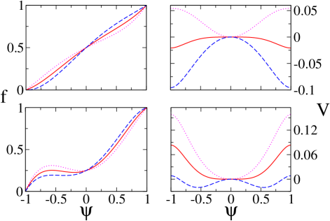
Figure 1: Flipping probability $f$ (left boxes) and its associated potential $V$ (right boxes) vs local field $\psi$. Curves correspond to coefficient values $a=-0.3$ (dotted), $a=0$ (solid), $a=0.3$ (dashed), for $b=-0.25$ (top) and $b=1.0$ (bottom). For both values of $b$, a single-well and double-well potentials are obtained for $a<0$ and $a>0$ respectively.

We performed numerical simulations on a $2$-dimensional square lattice with first-nearest neighbors (1st-NNs) interactions ($z=4$). We used flipping probabilities that are polynomial functions of the form of Eq. (4), for $b=-0.25$, $0.5$ and $3.0$, and various values of $a$ (see Fig. 1). Coefficients $c$ and $d$ were set in order to make $f$ an increasing function of $\psi$, and to arbitrarily fix the point $f(\psi=1)=1$. Starting from an ordered configuration of down spins (initial quenching), we flipped the spins of four neighboring sites at the center of the lattice and let the system evolve. We found that the average density of up spins $N$ and the survival probability $P$, for the three values of $b$, decay at the critical transition point $a_{GV}$ as $N\sim t^{\eta}$ and $P\sim t^{-\delta}$ (not shown), where $\eta\simeq 0$ and $\delta\simeq 0.95$ agree with the exponents $0$ and $1.0$ respectively, of the GV universality class Odor03 ; Dickman95 . Also, we found that the average density of interfaces has, at $a_{GV}$, a logarithmic decay with time ($\rho\simeq\pi/(2\ln t)$), as in the VM Krapivsky92-Frachebourg96 . Surprisely, only a GV transition was observed for all three values of $b$, in contradiction with Hammal05 .

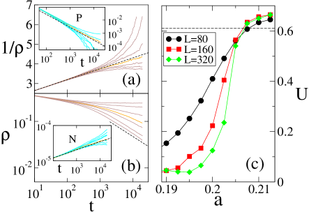
Figure 2: GV, DP and Ising transitions on a $2D$ square lattice of side $L=400$ with up to 3rd-NNs ($z=12$). (a) $1/\rho$ vs time on a log-linear scale, for $b=-0.25$ and values of $a$ around the GV critical point $a_{GV}\simeq-0.1105$. (b) $\rho$ vs time on a log-log scale for $b=0.5$ and values of $a$ around the DP critical point $a_{DP}\simeq 0.2127$. (c) Binder cumulant $U$ vs $a$ for $b=0.5$. Curves cross at $a_{I}\simeq 0.205$, where $U\simeq 0.56$, close to the universal value $0.6107$ of the $d=2$ Ising model (horizontal dashed line). Insets: (a) survival probability $P$ and (b) density of up spins $N$, on a $800^{2}$ lattice, starting from a quenched configuration. Curves are averages over $10^{5}$ realizations. Dashed straight lines have slopes $2/\pi$ and $-1$ in (a) and its inset respectively, whereas the slopes are $-0.45$ and $0.2295$ in (b).

However, our results are in agreement with that of Dornic et. al. Dornic01 where, by studying the dynamics of coarsening without surface tension (also with 1st-NNs interactions), they conjectured that all models with $Z_{2}$-symmetry and without bulk noise exhibit GV transitions. This apparent disagreement between theory (three transitions) and simulations (only GV transition) comes from the fact that Ising dynamics is observed when there is bulk noise, and this happens in our model when the interaction distance is equal or larger than $2$. Thus, a spin surrounded by $8$ parallel spins can still flip if at least one of the four 3-rd NNs is antiparallel. Indeed, simulations taking up to 2-nd NNs ($z=8$) also revealed GV only, but increasing the interactions up to 3-rd NNs ($z=12$), all GV, Ising and DP transitions were observed. This agrees with the work by Droz et al. Droz03 , in which they studied an absorbing Ising model in two dimensions, and found that extending the interaction range up to $z=12$ neighbors, the transition from disorder to order splits into a first Ising transition that breaks the symmetry, and then a DP transition to the unique absorbing state selected by the spontaneous symmetry breaking.

In Fig. 2 we plot the numerical results for $z=12$ neighbors. We see that for $b=-0.25$ (Fig.2(a)), the decay of $\rho$ and $P$ at $a_{GV}\simeq-0.1105$ correspond to that of a GV transition, whereas for $b=0.5$ (Fig. 2(b)), the transition to complete order happens at a value $a_{DP}\simeq 0.2127$ at which $\rho\sim t^{-\delta}$, $N\sim t^{\eta}$ and $P\sim t^{-\delta}$ (not shown), with $\delta\simeq 0.45$ and $\eta\simeq 0.2295$, i.e. DP critical exponents. In order to find the Ising transition, we calculated the Binder cumulants $U=1-m_{4}/3m_{2}^{2}$ (Fig. 2(c)), where $m_{4}$ and $m_{2}$ are the fourth and second moments of the magnetization, as a function of $a$. As we can see, at the critical point $a_{I}\simeq 0.205$, the curves of the Binder cumulants for different system sizes cross each other at the value $U\simeq 0.56$, similar to the universal value $0.6107$ of the $2D$ Ising model.

Conclusions. Summing up, we have derived from the microscopic dynamics, the Langevin equation for the magnetization field of general non-equilibrium spin systems with two symmetric absorbing states. This equation agrees with the one introduced in previous work, but now the dependence of the different terms on the flipping probability is explicitly stated. This methodology allows to predict the macroscopic behavior, such as critical properties and ordering dynamics, by simply knowing the derivatives of the transition probabilities. A large class of models in many different disciplines can be studied in this way. The generalization of this approach to models with an arbitrary number of symmetric absorbing states seems to be challenging.

We are very grateful to Maxi San Miguel and Miguel A. Muñoz for fruitful discussions. We acknowledge support from project FISICOS (FIS2007-60327) of MEC and FEDER, and NEST-Complexity project PATRES (043268).

References

- (1) H. Hinrichsen, Adv. Phys. 49, 815 (2000).
- (2) G. Ódor, Rev. Mod. Phys. 76, 663 (2004).
- (3) O. Al Hammal, H. Chaté, I. Dornic, and M. A. Muñoz, Phys. Rev. Lett. 94, 230601 (2005).
- (4) I. Dornic, H. Chaté, J. Chave, and H. Hinrichsen, Phys. Rev. Lett. 87, 045701 (2001).
- (5) M. Droz, A. L. Ferreira, and A. Lipowski, Phys. Rev. E 67, 056108 (2003).
- (6) P. Clifford and A. Sudbury, Biometrika, 60, 581 (1973).
- (7) G. J. Baxter, R. A. Blythe and A. J. MacKane, Math. Biosci. 209, 124 (2007).
-
(8)
P. L. Krapivsky, Phys. Rev. A 45,
1067 (1992);
L. Frachebourg and P. L. Krapivsky, Phys. Rev. E 53, R3009 (1996). - (9) C. Castellano, S. Fortunato and V. Loreto, arXiv:0710.3256 (2007).
- (10) D. M. Abrams and S. H. Strogatz, Nature 424, 900 (2003).
- (11) L. Dall’Asta and C. Castellano, Europhys. Lett. 77, 60005 (2007).
- (12) H.-U. Stark, C. J. Tessone, and F. Schweitzer, Phys. Rev. Lett. 101, 018701 (2008).
- (13) X. Castelló, V. M. Eguíluz and M. San Miguel, New Journal of Physics 8, 308 (2006).
- (14) A. Baronchelli, L. Dall’Asta, A. Barrat, and V. Loreto, Phys. Rev. E 73, R015102 (2006).
- (15) L. Dall’Asta and T. Galla, arXiv:0806.0817 (2008).
- (16) F. Schweitzer and L. Behera, arXiv:cond-mat/0307742 (2008).
- (17) A. J. Bray, Adv. Phys. 51, 481 (2002).
- (18) R. Dickman, and A. Yu. Tretyakov, Phys. Rev. E 52, 3218 (1995).