Dynamics of a FitzHugh-Nagumo system subjected to autocorrelated noise

Abstract

We analyze the dynamics of the FitzHugh-Nagumo (FHN) model in the presence of colored noise and a periodic signal. Two cases are considered: (i) the dynamics of the membrane potential is affected by the noise, (ii) the slow dynamics of the recovery variable is subject to noise. We investigate the role of the colored noise on the neuron dynamics by the mean response time (MRT) of the neuron. We find meaningful modifications of the resonant activation (RA) and noise enhanced stability (NES) phenomena due to the correlation time of the noise. For strongly correlated noise we observe suppression of NES effect and persistence of RA phenomenon, with an efficiency enhancement of the neuronal response. Finally we show that the self-correlation of the colored noise causes a reduction of the effective noise intensity, which appears as a rescaling of the fluctuations affecting the FHN system.

I Introduction

Physical and biological systems are continuously perturbed by random fluctuations produced by noise sources always present in open systems Complex . In physical and biological systems, noise can be responsible for several interesting and counterintuitive effects.  Resonant activation (RA) and noise enhanced stability (NES) are two noise activated phenomena that have been widely investigated in a dissipative optical lattice, spin systems, Josephson junctions, chemical and biological complex systems, and financial markets RA ; NES ; Nes-theory ; SR . Because of the stochastic resonance phenomenon, a weak electric stimulus can be enhanced up to the detection threshold of the neural system Wiesenfeld .
Recently the increasing interest in neuronal dynamics gave rise to many studies in this field. Two approaches, widely used to investigate the neuron response to an external stimulus, are the Hodgkin-Huxley model Hodgkin and its simplified version, the FitzHugh-Nagumo (FHN) model Bonhoeffer ; van_der_Pol ; FitzHugh ; Hale ; Rocsoreanu ; Nagumo ; Keener . A FHN system, in the presence of fluctuations, because of its intrinsic nonlinearity, can give rise to interesting noise induced phenomena: modification of detection threshold by manipulation of noisy parameters Pei , noise-induced activation and coherence resonance Pikovsky , stochastic resonance in the presence of colored noise with a $1/f^{\beta}$ spectrum ($0\leq\beta\leq 2$) Nozaki , optimization of the interspike time and dependence of neuron firing on subthreshold periodic signal and additive noise Longtin , resonant activation and noise enhanced stability Pankratova .
Despite the broad interest in FHN system, however, understanding the role of the fluctuations and their correlation in nerve cells still remain elusive. This is why it is of particular importance the investigation of the mean response time of a single neuron-like element as a function of the noise parameters in the presence of various external perturbations.
In this paper, by using a colored noise given by the archetypal Ornstein-Uhlenbeck process, with correlation time $\tau$, we study the role of the fluctuations on the FHN system. In particular we analyze the mean response time (MRT) as a function both of the noise intensity and the correlation time and we find that the RA and NES phenomena observed in the presence of white noise Pankratova show meaningful modifications when a colored noise source is used. The paper is organized as follows. In the first paragraph we shortly introduce the Hodgkin-Huxley (HH) system, the archetypal model to describe neuronal dynamics, and the FitzHugh-Nagumo (FHN) system, which is a simplified version of the HH model, discussing briefly the motivations for using, instead of the more realistic HH approach, the FHN model. In order to analyze the dynamics of a single neuron, we take into account a FHN system driven by a periodic signal and we analyze the deterministic dynamics. Afterwards we investigate the stochastic FHN system. In particular we consider the effects of the fluctuations by inserting in the deterministic FHN model a colored noise source. We analyze two different cases: the noise affects the dynamics of the membrane potential (case I), the recovery variable is subject to noise (case II). We introduce the mean response time (MRT) in order to calculate the response time of the neuron, that is the time that the membrane potential takes to reach a given threshold. Finally we show that the self-correlation of the colored noise causes a reduction of the effective noise intensity, that is a rescaling effect of the fluctuations affecting the FHN system. In the last section we draw the conclusions.

II Hodgkin-Huxley model

In the year 1952 Alan Lloyd Hodgkin and Andrew Huxley proposed a neuronal model to describe the dynamics of an action potential. This consists in a ”spike” of electrical discharge generated as response to an external stimulus and travelling along the membrane of a cell. The Hodgkin-Huxley (HH) model, which consists of four nonlinear ordinary differential equations, describes the electrical characteristics of excitable cells such as neurons and cardiac myocytes, explaining the ionic mechanisms responsible for the appearance and propagation of action potentials in the squid giant axon Hodgkin . The semipermeable cell membrane separates the interior of the cell from the extracellular liquid and acts as a capacitor. If an input current $I(t)$ is injected into the cell, it may add further charge on the capacitor, or leaks through the channels in the cell membrane. Because of active ion transport through the cell membrane, the ion concentration inside the cell is different from that in the extracellular liquid. The Nernst potential generated by the difference in ion concentration is represented by a battery. Therefore the Hodgkin-Huxley type model represents the biophysical characteristic of cell membranes.

The HH model consists of four equations. The first one, given by

$$C\frac{du}{dt}=-\sum_{k}I_{k}+I.$$ (1)

with

$$\sum_{k}I_{k}=g_{Na}m^{3}h(u-E_{Na})+g_{K}n^{4}(u-E_{K})+g_{L}(u-E_{L}).$$ (2)

provides the dynamics of the voltage u across the membrane and $I_{k}$ is the sum of the ionic currents which pass through the cell membrane. The conservation of electric charge on a piece of membrane implies that the applied current $I(t)$ may be split in a capacitive current $I_{c}=Cdu/dt$ which charges the capacitor $C$ and further components $I_{k}$ which pass through the ion channels: a sodium channel with index $Na$, a potassium channel with index $K$ and an unspecific leakage channel with resistance $R$. All channels may be characterized by their resistance or, equivalently, by their conductance. The leakage channel is described by a voltage-independent conductance $g_{L}=1/R$; the conductance of the other ion channels is voltage and time dependent. If all channels are open, they transmit currents with a maximum conductance $g_{Na}$ or $g_{K}$, respectively. The parameters $E_{Na}$, $E_{K}$, and $E_{L}$ are the reversal potentials. Reversal potentials and conductances are empirical parameters whose values, referred to a voltage scale where the resting potential is zero, were obtained by Hodgkin and Huxley Hodgkin . The three additional variables $m$, $n$, and $h$ describe the probabilities that the two channels are open. The combined action of $m$ and $h$ controls the $Na^{+}$ channels. The $K^{+}$ gates are controlled by $n$. The three variables $m$, $n$, and $h$ are called gating variables. They evolve according to the differential equations

$$\frac{dm}{dt} = \alpha_{m}(u)\thinspace(1\thinspace-\thinspace m)\thinspace-\thinspace\beta_{m}(u)\thinspace m$$ (3)

$$\frac{dn}{dt} = \alpha_{n}(u)\thinspace(1\thinspace-\thinspace n)\thinspace-\thinspace\beta_{n}(u)\thinspace n$$ (4)

$$\frac{dh}{dt} = \alpha_{h}(u)\thinspace(1\thinspace-\thinspace h)\thinspace-\thinspace\beta_{h}(u)\thinspace h.$$ (5)

The functions $\alpha_{m}$, $\alpha_{n}$, $\alpha_{h}$, $\beta_{m}$, $\beta_{n}$, $\beta_{h}$ are empirical functions of $u$ that have been adjusted by Hodgkin and Huxley to fit the data of the giant axon of the squid. The four equations (1),(3)-(5) define the Hodgkin-Huxley model.

III FitzHugh-Nagumo model

The FitzHugh-Nagumo (FHN) model is a simpler version of the Hodgkin-Huxley model. In particular the FHN model takes into account the excitable variable, that is the membrane potential, which exhibits a fast dynamics, and the recovery variable, characterized by a slow dynamics and responsible for the refractory behaviour of the neuron. The reduction from four variables (HH model) to two variables (FHN model) allows to focalize the analysis on the properties of excitation and propagation, neglecting the specific electrochemical properties of sodium and potassium ion flow. Thus the neuron dynamics can be described in terms of a voltage-like variable and a recovery variable. The former, governed by a cubic nonlinearity, provides a regenerative self-excitation by a positive feedback, the latter, subject to a linear dynamics, is responsible for a slower negative feedback.

The archetypal form for the FHN model is given by the following two equations

$$\dot{V}\thinspace=\thinspace f(V)\thinspace-\thinspace W\thinspace+\thinspace I$$ (6)

$$\dot{W}\thinspace=\thinspace a\thinspace(b\thinspace V\thinspace-\thinspace c\thinspace W)\thinspace+\thinspace d$$ (7)

where $f(V)$ is a polynomial of third degree, and $a$, $b$, $c$, $d$ are parameters with constant values.
Actually the Hodgkin-Huxley model is closer to the real behaviour of neuronal dynamics. However, only projections of its four-dimensional phase trajectories can be observed. On the other side, by using the FitzHugh-Nagumo model, the solution for the time behaviour of the neuronal response can be represented in a two-dimensional space. This permits to give a geometrical explanation of important biological phenomena connected with neuronal excitability and spike-generating mechanism. Eqs.(6),(7) provide the deterministic dynamics for a FHN neuron. In fact, in the presence of an external stimulus, with enough strong amplitude, the membrane voltage (fast variable) increases rapidly, crossing a threshold. This event (voltage spiking) represents the neuron firing, that is the nerve response due to the external stimulus. After spike generation the voltage goes rapidly under threshold and a refractory time occurs so that during this time no further firing is possible. This behaviour is represented in Fig. 1 where a $(V,W)$ trajectory and the two nullclines

$$W=\thinspace f(V)+\thinspace I$$ (8)

$$W=\thinspace\frac{b}{c}\thinspace V+\thinspace\frac{d}{ac}$$ (9)

are shown for $f(V)=V-\frac{V^{3}}{3}$, $\frac{b}{c}=1.25$, $\frac{d}{ac}=0.875$, $I=-0.001$.

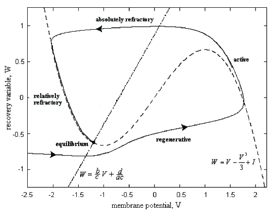
Figure 1: Phase diagram for FitzHugh-Nagumo model (modified from FitzHugh 1961 FitzHugh ). The (V,W) trajectory (solid line) after a spike event is in a refractory state, before reaching the equilibrium state which corresponds to the point where the two nullclines (dash line for $\dot{V}=0$ and dash-dot line for $\dot{W}=0$) intersect. Here we set $b/c=1.25$, $d/(ac)=0.875$, $I=-0.001$.

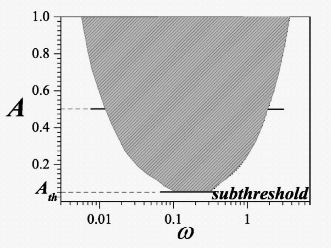
Figure 2: Parameter plane ($\omega$,$A$) for $\phi_{0}=0$. The grey zone corresponds to values of $\omega$ and $A$ for which deterministic firing occurs. The values of the parameters are $I=1.1$, $\epsilon=0.05$, $\varphi_{0}=0$. The initial state is $(x_{0},y_{0})$ (courtesy of Pankratova et al. Pankratova ).

IV FHN model with periodical driving signal

In the presence of a driving signal the FHN model becomes

$$\dot{x} = x-\frac{x^{3}}{3}-y+Asin(\omega\thinspace t+\varphi_{0})$$ (10)

$$\dot{y} = \epsilon(x+I),$$ (11)

where $\epsilon$ is a fixed small parameter which characterizes the recovery process, and $A$, $\omega$ are respectively amplitude and frequency of the external forcing.

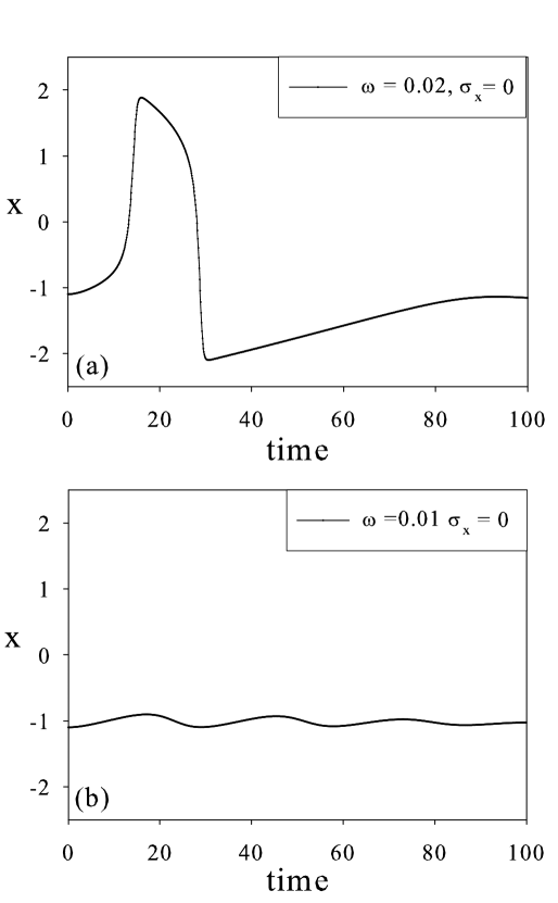
Figure 3: (a) The membrane potential $x$ exhibits a spike for $A=0.5$ and $\omega=0.02$ (deterministic firing region). (b) For $A=0.5$, $\omega=0.01$ no spike appears (deterministic no-firing region): the values of the parameters don’t allow the system to fire. Parameter values and initial conditions are the same of Fig. 2.

In the absence of an external driving force there is only one stationary state given by

$$x_{0} = -I$$ (12)

$$y_{0} = -I+I^{3}/3.$$ (13)

The first variable, $x$, represents the membrane potential which is characterized by a fast dynamics: after $x$ crosses the threshold value ($x=0$), rapidly it takes on values below the threshold and a period occurs during which no firing is possible. This condition is connected with the dynamics of the second variable, $y$, characterized by a slow dynamics. Depending on the value of $I$ the stationary point is unstable with stable periodic solution ($|I|<1$) or stable with all the trajectories converging on it (attractor) ($|I|>1$) Pankratova . Here we set $I=1.1$ and we take ($x_{0},y_{0}$) as initial state for the evolution of the FHN system. In this condition a time evolution occurs if the system is driven out of equilibrium. First, we consider the system in deterministic dynamical regime, that is, when firing events occur in the absence of noise (deterministic firing region). This regime takes place when values of amplitude and frequency are chosen inside the gray zone of the parameter plane (see Fig. 2) and corresponds to the situation shown in Fig. 3 (a)). Otherwise, when the neuron shows no excitability in the absence of noise, the system is in the deterministic no-firing region (see Fig. 3 (b)). This condition occurs when the values of $A$ and $\omega$ are chosen out of the gray zone of Fig. 2.

V The stochastic FHN model

Physical and biological systems are affected by the presence of continuous random perturbations, due to fluctuations of environmental parameters such as temperature and natural resources, which contribute to modify the system dynamics Complex .

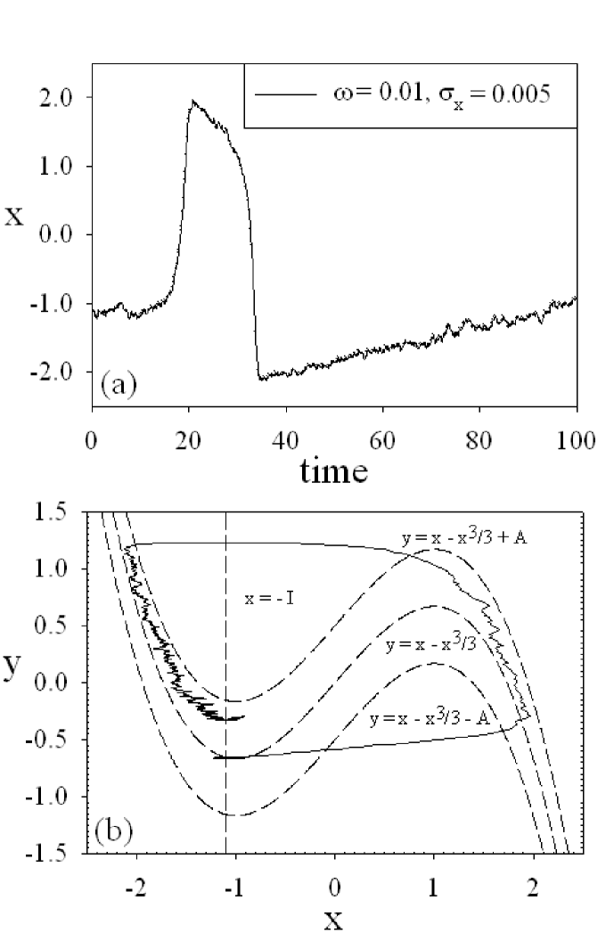
Figure 4: (a) and (b) Stochastic dynamics and corresponding trajectory in the space ($x,y$) for $A=0.5$, $\omega=0.01$: because of the cooperative action of external signal and fluctuations a stochastic evolution appears that allows the system to fire out of the deterministic firing region. Parameter values and initial conditions are the same of Fig. 2.

These fluctuations can be modeled by inserting a noise term in the deterministic equations. In this work we consider the neuron as an open system whose dynamics is affected by the presence both of periodic and random variations of environmental parameters. Therefore we modify the deterministic FHN model by adding a colored noise term. In particular we consider two different cases: i) the membrane potential is subject to a noisy dynamics (Case I); ii) the refractory variable, which describes the recovery properties of the neuron, is exposed to fluctuations (Case II). From Eqs. (10),(11) we get

$$Case\enspace I$$

$$\dot{x} = x-\frac{x^{3}}{3}-y+Asin(\omega\thinspace t+\varphi_{0})+\zeta_{x}$$

$$\dot{y} = \epsilon(x+I),$$ (14)

$$Case\enspace II$$

$$\dot{x} = x-\frac{x^{3}}{3}-y+Asin(\omega\thinspace t+\varphi_{0})$$

$$\dot{y} = \epsilon(x+I)+\zeta_{y},$$ (15)

where $\zeta_{i}(t)$ ($i=x,y$) are self-correlated noises described by Ornstein-Uhlenbeck processes Gardiner

$$\frac{d\zeta_{i}}{dt}=-\frac{1}{\tau}\zeta_{i}(t)+\frac{1}{\tau}\xi_{i}(t).$$ (16)

Here $\tau$ is the correlation time of the noise, and $\xi_{i}(t)$ are statistically independent Gaussian white noises with zero mean and correlation function

$$<\xi_{i}(t)\xi_{j}(t^{\prime})>=\sqrt{\sigma_{i}}\thinspace\sqrt{\sigma_{j}}\thinspace\delta_{ij}\thinspace\delta(t-t^{\prime})\quad(i,j=x,y)$$ (17)

The correlation function of the process given by Eq. (16) is

$$\langle\zeta_{i}(t)\zeta_{j}(t^{\prime})\rangle=\frac{\sqrt{\sigma_{i}}\thinspace\sqrt{\sigma_{j}}\thinspace}{2\tau}e^{-|t-t^{\prime}|/\tau}\delta_{ij}$$ (18)

with

$$lim_{\tau\rightarrow 0}\langle\zeta_{i}(t)\zeta_{j}(t^{\prime})\rangle=\sqrt{\sigma_{i}}\thinspace\sqrt{\sigma_{j}}\thinspace\delta(t-t^{\prime})\delta_{ij}.$$ (19)

In a previous work the system response has been studied, under the influence of a periodic driving signal, as a function of the white noise intensity Pankratova . The authors showed the occurrence of resonant activation (RA) and noise enhanced stability (NES). In particular the presence of a noise source is responsible for modifications in the resonant activation phenomenon and causes noise enhanced stability to appear in the minimum. NES effect and modifications in RA, observed in the deterministic firing region (grey zone in Fig.2), are connected with the appearance of neuron excitability even if the parameters $A$ and $\omega$ take values out of this region. In fact, by setting $A=0.5$, $\omega=0.01$ with $\tau\rightarrow 0$ (white noise) and $\sigma_{x}=0.005$ (Case I), the FHN system can fire also for parameter values chosen in the deterministic no-firing region (see Fig. 4). Because of the cooperative action of periodic force and noise, a stochastic evolution appears that allows the system to fire out of the deterministic firing region. However, a self-correlated noise represents a model more suitable to represent the random fluctuations in real systems, where the noise spectrum is characterized by the presence of a cut-off. Therefore, in this paper we study the system response, in the presence of a periodic driving signal, by using the colored Gaussian noise given by Eq. (16) Valenti .

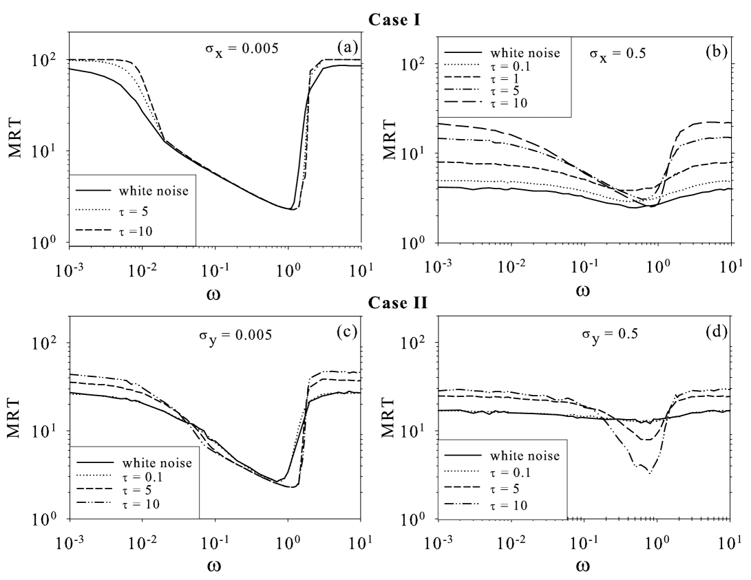
Figure 5: (a) and (c): For low noise intensities a slight displacement of the RA minimum is observed as the correlation time $\tau$ increases (weak suppression of the noise effects). (b) and (d): For higher noise intensities the minimum of RA is strongly affected by the value of $\tau$. Both in cases I and II the RA minimum almost disappears for white noise, while it is more pronounced for high values of $\tau$ (strong suppression of the noise effects). Parameter values and initial conditions are the same of Fig. 2.

VI Results

In order to investigate the dynamics of FHN system we analyze the behaviour of the mean response time (MRT) of the neuron when periodical stimulus and colored noise are present. Therefore we don’t consider the periodicity of the signal. MRT is defined as $<T>\thinspace=\thinspace 1/N\sum_{i=1}^{N}T_{i}$. Here $T_{i}$ is the first response time (that is, the time for which the first spike occurs) of the $i^{th}$ realization and $N$ is the total number of realizations. In order to calculate MRT we solve Eqs. (14, 15) by performing numerical simulations, with $N=5000$ for case I (the membrane potential is subject to fluctuations) and $N=15000$ for case II (the refractory variable is noisy). For all realizations the amplitude value of the external driving force and the initial conditions are $A=0.5$ and $(x_{0},y_{0})$, respectively. We consider a spike occurred when $x$ gets over the threshold value $x_{thr}=0$. We observe Resonant Activation (RA) and Noise Enhanced Stability (NES) phenomena both in cases I and II.

VI.1 Resonant Activation

In Fig. 5 we report MRT as a function of $\omega$ for different values both of noise intensities $\sigma_{x}$, $\sigma_{y}$ and correlation time $\tau$. The value of the RA minimum is affected by the noise intensity. For a low level of noise (see Fig. 5(a), (c)) this minimum is well pronounced, without any significative modifications occur as the correlation time $\tau$ increases. We name this weak suppression of the noise effects. However, at higher noise intensities, $\sigma_{x}=0.5$ and $\sigma_{y}=0.5$, (see Fig. 5(b), (d)), the correlation time becomes more relevant, so that the value of the RA minimum depends strongly on $\tau$. In particular, as $\tau$ increases, the minimum is closer to the values of the deterministic regime. In this case we say that a strong suppression of the noise effects occurs. In particular, in case I we find a nonmonotonic behaviour of MRT as a function of $\tau$ in the frequency range $0.1<\omega<1.5$.

VI.2 Noise Enhanced Stability

By comparing panels (a) and (b) in Fig. 5 for $\tau=0$ (white noise) and $\tau=5,\enspace 10$, we observe, in case I (membrane potential is subject to fluctuations), an enhancement of the MRT due to the noise, that is, the depth of RA minimum is reduced as the noise intensity increases. This enhancement of MRT indicates that higher levels of noise cause a ”response delay” and reduce the neural efficiency. Extensively we consider this behaviour as NES effect. A comparison between panels (c) and (d) of Fig. 5 shows that the same phenomenon is present also in case II (refractory variable is noisy).

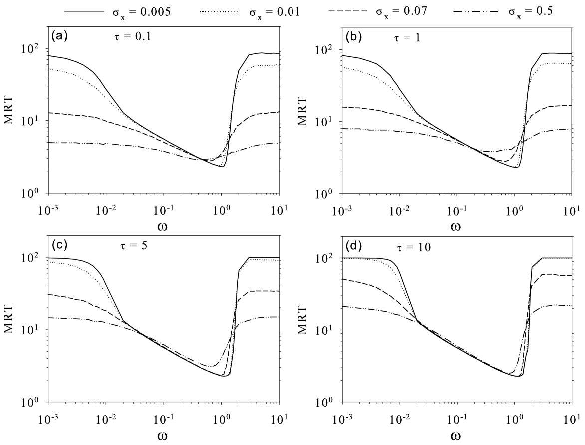
Figure 6: Case I. For weakly correlated noise ($\tau=0.1$) MRT shows a nonmonotonic behaviour as a function of the noise intensity (see panel (a)). For higher values of the correlation time ($\tau=1$) this effect is reduced (see panel (b)). In the presence of strongly correlation ($\tau=5$, $\tau=10$) this phenomenon disappears and the depth of RA minimum becomes almost independent on the noise intensity (suppression of the noise effect)(see panels (c), (d)). Parameter values and initial conditions are the same of Fig. 2.

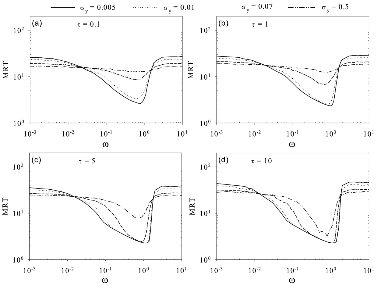
Figure 7: Case II. For weakly correlated noise ($\tau=0.1$) a monotonic behaviour of MRT as a function of the noise intensity appears (see panel (a)). As the correlation time increases ($\tau=1$) this phenomenon is attenuated (see panel (b)). Finally, for strongly correlation ($\tau=5$, $\tau=10$) the depth of RA minimum is almost independent on the noise intensity (suppression of the noise effect). Parameter values and initial conditions are the same of Fig. 2.

In view of a better understanding of this effect, we analyze further the behavior of the mean response time. In particular, we calculate the MRT as a function of the noise intensity for different values of the correlation time. The results are shown in Figs. 6, 7. We note that a weakly correlated noise source affects significatively the efficiency of the neuronal response. In particular, for $\tau=0.1,1$ we observe that, both in cases I and II, the depth of RA minimum decreases for high levels of noise, which is an enhancement of MRT due to the noise (NES effect) (see Figs. 6a,b and 7a,b). Conversely, in the presence of strongly correlated noise, no lack of efficiency is observed around the RA minimum, which maintains its depth almost unchanged as noise intensity increases (see Figs. 6c,d and 7d). This behavior can be evidenced by taking into account the values of MRT in the RA minimum. From Figs. 6 and 7 we note that the position of the minimum, for the lowest values of the correlation time and the noise intensity ($\tau=0.1$ and $\sigma=0.005$), is given by $\omega\simeq 1$ for case I and $\omega\simeq 0.7$ for case II. Therefore we calculate MRT as a function of the noise intensity for different values of $\tau$, setting $\omega=1$ in case I and $\omega=0.7$ in case II. The results are reported in Fig. 8.

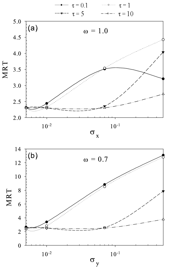
Figure 8: (a) Case I. Nonmonotonic behaviour (with a maximum) of MRT as a function of the noise intensity $\sigma_{x}$, for $\omega=1.0$: in the presence of colored noise this effect disappears as correlation time increases. (b) Case II. Monotonic increase of MRT as a function of the noise intensity $\sigma_{y}$, for $\omega=0.7$: this behaviour is suppressed for strongly correlated noise. Parameter values and initial conditions are the same of Fig. 2.

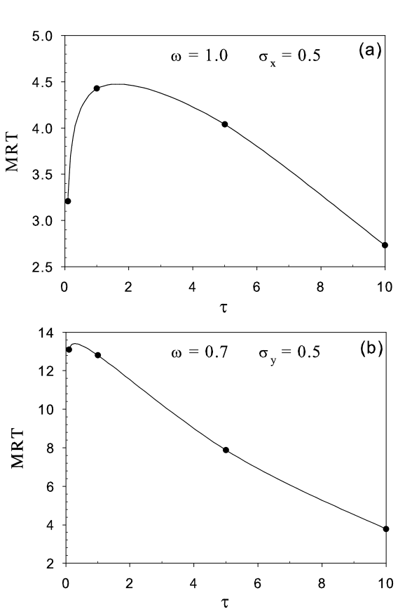
Figure 9: (a) Case I. Nonmonotonic behaviour of the MRT as a function of the correlation time $\tau$, for $\omega=1.0$ and $\sigma_{x}=0.5$. (b) Case II. Decrease of the MRT as a function of the correlation time $\tau$, for $\omega=0.7$ and $\sigma_{y}=0.5$. Parameter values and initial conditions are the same of Fig. 2.

From the inspection of the figure we note that, in both cases, the strong dependence of the MRT on the noise intensity is suppressed as correlation time increases: the effect of the noise in the RA minimum (region of highest efficiency) appears to be smaller as $\tau$ increases. More precisely we note that, in case I, MRT shows in the minimum a nonmonotonic behavior as a function of $\sigma_{x}$: starting from $\sigma_{x}=0.005$ for intermediate levels of noise intensity an increase of MRT appears. For higher noise intensities a decrease of MRT is observed (see Fig. 8a). On the other side, for case II, a monotonic increase of MRT is observed as a function of the noise intensity $\sigma_{y}$. However, in both cases, for high values of the correlation time, MRT tends to be constant as the noise intensity increases, in the range of the noise intensity values investigated. The modifications induced by the noise in the mean response time are strongly reduced and they almost disappears for $\tau=10$ (suppression of the noise effects). Finally we note, in case I, a nonmonotonic behaviour of MRT as a function of the correlation time $\tau$. This behaviour appears for noise intensity values greater than $\sigma_{x}=0.07$, corresponding to the maximum of the curve for $\tau=0.1$. In Fig. 9 we report MRT vs $\tau$ both for case I and II with $\sigma=0.5$.

VI.3 Colored noise: rescaling effect

Let’s consider two colored Gaussian noise sources, $S1$ and $S2$, with the same intensity $\sigma$, characterized by the correlation times $\tau_{1}$ and $\tau_{2}$ respectively, with $\tau_{1}<\tau_{2}$. The behaviour shown in Fig. 8 indicates that the presence of a self-correlation causes a reduction of the noise ”efficacy”. This suggests that, for frequency values around the RA minimum, the noise effect on a FHN system is more intensive when one uses $S1$, that is the noise source characterized by the smaller correlation time. Remembering that the white noise is obtained by the colored noise in the limit $\tau\rightarrow 0$ (see Eq. (19)), one expects that, for frequency values around the RA minimum, a white noise source with intensity $\sigma$ influences the neural dynamics more than any correlated noise source with the same intensity $\sigma$.

From Eq. (19) we note that for $|t-t^{\prime}|<\tau$ we can approximate $e^{-|t-t^{\prime}|/\tau}\sim 1$. So that from Eq. (18) we get

$$\langle\zeta_{i}(t)\zeta_{j}(t^{\prime})\rangle\approx\frac{\sqrt{\sigma_{i}}\thinspace\sqrt{\sigma_{j}}\thinspace}{2\tau}\delta_{ij}.$$ (20)

This result could be interpreted as a rescaling effect: the correlation time seems to reduce the noise intensity of the colored noise by a factor equal to $2\tau$. This suggests that, in the RA minimum, the effect of a colored noise source with intensity $\sigma_{colored}$ and correlation time $\tau$ should be, for $|t-t^{\prime}|/\tau\sim 0$, the same obtained by using a white noise source with intensity given by

$$\sigma_{white}=\frac{\sigma_{colored}}{2\tau}.$$ (21)

Therefore we define the ”effective” intensity of a colored noise according to Eq. (21), when MRT is of the same order of magnitude of $\tau$ or less. In order to verify this rescaling effect we consider again the curve of Fig. 5d obtained for $\sigma_{y}=0.5$ and $\tau=5$ and we obtain the corresponding ”effective” noise intensity $\sigma_{white}=(\sigma_{colored})/2\tau=0.05$. Afterwards, by using this value we calculate the MRT as a function of $\omega$. The results have been reported in Fig. 10.

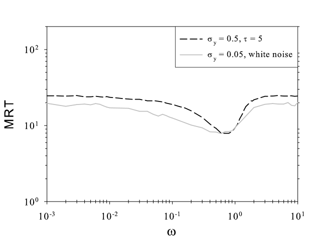
Figure 10: Case II. The correlation time causes a rescaling effect according to $\sigma_{white}=\sigma_{colored}/2\tau$. Around the minimum the curve obtained for $\sigma_{colored}=0.5$ and correlation time $\tau=5$ (black dash line) overlaps that obtained by using a white noise source with intensity $\sigma_{white}=\sigma_{colored}/2\tau=0.05$ (gray solid line). Parameter values and initial conditions are the same of Fig. 2.

In the figure we note that around the RA minimum, that is for $MRT\sim\tau$ and $e^{-|t-t^{\prime}|/\tau}\sim 1$, the influence of the colored noise in the FHN dynamics depends on the ”effective” noise intensity $\sigma_{white}=0.05$. This means that, in the presence of colored noise and for suitable values of the correlation time $\tau$, the actual noise intensity perceived by the FHN system is reduced by the rescaling factor $1/(2\tau)$. We recall that the white noise is a theoretical assumption to describe noise whose band width is very large. In fact, in real systems the fluctuations are connected with colored noise sources. Therefore, in order to evaluate the response of a real neuron, one has to consider self-correlated noise sources: the rescaling phenomenon, as we show in this paper, reduces the effect of the noise on the FHN dynamics, modifying in a significative way the neuronal dynamics.

VII Conclusions

After a brief discussion on the  Hodgkin-Huxley (HH) model, we introduce the FitzHugh-Nagumo (FHN) model. Although it is a simplified version of the former, the latter permits to separate the mathematical characteristics of excitation and propagation from the electrochemical peculiarities of sodium and potassium ion flows. Even if the HH model better describes the real dynamics of the neuronal response, it allows only to observe two-dimensional projections of its four-dimensional phase trajectories. Because of this, the FHN model is often preferred, providing the whole solution directly in a two-dimensional phase space. This characteristic permits to envisage a geometrical interpretation of important biological phenomena that depend on the spike-generating mechanism which causes the neuronal response to external stimuli. Therefore, in this paper we analyzed the response of a neuron in the presence both of a driving periodical force with frequency $\omega$ and an additive Gaussian colored noise, by the FHN neuronal model. In our analysis we considered two cases: I) the noise source affects the membrane potential, II) the noise source influences the recovery variable. In these conditions we analyzed the mean response time (MRT) as a function both of the noise intensity and the correlation time. We found that RA and NES phenomena undergo meaningful modifications due to the presence of different values of the correlation time $\tau$. For strongly correlated noise we observed suppression of NES and persistence of RA (efficiency enhancement of neuronal response) as correlation time $\tau$ increases. This indicates that the RA minimum corresponding to a certain value of $\omega$ is preserved when the noise source is characterized by large values of the correlation time. Conversely the enhancement of the MRT, which indicates a significant role of the noise, tends to vanish. The reduction of the noise effects in the presence of strongly correlated noise indicates a rescaling effect of the noise self-correlation. We investigated this aspect for a colored noise source whose intensity and correlation time are given by $\sigma$ and $\tau$ respectively. We found that, for $MRT\sim\tau$, an ”effective” noise intensity exists. This implies that the effect of the self-correlated noise can be reproduced, through a rescaling procedure, by using a white noise source whose amplitude is given by $\sigma_{white}=(\sigma_{colored})/2\tau$.

VIII Acknowledgments

Authors acknowledge the support by MUR. This work makes use of results produced by the PI2S2 Project managed by the Consorzio COMETA, a project co-funded by the Italian Ministry of University and Research (MIUR) within the Piano Operativo Nazionale Ricerca Scientifica, Sviluppo Tecnologico, Alta Formazione (PON 2000-2006). More information is available at http://www.pi2s2.it and http://www.consorzio-cometa.it.

References

- (1) See the special section on ”Complex Systems”, Science 284, (1999) 79-107; O. N. Bjornstad and B. T. Grenfell, Science 293, (2001) 638-643; S. Ciuchi, F. de Pasquale and B. Spagnolo, Phys. Rev. E 53, (1996) 706-716; M. Scheffer, S. R. Carpenter, J. A. Foley, C. Folke, B. Walker, Nature 413, (2001) 591-596; B. Spagnolo, D. Valenti, A. Fiasconaro, Math. Biosc. and Engineering 1, (2004) 185-211.
- (2) C. R. Doering and J. C. Gadoua, Phys. Rev. Lett. 69, (1992) 2318-2321; R. N. Mantegna and B. Spagnolo, Phys. Rev. Lett. 84, (2000) 3025-3028; P. Majee, G. Goswami, B. Chandra Bag, Chem. Phys. Lett. 416, (2005) 256-260; R. Gommers, P. Douglas, S. Bergamini, M. Goonasekera, P. H. Jones, and F. Renzoni, Phys. Rev. Lett. 94, (2005) 143001(1-4).
- (3) R. N. Mantegna, B. Spagnolo, Phys. Rev. Lett. 76, (1996) 563-566; R. Wackerbauer, Phys. Rev. E 59, 2872 (1999); A. Mielke, Phys. Rev. Lett. 84, (2000) 818-821; B. Spagnolo, A. A. Dubkov, and N. V. Agudov, Acta Phys. Pol. 35, (2004) 1419-1436; G. Bonanno, D. Valenti and B. Spagnolo, Phys. Rev E 75, (2007) 016106(1-8).
- (4) N. V. Agudov, B. Spagnolo, Phys. Rev. E 64, (2001) 035102(1-4); A. A. Dubkov, N. V. Agudov and B. Spagnolo, Phys. Rev. E 69, (2004) 061103(1-7).
- (5) E. Lanzara, R. N. Mantegna, B. Spagnolo and R. Zangara, Am. J. Phys. 65, (1997) 341-349; L. Gammaitoni, P. Hänggi, P. Jung, F. Marchesoni, Rev. Mod. Phys. 70, (1998) 223-288; Y. Kashimori, H. Funakubo, and T. Kambara, Biophys. J. 75, (1998) 1700-1711; D. Valenti, A. Fiasconaro, B. Spagnolo, Phys. A 331, (2004) 477 486; B. Kosko and S. Mitaim, Phys. Rev. E 70, (2004) 031911 (1-10); A. Caruso, M. E. Gargano, D. Valenti, A. Fiasconaro, B. Spagnolo, Fluc. Noise Lett. 5, (2005) L349-L355.
- (6) K. Wiesenfeld, F. Moss Nature 373, (1995) 33-36; F. Chapeau-Blondeau, X. Godivier, and N. Chambet Phys. Rev. E 53, (1996) 1273-1275 ; Special Issue: Advances in neural networks research IJCNN’03, B. Kosko, S. Mitaim, Neural Networks 16, (2003) 755-761.
- (7) A. L. Hodgkin and A. F. Huxley, J. Physiol. 117, (1952) 500-544; E.V. Pankratova, A.V. Polovinkin, E. Mosekilde, Eur. Phys. J. B 45, (2005) 391-397; V.N. Belykh and E.V. Pankratova, Dynamics and synchronization of noise perturbed ensembles of periodically activated neuron cells, Int. J. Bifurcation and Chaos 18, (2008) in press.
- (8) K. F. Bonhoeffer, J. Gen. Physiol. 32, (1948) 69-91; K. F. Bonhoeffer, Naturwissenschaften 40, (1953) 301-311.
- (9) B. van der Pol and J. van der Mark, Arch. Néerl. Physiol. 14, (1929) 418-443 .
- (10) R. FitzHugh, Bull. Math. Biophysics 17, (1955) 257-278; R. FitzHugh, J. Gen. Physiol. 43, (1960) 867-896; R. FitzHugh, Biophys. J. 1, (1961) 445-466.
- (11) J. H. Hale, H. Kocak, Dynamics and Bifurcations (Springer-Verlag, New York 1991).
- (12) C. Rocsoreanu, A. Georgescu, N. Giurgiteanu, The FitzHugh-Nagumo Model: Bifurcation and Dynamics (Kluwer Academic Publishers, Boston 2000).
- (13) J. Nagumo, S. Arimoto, and S. Yoshizawa, Proc. IRE 50, (1964) 2061-2070.
- (14) J. Keener, J. Sneyd, Mathematical Physiology (Springer-Verlag, New York 1998).
- (15) X. Pei, K. Bachmann and F. Moss, Phys. Lett. A 206, (1995) 61-65.
- (16) A. S. Pikovsky, and J. Kurths, Phys. Rev. Lett. 78, (1997) 775-778.
- (17) D. Nozaki, Y. Yamamoto, Phys. Lett. A 243, (1998) 281-287.
- (18) A. Longtin, D. R. Chialvo, Phys. Rev. Lett. 81, (1998) 4012-4015.
- (19) E. V. Pankratova, A. V. Polovinkin, B. Spagnolo, Phys. Lett. A 344, (2005) 43-50.
- (20) C. W. Gardiner, Handbook of Stochastic Methods for Physics, Chemistry and the Natural Sciences, (Springer, Berlin 1993).
- (21) D. Valenti, A. Fiasconaro and B. Spagnolo, Mod. Prob. Stat. Phys. 2, (2003) 91-100; D. Valenti, A. Fiasconaro and B. Spagnolo, Fluc. Noise Lett. 5, (2005) L337-L342; D. Valenti, L. Schimansky-Geier, X. Sailer, B. Spagnolo, M. Iacomi, A. Phys. Pol. B 38, (2007) 1961-1972.