Determination of the Strong Coupling $\alpha_{\mathrm{S}}$ from hadronic Event Shapes with ${\cal O}(\alpha_{\mathrm{S}}^{3})$ and resummed QCD predictions using JADE Data

Abstract

Event Shape Data from $\mathrm{e^{+}e^{-}}$ annihilation into hadrons collected by the JADE experiment at centre-of-mass energies between 14 GeV and 44 GeV are used to determine the strong coupling $\alpha_{\mathrm{S}}$. QCD predictions complete to next-to-next-to-leading order (NNLO), alternatively combined with resummed next-to-leading-log-approximation (NNLO+NLLA) calculations, are used. The combined value from six different event shape observables at the six JADE centre-of-mass energies using the NNLO calculations is

$$\alpha_{\mathrm{S}}(m_{\mathrm{Z^{0}}})=0.1210\pm 0.0007\mathrm{(stat.)}\pm 0.0021\mathrm{(exp.)}\pm 0.0044\mathrm{(had.)}\pm 0.0036\mathrm{(theo.)}$$

and with the NNLO+NLLA calculations the combined value is

$$\alpha_{\mathrm{S}}(m_{\mathrm{Z^{0}}})=0.1172\pm 0.0006\mathrm{(stat.)}\pm 0.0020\mathrm{(exp.)}\pm 0.0035\mathrm{(had.)}\pm 0.0030\mathrm{(theo.)}\;\;.$$

The stability of the NNLO and NNLO+NLLA results with respect to missing higher order contributions, studied by variations of the renormalisation scale, is improved compared to previous results obtained with NLO+NLLA or with NLO predictions only. The observed energy dependence of $\alpha_{\mathrm{S}}$ agrees with the QCD prediction of asymptotic freedom and excludes absence of running with 99% confidence level.

1 Introduction

Analyses of events originating from $\mathrm{e^{+}e^{-}}$ annihilation into hadrons allow studies biebel01a ; dasgupta03 ; dissertori03 ; kluth06 of Quantum Chromodynamics (QCD), the theory of the strong interaction fritzsch73 ; gross73a ; gross73b ; politzer73 . Comparison of observables like jet production rates or event shapes with theoretical predictions provides access to the determination of the strong coupling $\alpha_{\mathrm{S}}$. Recently significant progress in the theoretical calculations of event shape observables has been made and next-to-next-to-leading order (NNLO) predictions are now available gehrmannderidder07b as well as matching with resummed calculations in the next-to-leading-log-approximation (NLLA) gehrmann08 . As a first application, measurements of $\alpha_{\mathrm{S}}$ at centre-of-mass-system (cms) energies between $\sqrt{s}=91$ GeV and $\sqrt{s}=206$ GeV were presented dissertori07 . The same theoretical predictions are used in this paper to determine the strong coupling $\alpha_{\mathrm{S}}$ from JADE data recorded at lower cms energies. As in dissertori07 and the previous standard LEP and JADE analyses kluth06 we use Monte Carlo simulations to treat hadronisation effects. In davison08 data for thrust at cms energies $14\leq\sqrt{s}\leq 207$ GeV are analysed with combined NNLO+NLLA calculations and an analytic model for non-perturbative physics.

The JADE experiment operated at the PETRA $\mathrm{e^{+}e^{-}}$ collider at DESY, Hamburg, Germany. The data taken in the years from 1979 to 1986 cover cms energies between 12 and 46.4 GeV.

2 The JADE Detector

A detailed description of the JADE detector can be found in naroska87 . For this analysis, tracks from charged particles and energy deposits in the electromagnetic calorimeter are used. The main tracking device, a large volume jet chamber was located in a 0.48 T solenoidal magnetic field. The electromagnetic calorimeter consisted of 2520 lead glass blocks in the barrel and 192 lead glass blocks in both endcaps with radiation length varying between 9.6 in the endcaps and up to 15.7 in the barrel.

3 Data and Monte Carlo Samples

The Data and Monte Carlos samples utilised in this analysis are identical to those used in a previous determination of $\alpha_{\mathrm{S}}$ jader4 . The data correspond to a total integrated luminosity of 195/pb taken at average cms energies between 14.0 GeV and 43.8 GeV. The breakdown of the data samples, including the average cms energies, the energy ranges, data taking periods, integrated luminosities and the overall numbers of selected hadronic events are summarised in table 1.

Table 1: The average centre-of-mass energy $\sqrt{s}$, the energy range, data taking period, collected integrated luminosity $L$ together with the number of selected data events.

$\sqrt{s}$	energy	year	$L$	selected
GeV	range in GeV		(1/pb)	events
14.0	13.0–15.0	1981	1.46	1783
22.0	21.0–23.0	1981	2.41	1403
34.6	33.8–36.0	1981–1982	61.7	14313
35.0	34.0–36.0	1986	92.3	20876
38.3	37.3–39.3	1985	8.28	1585
43.8	43.4–46.4	1984–1985	28.8	4374

Monte Carlo events are generated in large numbers to correct the data for experimental acceptance, resolution effects and background. Events are simulated using PYTHIA 5.7 jetset3 , and for systematic studies with HERWIG 5.9 herwig . Subsequently the generated events are processed through a full simulation of the JADE detector and are reconstructed in the same way and with the same program chain as the data. For comparison with the corrected data and for the correction of hadronisation effects large samples of Monte Carlo events have been produced using PYTHIA 6.158, HERWIG 6.2 and ARIADNE 4.11 ariadne3 . We use the model parameters as determined at $\sqrt{s}$=91 GeV by the OPAL experiment at the LEP $\mathrm{e^{+}e^{-}}$ collider OPALPR141 ; OPALPR379 .

4 Experimental Procedure

4.1 Event Selection

The selection of identified and well measured hadronic event candidates follows the procedure outlined in jader4 . Events with a large momentum imbalance due to photons emitted in the initial state are rejected. The event selection is based on minimal requirements for charged particle multiplicity, visible energy and longitudinal momentum imbalance. The dominating backgrounds from hadronic $\tau$ decays and two-photon interactions with hadronic final states are supressed to negligble levels.

4.2 Event Shape Distributions

The properties of hadronic events can be described by event shape observables. Event shape observables used for this analysis are thrust ($1-T$)  thrust1 ; thrust2 , heavy jet mass ($M_{\mathrm{H}}$) jetmass , wide and total jet broadening ($B_{\mathrm{W}}$ and $B_{\mathrm{T}}$) nllabtbw , C-Parameter ($C$) parisi78 ; donoghue79 ; ert and the transition value between 2 and 3 jet configurations OPALPR003 ; komamiya90 defined by the Durham jet algorithm ($y_{23}^{\mathrm{D}}$) durham . Whenever we refer to a generic event shape observable $1-T$, $M_{\mathrm{H}}$, $B_{\mathrm{T}}$, $B_{\mathrm{W}}$, $C$ or $y_{23}^{\mathrm{D}}$ we use the symbol $y$.

The event shape observables are calculated from selected charged particle tracks and calorimeter clusters after correcting for double counting of energy as described in jader4 . We compared the data with the predictions from Monte Carlo simulations as described above and found good agreement at all energy points. Similar observations were made in jader4 for related observables.

4.3 Corrections to the Data

The corrections to the data for limited experimental resolution, acceptance and $\mathrm{b\overline{b}}$ background follows exactly the treatment described in jader4 . Selected charged particle tracks as well as electromagnetic clusters are used to calculate the event shape observables.

From simulated events two different distributions are built: the detector-level distribution and the hadron-level distribution. The detector-level distributions are calculated exactly in the same way as for data using measured charged particle tracks and calorimeter clusters. The hadron-level distributions use the true four-momenta of the stable particles in events where the centre-of-mass energy is reduced due to initial state radiation (ISR) by less than 0.15 GeV. The bin-by-bin corrections for the data distributions are derived from the ratio of hadron-level to detector-level distributions for simulated events with u, d, s or c primary quarks. Contributions from B hadron decays bias the measurement of event shape observables and therefore the expected contribution from $\mathrm{e^{+}e^{-}}\rightarrow\mathrm{b\overline{b}}$ events is subtracted from the detector-level distributions before the corrections are applied. The simulations were optimised by OPAL to describe production and decays of B hadrons OPALPR141 ; OPALPR379 . The good description of our uncorrected data by the simulations confirms that using the simulations to subtract the $\mathrm{e^{+}e^{-}}\rightarrow\mathrm{b\overline{b}}$ background is justified.

In order to study systematic uncertainties the selection and correction procedures are modified and the whole analysis is repeated. The evaluation of the systematic uncertainties follows identically the procedure described in jader4 .

5 Determinations of $\alpha_{\mathrm{S}}$

5.1 QCD Calculations

The distributions of the event shape observables are predicted by $\mathcal{O}(\alpha_{\mathrm{S}}^{3})$ (NNLO) perturbative QCD calculations gehrmannderidder07b :

$$\frac{1}{\sigma}\frac{d\sigma}{dy}_{\mathcal{O}(\alpha_{\mathrm{S}}^{3})}=\frac{dA}{dy}\hat{\alpha}_{\mathrm{S}}+\frac{dB}{dy}\hat{\alpha}_{\mathrm{S}}^{2}+\frac{dC}{dy}\hat{\alpha}_{\mathrm{S}}^{3}$$ (1)

with $\hat{\alpha}_{\mathrm{S}}=\alpha_{\mathrm{S}}(\mu)/(2\pi)$. Equation (1) is shown for renormalisation scale $\mu=Q$, where $Q$ is the physical scale usually identified with the cms energy $\sqrt{s}$ for hadron production in $\mathrm{e^{+}e^{-}}$ annihilation. The coefficient distributions for leading order (LO) $dA/dy$, next-to-leading order (NLO) $dB/dy$ and NNLO $dC/dy$ were kindly provided by the authors of gehrmannderidder07b . In weinzierl08 a problem at small values of $y$ with the NNLO terms calculated in gehrmannderidder07b was shown, but it does not affect the kinematic regions selected in our fits. The normalisation to the total hadronic cross section and the terms generated by variation of the renormalisation scale parameter $x_{\mu}=\mu/Q$ are implemented according to gehrmannderidder07b . The prediction in equation (1) may be combined with resummed NLLA calculations gehrmann08 using the $\ln R$-matching scheme; we refer to these predictions as NNLO+NLLA. The $\ln R$-matching procedure ensures that in the combination of the fixed order NNLO calculations and the resummed NLLA calculations no double counting of common terms occurs. The NNLO+NLLA predictions are here compared with experimental data for the first time.

The theoretical predictions provide distributions at the level of quarks and gluons, the so-called parton-level. The distributions calculated using the final state partons after termination of the parton showering in the models are also said to be at the parton-level. To compare the QCD predictions with measured hadron-level event shape distributions the predictions are corrected for hadronisation effects. These corrections are obtained by calculating in the Monte Carlo models the ratio of the cumulative distributions at hadron-level and parton-level. The corrections are applied to the cumulative prediction $R(y)=\int_{0}^{y}1/\sigma d\sigma/dy^{\prime}dy^{\prime}$ as in OPALPR158 .

It was shown in dissertori07 that the event shape observable distributions derived from the parton-level of the Monte Carlo generators are described reasonably well by the NNLO calculation in their fit ranges. We compared the parton-level predictions of the Monte Carlo generators with the QCD predictions in NNLO or NNLO+NLLA with $\alpha_{\mathrm{S}}(m_{\mathrm{Z^{0}}})=0.118$ and $x_{\mu}=0.5,1.0,2.0$ at $\sqrt{s}=14$, 22, 35 and 44 GeV. We study the quantity $r(y)_{theory,MC}=d\sigma/dy_{theory}/d\sigma/dy_{MC}-1$. In addition we compute the corresponding quantities $r(y)_{MC_{i},MC_{j}}$ for any pair $i,j$ of Monte Carlo predictions and $r(y)_{x_{\mu}=0.5;1;2,x_{\mu}=0.5;1;2}$ for theory predictions with different renormalisation scale values. The largest values of the $\mathrm{abs}(r(y)_{MC_{i},MC_{j}})$ and the $\mathrm{abs}(r(y)_{x_{\mu}=0.5;1;2,x_{\mu}=0.5;1;2})$ at each $y$ are added in quadrature to define the uncertainty $\Delta r(y)$ of $r(y)_{theory,MC}$. The average values $\bar{r}$ of the $\mathrm{abs}(r(y))$ over the fit ranges (see below) are taken as a measure of the consistency between between theory and Monte Carlo predictions. The ratios of $\bar{r}_{theory,MC}$ with the average error $\Delta r(y)$ are generally smaller than or about equal to unity and reach values of about two for $C$ at $\sqrt{s}=44$ GeV. The model dependence of the hadronisation correction and the renormalisation scale dependence of the theory will be studied as systematic uncertainties below. Our studies show that systematic uncertainties introduced by discrepancies between the theory predictions and the Monte Carlo parton-level predictions will be covered by the combined hadronisation and theory systematic variations.

5.2 Measurements of $\alpha_{\mathrm{S}}$

The strong coupling $\alpha_{\mathrm{S}}$ is determined by a $\chi^{2}$ fit to each of the measured event shape distributions at the hadron-level, i.e. corrected for experimental effects. A $\chi^{2}$ value is calculated at each cms energy:

$$\chi^{2}=\sum_{i,j}^{n}(d_{i}-t_{i}(\alpha_{\mathrm{S}}))(V^{-1})_{ij}(d_{j}-t_{j}(\alpha_{\mathrm{S}}))$$ (2)

where $i,j$ count the bins within the fit range of the event shape distribution, $d_{i}$ is the measured value in the $i$th bin, $t_{i}(\alpha_{\mathrm{S}})$ is the QCD prediction for the $i$th bin corrected for hadronisation effects, and $V_{ij}$ is the covariance matrix of the $d_{i}$. The final prediction is obtained by integrating the QCD predictions in equation (1) over the bin width after application of the hadronisation correction as explained above in section 5.1. The $\chi^{2}$ value is minimised with respect to $\alpha_{\mathrm{S}}$ while the renormalisation scale factor is set to $x_{\mu}=1$.

The evolution of the strong coupling $\alpha_{\mathrm{S}}$ as a function of the renormalisation scale is implemented in three loops as shown in kluth06 . Since the evolution of $\alpha_{\mathrm{S}}$ in the cms energy range considered here does not involve the crossing of flavour thresholds it does not introduce significant uncertainties. In order to quantify the uncertainty from the evolution procedure we evolve $\alpha_{\mathrm{S}}(m_{\mathrm{Z^{0}}})=0.118$ from $m_{\mathrm{Z^{0}}}$ to 14 GeV in three loops and two loops and find a relative difference of 0.1%.

In order to take the correlations between different bins into account the covariance matrix $V_{ij}$ is computed following the approach described in OPALPR404 :

$$V_{ij} = \sum_{k}\frac{\partial P_{i}}{\partial N_{k}}\frac{\partial P_{j}}{\partial N_{k}}N_{k}$$

$$= \frac{1}{N^{4}}\sum_{k}\alpha_{k}^{2}N_{k}\left(N\delta_{ik}-\widetilde{N}_{i}\right)\left(N\delta_{jk}-\widetilde{N}_{j}\right)\;.$$

$N_{i}$ is the number of data events, $\widetilde{N}_{i}=\alpha_{i}(N_{i}-b_{i})$ the number of events after subtraction of background $b_{i}$ from $\mathrm{b\overline{b}}$ events and multiplying by a correction $\alpha_{i}$ for detector effects, $P_{i}$ is the normalised hadron-level distribution at bin $i$ and $N=\sum_{k}\widetilde{N}_{k}$.

The fit ranges are determined by several considerations. We require the leading log terms to be less than unity, because we also use a fixed order expansion without resummation of log-enhanced terms, see e.g. ellis96 , and for consistency we use the same fit ranges in the NNLO and NNLO+NLLA analyses. The leading log term of $dA/dy$ is $\ln y/y$ and we require $\hat{\alpha}_{\mathrm{S}}\ln y/y<1$ for $\alpha_{\mathrm{S}}(m_{\mathrm{Z^{0}}})=0.118$, $14\leq\sqrt{s}\leq 200$ GeV and $y>0.1$. The upper limit is given by the requirement that all three orders of the NNLO calculations contribute, i.e. the fit range extends to the kinematic limit of the LO coefficients $dA/dy$. The fit range for $M_{\mathrm{H}}$ should be compared with the related fit range for $1-T$ after squaring, because $M_{\mathrm{H}}^{2}\sim 1-T$ in LO. The fit ranges for $C$ and $1-T$ are related by a factor of $(\ln 6)/6\simeq 0.3$. The resulting fit ranges are shown in table 2.

Table 2: Fit ranges at all cms energies

$1-T$	$M_{\mathrm{H}}$	$B_{\mathrm{T}}$
0.10–0.27	0.26–0.50	0.16–0.30
$B_{\mathrm{W}}$	$C$	$y_{23}^{\mathrm{D}}$
0.10–0.23	0.34-0.72	0.01–0.20

The detector corrections (see section 4.3) are generally $\pm 20$% or less within the fit ranges. The hadronisation correction factors are maximally 3.5 for $B_{\mathrm{T}}$ at $\sqrt{s}=14$ GeV but are generally smaller than 2 for the larger cms energy points. The hadronisation corrections are smallest and have the least variations over the fit ranges for $y_{23}^{\mathrm{D}}$.

The evaluation of the systematic errors of the $\alpha_{\mathrm{S}}$ measurements takes into account experimental effects, the hadronisation correction procedure and uncertainties of the theory. The three sources of systematic uncertainty are added in quadrature to the statistical error taken from the fits to obtain the total errors. Below we describe how we find the systematic uncertainties:

Experimental Uncertainties

The analysis is repeated with slightly varied event and track selection cuts and a systematic uncertainty from variation of the fit ranges is studied jader4 . The cross section used in the subtraction of $\mathrm{b\overline{b}}$ events is varied by $\pm 5\%$ which takes account of possible differences in the efficiency determination using the simulations of $\mathrm{e^{+}e^{-}}\rightarrow\mathrm{q\overline{q}}$ (q=u,d,s,c) and $\mathrm{e^{+}e^{-}}\rightarrow\mathrm{b\overline{b}}$ events. For each experimental variation the value of $\alpha_{\mathrm{S}}$ is determined and compared to the central (default) value. The quadratic sum of the differences and the fitrange uncertainty is taken as the experimental systematic uncertainty.

Hadronisation

For the default analysis, PYTHIA is used to estimate the corrections originating from hadronisation effects (section 5.1). As a systematic variation HERWIG and ARIADNE are used to evaluate the effects of hadronisation. The larger of the deviations is taken as systematic hadronisation uncertainty. It was observed in jones03 ; pedrophd that systematic uncertainties between the PYTHIA, HERWIG and ARIADNE models are generally much larger than systematic uncertainties from varying the parameters of a given model.

Theoretical Uncertainties

The theoretical prediction of event shape observables is a finite power series in $\alpha_{\mathrm{S}}$. The uncertainties originating from missing higher order terms are assessed by changing the renormalisation scale factor to $x_{\mu}=0.5$ and $x_{\mu}=2.0$. The larger deviation from the default value of $\alpha_{\mathrm{S}}$ is taken as the systematic uncertainty.

5.3 Results from NNLO Fits

The results of the NNLO fits are summarised in table 3. In figure 1 the $1-T$ event shape distributions together with the NNLO fit results for the six energy points are shown. The $\chi^{2}/\mathrm{d.o.f.}$ values are between 0.7 for $\sqrt{s}=14$ GeV and 2.5 for $\sqrt{s}=34.6$ GeV. The fit results for the other event shape observables return similar results with $0.3<\chi^{2}/\mathrm{d.o.f.}<3.8$. We note that at cms energies where we have big data samples the $\chi^{2}/\mathrm{d.o.f.}$ value tend to be larger. The $\chi^{2}/\mathrm{d.o.f.}$ values are based on statistical errors only while the combined experimental and hadronisation uncertainties are at least a factor of two larger than the statistical errors leading to a reduction of $\chi^{2}/\mathrm{d.o.f.}$ by a factor of at least 4 if these uncertainties were taken into account in the fits. We conclude that there is no significant disagreement between the event shape data and the QCD fits.

The results at each cms energy are remarkably consistent with each other, we find root-mean-square (rms) values for $\alpha_{\mathrm{S}}(\sqrt{s})$ between 0.003 at 44 GeV and 0.008 at 22 GeV. The hadronisation uncertainties at 14 GeV dominate the total errors (except for $M_{\mathrm{H}}$ and $C$), because at 14 GeV the hadronisation corrections are largest. The statistical errors are sizeable at $\sqrt{s}=14$, 22, 38 and 44 GeV, where there is only limited statistics and quite small at $\sqrt{s}=34.6$ and 35 GeV where we have large data samples. The experimental uncertainties depend somewhat on the cms energy with smaller values at higher $\sqrt{s}$ where we have larger data samples.

The hadronisation uncertainties for $C$ are the largest except at $\sqrt{s}=14$ GeV. This as been observed before jadec ; pedrophd ; OPALPR425 .

Table 3: Results of NNLO fits to event shape observable distributions at the JADE cms energies.

$\sqrt{s}$ [GeV]	Obs.	$\alpha_{\mathrm{S}}(\sqrt{s})$	$\pm$stat.	$\pm$exp.	$\pm$had.	$\pm$theo.	$\chi^{2}/\mathrm{d.o.f.}$
14.0	$1-T$	0.1587	0.0098	0.0213	0.0366	0.0100	$4.0/6$
14.0	$M_{\mathrm{H}}$	0.1759	0.0080	0.0133	0.0093	0.0099	$9.0/5$
14.0	$B_{\mathrm{T}}$	0.1687	0.0086	0.0098	0.0337	0.0132	$1.6/5$
14.0	$B_{\mathrm{W}}$	0.1730	0.0053	0.0088	0.0188	0.0088	$3.8/5$
14.0	$C$	0.1583	0.0150	0.0169	0.0113	0.0089	$9.2/5$
14.0	$y_{23}^{\mathrm{D}}$	0.1671	0.0039	0.0054	0.0101	0.0063	$11.5/8$
22.0	$1-T$	0.1410	0.0075	0.0054	0.0195	0.0070	$6.8/6$
22.0	$M_{\mathrm{H}}$	0.1555	0.0070	0.0105	0.0064	0.0061	$5.3/5$
22.0	$B_{\mathrm{T}}$	0.1399	0.0070	0.0050	0.0178	0.0076	$4.0/5$
22.0	$B_{\mathrm{W}}$	0.1551	0.0046	0.0046	0.0106	0.0060	$10.2/5$
22.0	$C$	0.1385	0.0084	0.0073	0.0332	0.0062	$3.7/5$
22.0	$y_{23}^{\mathrm{D}}$	0.1545	0.0033	0.0025	0.0084	0.0049	$10.6/8$
34.6	$1-T$	0.1396	0.0017	0.0040	0.0100	0.0069	$14.8/6$
34.6	$M_{\mathrm{H}}$	0.1477	0.0017	0.0070	0.0025	0.0053	$18.9/5$
34.6	$B_{\mathrm{T}}$	0.1392	0.0016	0.0025	0.0063	0.0076	$6.4/5$
34.6	$B_{\mathrm{W}}$	0.1457	0.0013	0.0047	0.0049	0.0049	$3.5/5$
34.6	$C$	0.1374	0.0017	0.0041	0.0126	0.0062	$12.7/5$
34.6	$y_{23}^{\mathrm{D}}$	0.1404	0.0009	0.0012	0.0061	0.0035	$14.3/8$
35.0	$1-T$	0.1430	0.0014	0.0040	0.0094	0.0074	$14.0/6$
35.0	$M_{\mathrm{H}}$	0.1532	0.0014	0.0065	0.0023	0.0059	$7.0/5$
35.0	$B_{\mathrm{T}}$	0.1432	0.0013	0.0042	0.0064	0.0082	$13.8/5$
35.0	$B_{\mathrm{W}}$	0.1496	0.0011	0.0063	0.0046	0.0054	$10.7/5$
35.0	$C$	0.1427	0.0014	0.0036	0.0118	0.0069	$9.3/5$
35.0	$y_{23}^{\mathrm{D}}$	0.1451	0.0008	0.0021	0.0061	0.0039	$15.0/8$
38.3	$1-T$	0.1427	0.0049	0.0064	0.0081	0.0073	$11.3/6$
38.3	$M_{\mathrm{H}}$	0.1578	0.0048	0.0067	0.0022	0.0066	$2.0/5$
38.3	$B_{\mathrm{T}}$	0.1447	0.0045	0.0068	0.0048	0.0085	$1.8/5$
38.3	$B_{\mathrm{W}}$	0.1488	0.0039	0.0069	0.0034	0.0053	$3.1/5$
38.3	$C$	0.1369	0.0049	0.0036	0.0101	0.0061	$9.7/5$
38.3	$y_{23}^{\mathrm{D}}$	0.1380	0.0028	0.0038	0.0071	0.0032	$23.5/8$
43.8	$1-T$	0.1341	0.0029	0.0034	0.0057	0.0061	$11.3/6$
43.8	$M_{\mathrm{H}}$	0.1403	0.0029	0.0062	0.0014	0.0046	$11.5/5$
43.8	$B_{\mathrm{T}}$	0.1312	0.0027	0.0027	0.0043	0.0064	$9.8/5$
43.8	$B_{\mathrm{W}}$	0.1373	0.0023	0.0050	0.0028	0.0041	$10.7/5$
43.8	$C$	0.1342	0.0028	0.0042	0.0083	0.0058	$4.3/5$
43.8	$y_{23}^{\mathrm{D}}$	0.1333	0.0017	0.0026	0.0054	0.0029	$21.0/8$

Figure 1: The plots show as points with statistical error bars the $1-T$ distributions at hadron level at $\sqrt{s}=14$ to 43.8 GeV. Some error bars are smaller than the data points. Superimposed as histograms are the NNLO+NLLA predictions combined with hadronisation effects using the corresponding fit results for $\alpha_{\mathrm{S}}(\sqrt{s})$ shown in table 4. The arrows indicate the fit ranges.

5.4 Results from NNLO+NLLA Fits

The results of the NNLO+NLLA fits are given in table 4. The values of $\chi^{2}/\mathrm{d.o.f.}$ are slightly smaller than the corresponding values of the NNLO fits in most cases, indicating a somewhat better consistency of the NNLO+NLLA calculations with the fitted data points. The rms values of $\alpha_{\mathrm{S}}(\sqrt{s})$ are between 0.007 at $\sqrt{s}=22$ GeV and 0.003 at $\sqrt{s}=44$ GeV, i.e. the scatter of individual results is essentially the same as for the NNLO analysis. The pattern of statistical errors and experimental and hadronisation uncertainties is the same as for the NNLO fits discussed above. Compared with the NNLO analysis the theoretical uncertainties are reduced by $10-20$% and the values of $\alpha_{\mathrm{S}}$ are lower by 4% on average. The hadronisation uncertainties of the NNLO+NLLA fits are also smaller in most cases. The difference in $\alpha_{\mathrm{S}}$ between NNLO and NNLO+NLLA calculations is smaller than the difference in $\alpha_{\mathrm{S}}$ between NLO and NLO+NLLA calculations as expected in gehrmann08 . As discussed above in section 5.3 for NNLO fits the sometimes large $\chi^{2}/\mathrm{d.o.f.}$ values can be explained by the small statistical errors in some data sets.

Table 4: Results of NNLO+NLLA fits to event shape observable distributions at the JADE cms energies.

$\sqrt{s}$ [GeV]	Obs.	$\alpha_{\mathrm{S}}(\sqrt{s})$	$\pm$stat.	$\pm$exp.	$\pm$had.	$\pm$theo.	$\chi^{2}/\mathrm{d.o.f.}$
14.0	$1-T$	0.1543	0.0092	0.0197	0.0362	0.0089	$4.3/6$
14.0	$M_{\mathrm{H}}$	0.1641	0.0065	0.0105	0.0126	0.0095	$9.2/5$
14.0	$B_{\mathrm{T}}$	0.1620	0.0078	0.0083	0.0343	0.0122	$1.5/5$
14.0	$B_{\mathrm{W}}$	0.1540	0.0038	0.0060	0.0157	0.0072	$1.4/5$
14.0	$C$	0.1466	0.0128	0.0151	0.0131	0.0063	$11.1/5$
14.0	$y_{23}^{\mathrm{D}}$	0.1661	0.0038	0.0057	0.0129	0.0060	$8.0/8$
22.0	$1-T$	0.1383	0.0070	0.0051	0.0185	0.0061	$6.1/6$
22.0	$M_{\mathrm{H}}$	0.1464	0.0058	0.0089	0.0040	0.0049	$4.8/5$
22.0	$B_{\mathrm{T}}$	0.1350	0.0064	0.0044	0.0159	0.0062	$3.4/5$
22.0	$B_{\mathrm{W}}$	0.1408	0.0034	0.0035	0.0074	0.0047	$7.2/5$
22.0	$C$	0.1337	0.0078	0.0064	0.0323	0.0061	$4.3/5$
22.0	$y_{23}^{\mathrm{D}}$	0.1538	0.0033	0.0022	0.0090	0.0045	$8.5/8$
34.6	$1-T$	0.1365	0.0016	0.0036	0.0092	0.0057	$13.7/6$
34.6	$M_{\mathrm{H}}$	0.1399	0.0014	0.0055	0.0019	0.0041	$15.9/5$
34.6	$B_{\mathrm{T}}$	0.1338	0.0014	0.0021	0.0055	0.0058	$6.3/5$
34.6	$B_{\mathrm{W}}$	0.1332	0.0010	0.0034	0.0037	0.0035	$6.2/5$
34.6	$C$	0.1326	0.0016	0.0037	0.0111	0.0061	$6.1/5$
34.6	$y_{23}^{\mathrm{D}}$	0.1401	0.0009	0.0011	0.0059	0.0030	$5.5/8$
35.0	$1-T$	0.1399	0.0013	0.0037	0.0086	0.0062	$10.5/6$
35.0	$M_{\mathrm{H}}$	0.1444	0.0012	0.0050	0.0015	0.0047	$8.1/5$
35.0	$B_{\mathrm{T}}$	0.1376	0.0012	0.0038	0.0055	0.0065	$11.9/5$
35.0	$B_{\mathrm{W}}$	0.1363	0.0008	0.0048	0.0035	0.0040	$12.8/5$
35.0	$C$	0.1373	0.0013	0.0032	0.0104	0.0068	$4.6/5$
35.0	$y_{23}^{\mathrm{D}}$	0.1447	0.0008	0.0022	0.0059	0.0035	$9.6/8$
38.3	$1-T$	0.1400	0.0046	0.0060	0.0073	0.0064	$10.2/6$
38.3	$M_{\mathrm{H}}$	0.1484	0.0040	0.0050	0.0015	0.0056	$1.9/5$
38.3	$B_{\mathrm{T}}$	0.1390	0.0041	0.0060	0.0043	0.0068	$1.3/5$
38.3	$B_{\mathrm{W}}$	0.1360	0.0030	0.0052	0.0026	0.0042	$2.5/5$
38.3	$C$	0.1329	0.0045	0.0034	0.0085	0.0064	$7.4/5$
38.3	$y_{23}^{\mathrm{D}}$	0.1385	0.0028	0.0040	0.0063	0.0034	$18.1/8$
43.8	$1-T$	0.1313	0.0027	0.0031	0.0052	0.0048	$11.6/6$
43.8	$M_{\mathrm{H}}$	0.1337	0.0025	0.0049	0.0011	0.0034	$10.8/5$
43.8	$B_{\mathrm{T}}$	0.1265	0.0025	0.0023	0.0039	0.0047	$10.0/5$
43.8	$B_{\mathrm{W}}$	0.1269	0.0018	0.0037	0.0022	0.0027	$11.1/5$
43.8	$C$	0.1295	0.0025	0.0037	0.0072	0.0054	$3.5/5$
43.8	$y_{23}^{\mathrm{D}}$	0.1331	0.0017	0.0024	0.0050	0.0024	$18.6/8$

5.5 Combination of Results

The results obtained at each energy point for the six event shape observables are combined using error weighted averaging as in jones04 ; OPALPR404 ; aleph265 ; kluth06 . The statistical correlations between the six event shape observables are estimated at each energy point from fits to hadron-level distributions derived from 50 statistically independent Monte Carlo samples. The experimental uncertainties are determined assuming that the smaller of a pair of correlated experimental errors gives the size of the fully correlated error (partial correlation). The hadronisation and theory systematic uncertainties are found by repeating the combination with changed input values, i.e. using a different hadronisation model or a different value of $x_{\mu}$. The results are given in table 5 and shown for the NNLO analysis in figure 2, because this allows a direct comparison with the results of the NNLO analysis of ALEPH event shape data dissertori07 .

The statistical uncertainties of the combined results are reduced as expected. The systematic uncertainties of the combined results tend to be close to the best values from individual observables, because the systematic uncertainties are not completely correlated and because observables with smaller uncertainties have larger weights in the combination procedure.

Table 5: Combined values of $\alpha_{\mathrm{S}}(\sqrt{s})$ at the JADE cms energies from NNLO (upper section) and NNLO+NLLA (lower section) analyses together with the statistical, experimental, hadronisation and theory errors.

$\sqrt{s}$ [GeV]	$\alpha_{\mathrm{S}}(\sqrt{s})$	$\pm$stat.	$\pm$exp.	$\pm$had.	$\pm$theo.
14.0	0.1690	0.0046	0.0065	0.0124	0.0076
22.0	0.1527	0.0040	0.0036	0.0090	0.0056
34.6	0.1420	0.0012	0.0025	0.0058	0.0050
35.0	0.1463	0.0010	0.0032	0.0059	0.0055
38.3	0.1428	0.0033	0.0045	0.0060	0.0051
43.8	0.1345	0.0021	0.0031	0.0043	0.0045
14.0	0.1605	0.0044	0.0065	0.0148	0.0073
22.0	0.1456	0.0036	0.0033	0.0077	0.0048
34.6	0.1367	0.0011	0.0023	0.0046	0.0040
35.0	0.1412	0.0009	0.0032	0.0049	0.0047
38.3	0.1388	0.0030	0.0043	0.0042	0.0048
43.8	0.1297	0.0019	0.0028	0.0033	0.0034

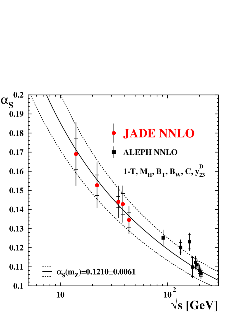
Figure 2: The values for $\alpha_{\mathrm{S}}$ at the JADE energy points. The inner error bars correspond to the combined statistical and experimental errors and the outer error bars show the total errors. The results from $\sqrt{s}=34.6$ and 35 GeV have been combined for clarity. The full and dashed lines indicate the result from our JADE NNLO analysis as shown on the figure. The results from the NNLO analysis of ALEPH data dissertori07 are shown as well.

A combination of the combined results at the six JADE energy points shown in table 5 after running to a common reference scale $m_{\mathrm{Z^{0}}}$ using the combination procedure described above results in

$$\alpha_{\mathrm{S}}(m_{\mathrm{Z^{0}}}) =0.1210 \pm 0.0007\mathrm{(stat.)}\pm 0.0021\mathrm{(exp.)}$$

$$\pm 0.0044\mathrm{(had.)}\pm 0.0036\mathrm{(theo.)}$$

($\alpha_{\mathrm{S}}(m_{\mathrm{Z^{0}}})=0.1210\pm 0.0061$) for the NNLO analysis and

$$\alpha_{\mathrm{S}}(m_{\mathrm{Z^{0}}}) =0.1172 \pm 0.0006\mathrm{(stat.)}\pm 0.0020\mathrm{(exp.)}$$

$$\pm 0.0035\mathrm{(had.)}\pm 0.0030\mathrm{(theo.)}$$

($\alpha_{\mathrm{S}}(m_{\mathrm{Z^{0}}})=0.1172\pm 0.0051$) for the NNLO+NLLA analysis. The NNLO+NLLA result has smaller hadronisation and theory uncertainties compared with the values in the NNLA analysis. We choose the latter result from NNLO+NLLA fits as our final result, because it is based on the most complete theory predictions and it has smaller theory uncertainties. It is consistent with the world average of $\alpha_{\mathrm{S}}(m_{\mathrm{Z^{0}}})=0.119\pm 0.001$ bethke06 , the recent NNLO analysis of event shape data from the ALEPH experiment $\alpha_{\mathrm{S}}(m_{\mathrm{Z^{0}}})=0.1240\pm 0.0033$ dissertori07 as well as with the related average of $\alpha_{\mathrm{S}}(m_{\mathrm{Z^{0}}})=0.120\pm 0.005$ from the analyses of the LEP experiments using NLO+NLLA QCD predictions kluth06 . The total error for $\alpha_{\mathrm{S}}(m_{\mathrm{Z^{0}}})$ of 4% is among the most precise determinations of $\alpha_{\mathrm{S}}(m_{\mathrm{Z^{0}}})$ currently available.

After running the fit results for $\alpha_{\mathrm{S}}(\sqrt{s})$ for each observable to the common reference scale $m_{\mathrm{Z^{0}}}$ we combine the results for a given observable to a single value. We use the same method as above and obtain the results for $\alpha_{\mathrm{S}}(m_{\mathrm{Z^{0}}})$ shown in table 6. The rms values of the results for $\alpha_{\mathrm{S}}(m_{\mathrm{Z^{0}}})$ are 0.0029 for the NNLO analysis and 0.0026 for the NNLO+NLLA analysis; both values are consistent with the errors of the corresponding combined results shown in equations (5.5) and (5.5). Figure 3 shows the combined results of $\alpha_{\mathrm{S}}(m_{\mathrm{Z^{0}}})$ for each observable together with results from alternative analyses discussed below. Combining the combined results for each observable or combining all individual results after evolution to the common scale $m_{\mathrm{Z^{0}}}$ yields results consistent with equation (5.5) within $\Delta\alpha_{\mathrm{S}}(m_{\mathrm{Z^{0}}})=0.0004$ and the uncertainties also agree.

The hadronisation uncertainty of $M_{\mathrm{H}}$ at each energy point and in the combinations shown in table 6 is the smallest. We have repeated the combinations without $M_{\mathrm{H}}$ and found results for $\alpha_{\mathrm{S}}(m_{\mathrm{Z^{0}}})$ consistent within 0.6% with our main results with hadronisation uncertainties increased by 14% (NNLO) or 20% (NNLO+NLLA).

Table 6: Combined values of $\alpha_{\mathrm{S}}(m_{\mathrm{Z^{0}}})$ for each observable from NNLO (upper section) and NNLO+NLLA (lower section) analyses together with the statistical, experimental, hadronisation and theory errors.

Obs.	$\alpha_{\mathrm{S}}(m_{\mathrm{Z^{0}}})$	$\pm$stat.	$\pm$exp.	$\pm$had.	$\pm$theo.
$1-T$	0.1196	0.0011	0.0028	0.0067	0.0049
$M_{\mathrm{H}}$	0.1266	0.0009	0.0047	0.0014	0.0040
$B_{\mathrm{T}}$	0.1190	0.0009	0.0023	0.0047	0.0055
$B_{\mathrm{W}}$	0.1232	0.0008	0.0034	0.0037	0.0035
$C$	0.1184	0.0013	0.0029	0.0081	0.0045
$y_{23}^{\mathrm{D}}$	0.1201	0.0005	0.0014	0.0046	0.0026
$1-T$	0.1175	0.0010	0.0026	0.0061	0.0041
$M_{\mathrm{H}}$	0.1210	0.0008	0.0037	0.0011	0.0032
$B_{\mathrm{T}}$	0.1151	0.0009	0.0019	0.0039	0.0042
$B_{\mathrm{W}}$	0.1143	0.0006	0.0026	0.0028	0.0026
$C$	0.1148	0.0011	0.0027	0.0073	0.0044
$y_{23}^{\mathrm{D}}$	0.1199	0.0005	0.0013	0.0046	0.0023

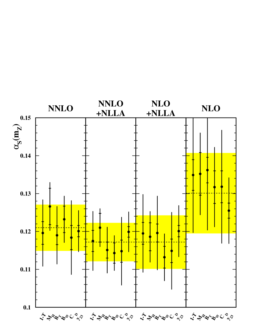
Figure 3: The combined results for $\alpha_{\mathrm{S}}(m_{\mathrm{Z^{0}}})$ for each type of analysis as indicated on the figure. The shaded bands and dashed lines show the combined values of $\alpha_{\mathrm{S}}(m_{\mathrm{Z^{0}}})$ with total errors. The inner and outer error bars show the combined statistical and experimental and the total errors.

In order to study the compatibility of our data with the QCD prediction for the evolution of the strong coupling with cms energy we repeat the combinations with or without evolution of the combined results to the common scale. We set the theory uncertainties to zero since these uncertainties are highly correlated between energy points. We conservatively assume the hadronisation uncertainties to be partially correlated, because these uncertainties depend strongly on the cms energy. The $\chi^{2}$ probabilities of the averages for running (not running) with NNLO+NLLA fits then become 0.39 ($9.9\cdot 10^{-3}$). With the NNLO fits the $\chi^{2}$ probabilities for running (not running) are 0.48 ($1.2\cdot 10^{-3}$). We interpret this as strong evidence for the dependence of the strong coupling on cms energy as predicted by QCD from JADE data alone.

5.6 Comparison with NLO and NLO+NLLA

For a comparison of our results with previous $\alpha_{\mathrm{S}}$ measurements the fits to the event shape distributions are repeated with NLO predictions and with NLO predictions combined with resummed NLLA with the modified $\ln R$-matching scheme (NLO+NLLA), both with $x_{\mu}=1$. The NLO+NLLA predictions with the modified $\ln R$-matching scheme were the standard of the final analysis of the LEP experiments l3290 ; aleph265 ; OPALPR404 ; delphi327 . The fit ranges as well as the procedures for evaluation of the systematic uncertainties are identical to the ones in our NNLO and NNLO+NLLA analyses.

The combination of the fits using NLO predictions returns $\alpha_{\mathrm{S}}(m_{\mathrm{Z^{0}}})=0.1301\pm 0.0009\mathrm{(stat.)}\pm 0.0029\mathrm{(exp.)}\pm 0.0054\mathrm{(had.)}\pm 0.0086\mathrm{(theo.)}$, the fits using combined NLO+ NLLA predictions yield $\alpha_{\mathrm{S}}(m_{\mathrm{Z^{0}}})=0.1172\pm 0.0007\mathrm{(stat.)}\pm 0.0022\mathrm{(exp.)}\pm 0.0039\mathrm{(had.)}\pm 0.0054\mathrm{(theo.)}$ and these results are shown in figure 3. The result obtained with the NLO+NLLA prediction is consistent with our NNLO and NNLO+NLLA analyses, but the theory uncertainties are larger by about 60%. The analysis using NLO predictions gives theoretical uncertainties larger by a factor of 2.6 and the value for $\alpha_{\mathrm{S}}(m_{\mathrm{Z^{0}}})$ is larger compared to the NNLO or NNLO+NLLA results. It has been observed previously that values for $\alpha_{\mathrm{S}}$ from NLO analysis with $x_{\mu}=1$ are large in comparison with most other analyses OPALPR054 . Both the NLO+NLLA or NNLO+NLLA analyses yield a smaller value of $\alpha_{\mathrm{S}}(m_{\mathrm{Z^{0}}})$ compared to the respective NLO or NNLO results. The difference between NNLO+NLLA and NNLO is smaller than the difference between NLO+NLLA and NLO, since a larger part of the NLLA terms is included in the NNLO predictions.

5.7 Renormalisation Scale Dependence

The theoretical uncertainty due to missing higher order terms is evaluated by setting the renormalisation scale parameter $x_{\mu}$ to 0.5 or 2.0. In order to assess the dependence of $\alpha_{\mathrm{S}}$ on the renormalisation scale the fits are repeated using NNLO, NNLO+NLLA, NLO and NLO+NLLA predictions with $0.1<x_{\mu}<10$. The strong coupling $\alpha_{\mathrm{S}}$ as well as the $\chi^{2}/\mathrm{d.o.f.}$ as a function of $x_{\mu}$ for $1-T$ at $\sqrt{s}=35$ GeV are shown in figure 4. The $\chi^{2}/\mathrm{d.o.f.}$ curves for the NLO+NLLA and NNLO+NLLA fits show no local minimum in the $x_{\mu}$ range studied. The $\alpha_{\mathrm{S}}(m_{\mathrm{Z^{0}}})$ values from NLO predictions are the largest for $x_{\mu}>0.2$. The $\alpha_{\mathrm{S}}(m_{\mathrm{Z^{0}}})$ values using NLO+NLLA and NNLO calculation almost cross at the natural choice of the renormalisation scale $x_{\mu}=1$ while the $\alpha_{\mathrm{S}}(m_{\mathrm{Z^{0}}})$ value from the NNLO+NLLA fit is slightly lower. The NLLA terms at $x_{\mu}=1$ are almost identical to the $\mathcal{O}(\alpha_{\mathrm{S}}^{3})$-terms in the NNLO calculation. A similar behaviour can be observed for $B_{\mathrm{T}}$ and $y_{23}^{\mathrm{D}}$. The slopes of the $\alpha_{\mathrm{S}}(m_{\mathrm{Z^{0}}})$ curves of the NNLO and NNLO+NLLA fits around the default choice $x_{\mu}=1$ are smaller than the slopes for the NLO and NLO+NLLA fits leading to the decreased theoretical uncertainties in our analyses.

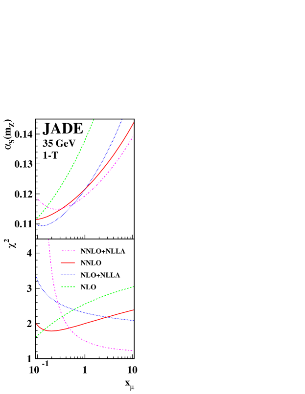
Figure 4: The plot shows the result of $\alpha_{\mathrm{S}}(m_{\mathrm{Z^{0}}})$ and $\chi^{2}$/d.o.f. of the fit to the thrust event shape distribution for $\sqrt{s}=35$ GeV.

6 Conclusion

In this paper we present measurements of the strong coupling $\alpha_{\mathrm{S}}$ using event shape observable distributions at cms energies $14<\sqrt{s}<44$ GeV. To determine $\alpha_{\mathrm{S}}$ fits using NNLO and combined NNLO+NLLA predictions were used. Combining the results from NNLO+NLLA fits to the six event shape observables $1-T$, $M_{\mathrm{H}}$, $B_{\mathrm{W}}$, $B_{\mathrm{T}}$, $C$ and $y_{23}^{\mathrm{D}}$at the six JADE energy points returns $\alpha_{\mathrm{S}}(m_{\mathrm{Z^{0}}})=0.1172\pm 0.0006\mathrm{(stat.)}\pm 0.0020\mathrm{(exp.)}\pm 0.0035\mathrm{(had.)}\pm 0.0030\mathrm{(theo.)}$, with a total error on $\alpha_{\mathrm{S}}(m_{\mathrm{Z^{0}}})$ of 4%. The investigation of the renormalisation scale dependence of $\alpha_{\mathrm{S}}(m_{\mathrm{Z^{0}}})$ shows a reduced dependence on $x_{\mu}$ when NNLO or NNLO+NLLA predictions are used, compared to analyses with NLO or NLO+NLLA predictions. The more complete NNLO or NNLO+NLLA QCD predictions thus lead to smaller theoretical uncertainties in our analysis. The combined results for $\alpha_{\mathrm{S}}$ at each cms energy are consistent with the running of $\alpha_{\mathrm{S}}$ as predicted by QCD and exclude absence of running with a confidence level of 99%.

References

-
(1)
J. Allisone,
K. Ambrusc,
J. Armitagee,
J. Bainese,
A.H. Balle,
G. Bamforde,
R. Barlowe,
W. Bartela,
L. Beckera,
A. Belld,
S. Bethkec,
C. Bowderyd,
T. Canzlera,
S.L. Cartwrightg,
J. Chrine,
D. Clarkeg,
D. Cordsa,
D.C. Darvilld,
A. Dieckmannc,
G. Dietrichb,
P. Dittmanna,
H. Drummc,
I.P. Duerdothe,
G. Eckerlinc,
R. Eichlera,
E. Elsenb,
R. Felsta,
A. Finchd,
F. Fosterd,
R.G. Glasserf,
I. Glendinninge,
M.C. Goddardg,
T. Greenshawe,
J. Hagemannb,
D. Haidta,
J.F. Hassarde,
R. Hedgecockg,
J. Heintzec,
G. Heinzelmannb,
G. Heinzelmannb,
K.H. Hellenbrandc,
M. Helmb,
R. Heuerc,
P. Hillf,
G. Hughesd,
M. Imorih,
H. Jungea,
H. Kadob,
J. Kanzakih,
S. Kawabataa,
K. Kawagoeb,
T. Kawamotoh,
B.T. Kinge,
C. Kleinwortb,
G. Kniesa,
T. Kobayashih,
S. Komamiyac,
M. Koshibah,
H. Krehbiela,
M. Kuhlenb,
P. Laurikainena,
P. Lennertc,
F.K. Loebingere,
A.A. Macbethe,
N. Magnussenb,
R. Marshallg,
T. Mashimoh,
H. Matsumurac,
H. McCanne,
K. Meierb,
R. Meinkea,
R.P. Middletong,
H.E. Millse,
M. Minowah,
P.G. Murphye,
B. Naroskaa,
T. Nozakid,
M. Nozakih,
J. Nyed,
S. Odakah,
T. Oestb,
J. Olssona,
L.H. O’Neilla,
S. Oritoh,
F. Ould-Saadab,
G.F. Pearceg,
A. Petersenb,
E. Pietarienena,
D. Pitzlb,
H. Prospere,
J.J. Pryced,
R. Pustb,
R. Ramckeb,
H. Riesebergc,
P. Rowee,
A. Satoh,
D. Schmidta,
U. Schneeklothb,
B. Sechi-Zornf,
J.A. Skardf,
L. Smolikc,
J. Spitzerc,
P. Steffena,
K. Stephense,
T. Sudah,
H. Takedah,
T. Takeshitah,
Y. Totsukah,
H. v.d.Schmittc,
J. von Kroghc,
A. Wagnerc,
S.R. Wagnerf,
I. Walkerd,
P. Warmingb,
Y. Watanabeh,
G. Weberb,
A. Wegnerb,
H. Wenningera,
J.B. Whittakerg,
H. Wriedtd,
S. Yamadah,
C. Yanagisawah,
W.L. Yena,
M. Zacharaa,
Y. Zhanga,
M. Zimmerc,
G.T. Zornf
a Deutsches Elektronen-Synchrotron DESY, Hamburg, Germany
b II. Institut für Experimentalphysik der Universität Hamburg, Germany
c Physikalisches Institut der Universität Heidelberg, Germany
d University of Lancaster, England
e University of Manchester, England
f University of Maryland, College Park, MD, USA
g Rutherford Appleton Laboratory, Chilton, Didcot, England
h International Center for Elementary Particle Physics, ICEPP, University of Tokyo, Tokyo, Japan - (2) O. Biebel, Phys. Rep. 340, 165 (2001)
- (3) M. Dasgupta, G.P. Salam, J. Phys. G 30, R143 (2004)
- (4) G. Dissertori, I.G. Knowles, M. Schmelling, Quantum Chromodynamics. International Series of Monographs on Physics number 115, Clarendon Press (2003), Oxford
- (5) S. Kluth, Rept. Prog. Phys. 69, 1771 (2006)
- (6) H. Fritzsch, Murray Gell-Mann, H. Leutwyler, Phys. Lett. B 47, 365 (1973)
- (7) D.J. Gross, Frank Wilczek, Phys. Rev. Lett. 30, 1343 (1973)
- (8) D.J. Gross, Frank Wilczek, Phys. Rev. D 8, 3633 (1973)
- (9) H.David Politzer, Phys. Rev. Lett. 30, 1346 (1973)
- (10) A. Gehrmann-De Ridder, T. Gehrmann, E.W.N. Glover, G. Heinrich, J. High Energy Phys. 12, 094 (2007)
- (11) T. Gehrmann, G. Luisoni, H. Stenzel, Phys. Lett. B 664, 265 (2008)
- (12) G. Dissertori et al., J. High Energy Phys. 02, 040 (2008)
- (13) R.A. Davison, B.R. Webber, Eur. Phys. J. C 59, 13 (2009)
- (14) B. Naroska, Phys. Rep. 148, 67 (1987)
- (15) JADE Coll., J. Schieck et al., Eur. Phys. J. C 48, 3 (2006), Erratum-ibid.C50:769,2007
- (16) T. Sjöstrand, Comput. Phys. Commun. 82, 74 (1994)
- (17) G. Marchesini et al., Comput. Phys. Commun. 67, 465 (1992)
- (18) L. Lönnblad, Comput. Phys. Commun. 71, 15 (1992)
- (19) OPAL Coll., G. Alexander et al., Z. Phys. C 69, 543 (1996)
- (20) OPAL Coll., G. Abbiendi et al., Eur. Phys. J. C 35, 293 (2004)
- (21) S. Brandt, Ch. Peyrou, R. Sosnowski, A. Wroblewski, Phys. Lett. 12, 57 (1964)
- (22) E. Fahri, Phys. Rev. Lett. 39, 1587 (1977)
- (23) T. Chandramohan, L. Clavelli, Nucl. Phys. B 184, 365 (1981)
- (24) S. Catani, G. Turnock, B.R. Webber, Phys. Lett. B 295, 269 (1992)
- (25) G. Parisi, Phys. Lett. B 74, 65 (1978)
- (26) J.F. Donoghue, F.E. Low, S.Y. Pi, Phys. Rev. D 20, 2759 (1979)
- (27) R.K. Ellis, D.A. Ross, A.E. Terrano, Nucl. Phys. B 178, 421 (1981)
- (28) OPAL Coll., M.Z. Akrawy et al., Phys. Lett. B 235, 389 (1990)
- (29) MARK II Coll., S. Komamiya et al., Phys. Rev. Lett. 64, 987 (1990)
- (30) S. Catani et al., Phys. Lett. B 269, 432 (1991)
- (31) S. Weinzierl, MZ-TH-08-22 (2008), 0807.3241
- (32) OPAL Coll., G. Alexander et al., Z. Phys. C 72, 191 (1996)
- (33) OPAL Coll., G. Abbiendi et al., Eur. Phys. J. C 40, 287 (2005)
- (34) R.K. Ellis, W.J. Stirling, B.R. Webber, QCD and Collider Physics. Vol. 8 of Cambridge Monographs on Particle Physics, Nuclear Physics and Cosmology, Cambridge University Press (1996)
- (35) R.W.L. Jones, M. Ford, G.P. Salam, H. Stenzel, D. Wicke, J. High Energy Phys. 12, 007 (2003)
- (36) P.A. Movilla Fernández, Ph.D. thesis, RWTH Aachen, 2003, PITHA 03/01
- (37) JADE Coll., O. Biebel, P.A. Movilla Fernández, S. Bethke et al., Phys. Lett. B 459, 326 (1999)
- (38) OPAL Coll., G. Abbiendi et al., Eur. Phys. J. C 53, 21 (2008)
- (39) R.W.L. Jones, Nucl. Phys. Proc. Suppl. 133, 13 (2004)
- (40) ALEPH Coll., A. Heister et al., Eur. Phys. J. C 35, 457 (2004)
- (41) S. Bethke, Prog. Part. Nucl. Phys. 58, 351 (2007)
- (42) L3 Coll., P. Achard et al., Phys. Rep. 399, 71 (2004)
- (43) DELPHI Coll., J. Abdallah et al., Eur. Phys. J. C 37, 1 (2004)
- (44) OPAL Coll., P.D. Acton et al., Z. Phys. C 55, 1 (1992)