Kinetics of Phase Separation in Thin Films: Lattice versus Continuum Models for Solid Binary Mixtures

Abstract

A description of phase separation kinetics for solid binary (A,B) mixtures in thin film geometry based on the Kawasaki spin-exchange kinetic Ising model is presented in a discrete lattice molecular field formulation. It is shown that the model describes the interplay of wetting layer formation and lateral phase separation, which leads to a characteristic domain size $\ell(t)$ in the directions parallel to the confining walls that grows according to the Lifshitz-Slyozov $t^{1/3}$ law with time $t$ after the quench. Near the critical point of the model, the description is shown to be equivalent to the standard treatments based on Ginzburg-Landau models. Unlike the latter, the present treatment is reliable also at temperatures far below criticality, where the correlation length in the bulk is only of the order of a lattice spacing, and steep concentration variations may occur near the walls, invalidating the gradient square approximation. A further merit is that the relation to the interaction parameters in the bulk and at the walls is always transparent, and the correct free energy at low temperatures is consistent with the time evolution by construction.

I Introduction

A basic problem of both materials science 1 ; 2 and statistical mechanics of systems out of equilibrium 2 ; 3 ; 4 ; 5 is the process of spinodal decomposition of binary (A,B) mixtures. When one brings the system by a sudden change of external control parameters (e.g., a temperature quench) from an equilibrium state in the one-phase region of the mixture to a state inside of the miscibility gap, thermal equilibrium requires coexistence of macroscopically large regions of A-rich and B-rich phases. Related phenomena also occur in systems undergoing order-disorder phase transitions, and it is also possible that an interplay of ordering and phase separation occurs, particularly in metallic alloys with complex phase diagrams 1 ; 2 ; 6 .

The recent interest in nanostructured materials and thin films has led to consider the effects of walls or free surfaces on the kinetics of such phase changes 7 ; 8 ; 9 ; 10 ; 11 ; 12 ; 13 ; 14 ; 15 ; 16 ; 17 ; 18 ; 19 . In a binary mixture, it is natural to expect that one of the components (say, A) will be preferentially attracted to the surface. Already in the one phase region, this attraction will lead to the formation of surface enrichment layers of the preferred component at the walls, but the thickness of these layers will be small, viz., of the order of the correlation length $\xi$ of concentration fluctuations in the mixture 20 . Only near the critical point this surface enrichment becomes long ranged 21 ; 22 . For temperatures below the critical point, however, the behavior is more complicated due to the interplay between bulk phase separation and wetting phenomena 23 ; 24 ; 25 ; 26 ; 27 ; 28 ; 29 . In a semi-infinite geometry, a B-rich domain of a phase separated mixture would be coated with an A-rich wetting layer at the surface, if the temperature is above the wetting transition. Of course, for thin films the finite film thickness $D$ also constrains the growth of wetting layers: E.g., for short range forces between the walls and the A-atoms the equilibrium thickness of a “wetting layer” is of the order of $\xi\ln(D/\xi)$ 29 ; 30 ; 31 , while at lower temperatures where the surface is nonwet the thickness of the surface enrichment layer again only is of the order of $\xi$. Also the phase diagram of the system in a thin film geometry differs from that of the bulk, in analogy to capillary condensation of fluids 29 ; 31 ; 32 ; 33 ; 34 , and very rich phase diagrams may occur, in particular, if the surfaces confining the thin film are not of the same type 29 ; 35 ; 36 ; 37 . These changes in the phase behavior of thin films are reflected in the kinetics of phase separation in these systems 18 ; 19 , of course.

Despite the large theoretical activity on surface effects on phase separation kinetics 8 ; 9 ; 10 ; 12 ; 13 ; 14 ; 15 ; 17 ; 18 ; 19 the applicability of these works on experiments is very restricted. Actually, most of the experiments deal with thin films of fluid binary mixtures 7 ; 11 ; 16 , but almost all theoretical works 8 ; 9 ; 10 ; 12 ; 13 ; 14 ; 15 ; 17 ; 18 deal with “model $B$” 38 , where hydrodynamic interactions are neglected, and hence this model is really appropriate only for solid mixtures.

A second restriction on the applicability of the theory is the fact that it is based on the time-dependent Ginzburg-Landau model 1 ; 2 ; 3 ; 4 ; 5 ; 6 , and thus is applicable only when the correlation length $\xi$ is very large, i.e. in the immediate vicinity of the bulk critical point. For a thin film with short range surface forces, the “standard model” is based on a free energy functional of an order parameter $\psi$, and this functional consists of a bulk term ($F_{\rm b}$) and two terms representing the two surfaces $\mathcal{S}1$, $\mathcal{S}2$ 8 ; 10 ; 12 ; 13 ; 14 ; 17 ; 18 , $F[\psi]=F_{\rm b}+F_{\mathcal{S}1}+F_{\mathcal{S}2}$, with

$$F_{\rm b}[\psi] = \int d\vec{r}\;\Big{\{}-\frac{\psi(\vec{r})^{2}}{2}+\frac{\psi(\vec{r})^{4}}{4}+\frac{1}{4}[\vec{\nabla}\psi(\vec{r})]^{2}\Big{\}},$$ (1)

$$F_{\mathcal{S}1} = \int\limits_{\mathcal{S}1}d\vec{\rho}\;\Big{\{}-\frac{g}{2}[\psi(\vec{\rho},0)]^{2}-h_{\mathcal{S}1}\psi(\vec{\rho},0)$$ (2)

$$-\gamma\psi(\vec{\rho},0)\frac{\partial\psi}{\partial z}|_{z=0}\Big{\}},$$

$$F_{\mathcal{S}2} = \int\limits_{\mathcal{S}2}d\vec{\rho}\;\Big{\{}-\frac{g}{2}[\psi(\rho,D)\big{]}^{2}-h_{\mathcal{S}2}\psi(\vec{\rho},D)$$ (3)

$$+\gamma\psi(\vec{\rho},D)\frac{\partial\psi}{\partial z}|_{z=D}\Big{\}}.$$

Here $\psi(\vec{r})$ is the order parameter which is proportional to the density difference between the two species; it is normalized such that the coexisting A-rich and B-rich bulk phases for temperature $T<T_{\rm cb}$ ($T_{\rm cb}$ being the bulk critical temperature) correspond to $\psi=\pm 1$, respectively. All lengths are measured in units of $2\xi$, with $\xi$ denoting the bulk correlation length at the coexistence curve. The terms $F_{\mathcal{S}1}$ and $F_{\mathcal{S}2}$ are the local contributions from the surfaces $\mathcal{S}1$ and $\mathcal{S}2$, which for a film of thickness $D$, are located at $z=0$ and $z=D$, respectively, orienting the $z$-axis perpendicular to the surfaces, while $\vec{\rho}$ denotes the $(d-1)$ coordinates parallel to the surfaces, $d$ being the dimensionality. In $F_{\mathcal{S}1}$ there are parameters $g,\gamma$, and $h_{\mathcal{S}1}$, which can be related to the temperature $T$ and various parameters of an Ising ferromagnet with a free surface at which a surface magnetic field $H_{\mathcal{S}1}$ acts 8 ; 39

$$h_{\mathcal{S}1} = 4(H_{\mathcal{S}1}/T)(\sqrt{12})^{3}\xi^{5}/\sqrt{3},$$

$$g = 8(4J_{s}/J-5)\xi^{4},$$

$$\gamma = 4\xi^{3},$$ (4)

with

$$\xi=\frac{1}{\sqrt{12}}\Big{[}1-\frac{T}{T_{\rm cb}}\Big{]}^{-1/2},\,\,k_{\rm B}T_{\rm cb}=6J.\quad$$ (5)

In Eqs. (I, 5), a simple cubic lattice was assumed, the $z$-axis coinciding with a lattice axis. Nearest neighbor Ising spins in the lattice interact with an exchange coupling $J$, except for the surface plane at $z=0$ where the exchange coupling is $J_{\mathcal{S}}$. For deriving Eqs. (1, 2) from a layerwise molecular field approximation, the limit $\xi\rightarrow\infty$ needs to be taken, with $\psi(\vec{\rho},z)=m_{n}(\vec{\rho},t)/m_{\rm b}$, where $n$ is the layer index of the lattice, $n=1$ being the surface plane, and $m_{\rm b}$ [$=\sqrt{3}(1-T/T_{\rm cb})^{1/2}$] the bulk magnetization (note that $m_{\rm b}\rightarrow 0$ in the considered limit). Finally, $F_{\mathcal{S}2}$ describes analogously, the surface free energy of the surface at $z=D$, with $h_{\mathcal{S}2}$ being related to the surface field $H_{\mathcal{S}2}$ analogously to Eq. (I). In Eq. (5), $\xi$ is measured in units of the lattice spacing $a$ of the molecular field lattice model, which often, for the sake of convenience, we set to 1.

Dynamics is associated to the model assuming that in the bulk the order parameter evolves according to the (nonlinear) Cahn-Hilliard equation 1 ; 2 ; 3 ; 4 ; 5 ; 6

$$\frac{\partial}{\partial\tau}\psi(\vec{r},\tau)=-\vec{\nabla}\cdot\vec{J}(\vec{r},\tau)=\vec{\nabla}\cdot\Big{[}\vec{\nabla}\Big{(}\frac{\delta F}{\delta\psi}\Big{)}\Big{]},\quad$$ (6)

while the surfaces amount to two boundary conditions each 20 , which can be written as

$$\tau_{0}\frac{\partial}{\partial\tau}\psi(\vec{\rho},0,\tau) = -\frac{\delta\mathcal{F}}{\delta\psi(\vec{\rho},0,\tau)}$$ (7)

$$= h_{\mathcal{S}1}+g\psi(\vec{\rho},0,\tau)+\gamma\frac{\partial\psi}{\partial z}|_{z=0},$$

$$J_{z}(\vec{\rho},0,\tau) = -\frac{\partial}{\partial z}\left[-\psi+\psi^{3}-\frac{1}{2}\nabla^{2}\psi\right]=0.$$ (8)

Equation (7) describes a non-conserved relaxation (“model A” 38 ) for the order parameter at the surface, $\tau_{0}$ setting the time scale. Since $\psi(\vec{\rho},0,\tau)$ relaxes much faster than the time scales of phase separation away from the surface, one may put $\tau_{0}=0$. The equations for $z=D$ are fully analogous to those for $z=0$. We emphasize that Eq. (6) can also be derived 40 from a continuum approximation to a molecular field approximation to a description of a Kawasaki kinetic Ising model 41 , and Eqs. (7, 8) can be derived from a Kawasaki model with a free surface as well 20 . However, it is clear that the model, Eqs. (6, 7, 8), can only represent the molecular field Kawasaki kinetic Ising model accurately when $\xi\gg$ one lattice unit. This fact was already discussed in 20 in the one-phase region, where the linearized molecular field equations on the lattice were solved to describe the kinetics of surface enrichment for $T>T_{\rm cb}$, and it was found that the lattice and continuum theories agree when approximations such as $\exp(-1/\xi)\simeq 1-1/\xi$ become valid.

Thus, the model Eqs. (6, 7, 8) can describe a solid binary mixture accurately near the bulk critical point only: far below $T_{\rm cb}$, terms of order $\psi^{6}$ and higher would be needed in Eq. (1) already, and when $\xi$ is of the order of the lattice spacing $a$, also higher order gradient terms $(\vec{\nabla}^{2}\psi)^{2}$ etc. would be required for an accurate continuum description. However, the numerical solutions of Eqs. (6, 7, 8) require anyway a discretization: Often a mesh size $\Delta x=\Delta y=\Delta z=1$ is used to solve these equations 8 ; 10 ; 12 ; 13 ; 14 ; 17 ; 18 . This essentially corresponds to a lattice with spacing $2\xi$, rather than the spacing $a$ of the underlying Ising lattice. Having in mind applications of the theory at temperatures that are not close to the critical point, however, $\xi$ is of the order of $1$.

Thus, it is plausible that one could solve with a comparable effort the original (nonlinear) molecular field equations for the Kawasaki kinetic Ising model on the lattice, that are underlying this theory. The advantage of such a treatment clearly would be that the model has a well-defined microscopic meaning at all temperatures. Near the critical temperature, the results of this treatment should become indistinguishable from the solution of Eqs. (6, 7, 8), of course.

The purpose of the present work is to show that indeed such a lattice mean field approach to spinodal decomposition in thin films (and in the bulk) is both feasible and efficient. In Sec. II, we present the discrete lattice analogue of Eqs. (1, 2, 3), and (6, 7, 8), following up on the work by Binder and Frisch 20 . In Sec. III, we present various numerical results for deep quenches (i.e., temperatures far below criticality) and discuss the resulting structure formation for a symmetric film, both in directions parallel and perpendicular to the walls. In Sec. IV, we present a comparison to the continuum approach, Eqs. (6, 7, 8). Finally, Sec. V summarizes our paper, containing also an outlook on simulations where the basic atomistic model is not a lattice model, as is the case for spinodal decomposition in fluid binary mixtures.

II Molecular Field Theory for the Kawasaki Kinetic Ising Model in a Thin Film

The system that is considered is the ferromagnetic Ising model with nearest neighbor exchange on the simple cubic lattice, described by the Hamiltonian

$$\mathcal{H} = -J\sum\limits_{\langle i,j\rangle\atop{\rm bulk}}S_{i}S_{j}-J_{s}\sum\limits_{\langle i,j\rangle\,\atop\mathcal{S}1,\mathcal{S}2}S_{i}S_{j}$$ (9)

$$-H\sum\limits_{i}S_{i}-H_{\mathcal{S}1}\sum\limits_{i\,\in\,\mathcal{S}1}S_{i}-H_{\mathcal{S}2}\sum\limits_{i\,\,\in\,\mathcal{S}2}S_{i}.\,\,$$

Here $S_{i}=\pm 1$, lattice sites are labeled by the index $i$, and the first sum runs over all nearest neighbor pairs except those in the surfaces $\mathcal{S}1$ and $\mathcal{S}2$. Note that now for a film of thickness $D$, the surfaces $\mathcal{S}1$ and $\mathcal{S}2$ are located at $n=1$ and $n=n_{\mbox{max}}=D+1$, $n$ being an index labeling the lattice planes in the $z$-direction perpendicular to the surfaces. Also note that all distances will be measured in units of the lattice constant $a$. The term $-H\sum\limits_{i}S_{i}$ describes the Zeeman energy, $H$ being the bulk magnetic field, and the sum runs over all sites of the lattice. It should be remembered that in the interpretation of the Ising model related to binary mixtures, spin up corresponding to $A$ and spin down to $B$, $H$ would correspond to a chemical potential difference between the species.

The molecular field equations for the local magnetization $m_{n}(\vec{\rho})=\langle S_{i}\rangle$ (we denote the index $i$ of a lattice site by the index $n$ of the plane to which it belongs and a coordinate $\vec{\rho}$ in this plane) become 20

$$m_{n}(\vec{\rho}) = \tanh\frac{J}{k_{\rm B}T}\Big{[}m_{n+1}(\vec{\rho})+m_{n-1}(\vec{\rho})$$ (10)

$$+\sum_{\Delta\vec{\rho}}m_{n}(\vec{\rho}+\Delta\vec{\rho})+\frac{H}{J}\Big{]},\quad 2\leq n\leq D,$$

$$m_{1}(\vec{\rho}) = \tanh\frac{J}{k_{\rm B}T}\Big{[}m_{2}(\vec{\rho})+\frac{J_{S}}{J}\sum\limits_{\Delta\vec{\rho}}m_{1}(\vec{\rho}+\Delta\vec{\rho})$$ (11)

$$+\frac{H_{\mathcal{S}1}+H}{J}\Big{]},\quad n=1,$$

$$m_{D+1}(\vec{\rho}) = \tanh\frac{J}{k_{\rm B}T}\Big{[}m_{D}(\vec{\rho})+\frac{J_{S}}{J}\sum\limits_{\Delta\vec{\rho}}m_{D+1}(\vec{\rho}+\Delta\vec{\rho})$$ (12)

$$+\frac{H_{\mathcal{S}2}+H}{J}\Big{]},\quad n=D+1.\,$$

Here $\Delta\vec{\rho}$ is a vector connecting site $i$ with one of its 4 nearest neighbors in a layer. In the bulk, Eq. (10) reduces to the well-known transcendental equation

$$m_{\rm b}=\tanh[\frac{J}{k_{\rm B}T}(6m_{\rm b}+H/J)],$$ (13)

from which $T_{\rm cb}=6J/k_{\rm B}$ straightforwardly follows.

We also note that Eqs. (10,11,12) correspond to the free energy

$$F=\sum\limits^{D+1}_{n=1}(E_{n}-TS_{n})$$ (14)

with

$$\frac{S_{n}}{k_{\rm B}T} = \sum\limits_{\vec{\rho}}\Big{\{}\Big{(}\frac{1+m_{n}(\vec{\rho})}{2}\Big{)}\ln\Big{(}\frac{1+m_{n}(\vec{\rho})}{2}\Big{)}$$ (15)

$$+\frac{1-m_{n}(\vec{\rho})}{2}\ln\Big{(}\frac{1-m_{n}(\vec{\rho})}{2}\Big{)}\Big{\}},$$

$$E_{n} = -\sum\limits_{\vec{\rho}}\Big{\{}m_{n}(\vec{\rho})H+\frac{J}{2}m_{n}(\vec{\rho})(m_{n-1}(\vec{\rho})+m_{n+1}(\vec{\rho}))$$ (16)

$$+\frac{1}{2}Jm_{n}(\vec{\rho})\sum\limits_{\Delta\vec{\rho}}m_{n}(\vec{\rho}+\Delta\vec{\rho})\Big{\}},\quad 2\leq n\leq D,$$

$$E_{1} = -\sum\limits_{\vec{\rho}}\{m_{1}(\vec{\rho})(H+H_{1})+\frac{1}{2}Jm_{1}(\vec{\rho})m_{2}(\vec{\rho})$$ (17)

$$+\frac{1}{2}J_{S}m_{1}(\vec{\rho})\sum\limits_{\Delta\vec{\rho}}m_{1}(\vec{\rho}+\Delta\vec{\rho})\Big{\}},\quad n=1,$$

$$E_{D+1} = -\sum\limits_{\vec{\rho}}\Big{\{}m_{D+1}(\vec{\rho})(H+H_{\mathcal{S}2})+\frac{J}{2}m_{D+1}(\vec{\rho})m_{D}(\vec{\rho})$$ (18)

$$+\frac{J_{\mathcal{S}}}{2}m_{D+1}(\vec{\rho})\sum\limits_{\Delta\vec{\rho}}(\vec{\rho}+\Delta\vec{\rho})\Big{\}},\quad n=D+1.$$

Of course, Eqs. (10, 11, 12) can be derived from Eq. (14) via

$$\Big{(}\frac{\partial F}{\partial m_{n}(\vec{\rho})}\Big{)}_{T,H,H_{1},\{m_{n}(\vec{\rho})\}^{\prime}}=0$$ (19)

The prime on $\{m_{n}(\vec{\rho})\}^{\prime}$ indicates that all local magnetizations are held constant except the one that appears in the considered derivative. Of course, in equilibrium there is no explicit dependence on $\vec{\rho}$, although there clearly is a dependence on $n$.

However, already in equilibrium the $\vec{\rho}$-dependence is useful, when it is understood that the bulk field has a $\vec{\rho}$-dependence. Considering a wave vector dependent bulk field, one then can derive from Eq. (10) for $D\rightarrow\infty$ the wave vector dependent susceptibility $\chi(\vec{k})$. By linear response to the wave vector dependent field one finds, as is well-known,

$$\chi(\vec{k})=\frac{1}{k_{\rm B}T}\;\frac{1-m_{\rm b}^{2}}{1-[J(\vec{k})/k_{\rm B}T](1-m_{\rm b}^{2})},\quad$$ (20)

where $J(\vec{k})$ is the Fourier transform of the exchange interaction, i.e., in our case

$$J(\vec{k})=2J[\cos(k_{x}a)+\cos(k_{y}a)+\cos(k_{z}a)]\simeq 6J-Jk^{2}a^{2}.\,$$ (21)

From Eqs. (20, 21) we readily see that

$$\chi(\vec{k})=\chi(0)/[1+k^{2}\xi^{2}a^{2}],\quad\chi(0)=1/\Big{[}\frac{k_{\rm B}T}{1-m_{\rm b}^{2}}-k_{\rm B}T_{\rm cb}\Big{]}$$ (22)

and

$$\xi^{2}=\frac{J}{\frac{k_{\rm B}T}{1-m^{2}_{b}}-k_{\rm B}T_{\rm cb}}.$$ (23)

Equation (23) reduces to the result quoted in Eq. (5) when $T\rightarrow T_{\rm cb}$, but also shows that $\xi\rightarrow 0$ when $T\rightarrow 0$.

As discussed in 20 , we associate dynamics to the Ising model via the Kawasaki spin exchange model 41 , considering exchanges between nearest neighbors only. Following the method of 40 , one obtains with the help of the Glauber 42 transition probability a set of coupled kinetic equations for the local time-dependent mean magnetizations $\langle S_{i}(t)\rangle\equiv m_{n}(\vec{\rho},t)$ from the (exact) master equation 41 in molecular field approximation. Denoting the time scale in the transition probability as $\tau_{S}$, this set of equations is:

• $3\leq n\leq D-1$ (bulk case)

  $$2\tau_{S}\frac{d}{dt}m_{n}(\vec{\rho},t)=-6m_{n}(\vec{\rho},t)$$

  $$+m_{n-1}(\vec{\rho},t)+m_{n+1}(\vec{\rho},t)$$

  $$+\sum\limits_{\Delta\vec{\rho}}m_{n}(\vec{\rho}+\Delta\vec{\rho},t)$$

  $$+[1-m_{n}(\vec{\rho},t)m_{n-1}(\vec{\rho},t)]\tanh\frac{J}{k_{\rm B}T}[m_{n+1}(\vec{\rho},t)$$

  $$+m_{n-1}(\vec{\rho},t)+\sum\limits_{\Delta\vec{\rho}}m_{n}(\vec{\rho}+\Delta\vec{\rho},t)$$

  $$-m_{n}(\vec{\rho},t)-m_{n-2}(\vec{\rho},t)-\sum\limits_{\Delta\vec{\rho}}m_{n-1}(\vec{\rho}+\Delta\vec{\rho},t)]$$

  $$+[1-m_{n}(\vec{\rho},t)m_{n+1}(\vec{\rho},t)]\tanh\frac{J}{k_{\rm B}T}[m_{n+1}(\vec{\rho},t)$$

  $$+m_{n-1}(\vec{\rho},t)+\sum\limits_{\Delta\vec{\rho}}m_{n}(\vec{\rho}+\Delta\vec{\rho},t)-m_{n}(\vec{\rho},t)$$

  $$-m_{n+2}(\vec{\rho},t)-\sum\limits_{\Delta\vec{\rho}}m_{n+1}(\vec{\rho}+\Delta\vec{\rho},t)]$$

  $$+\sum\limits_{\Delta\vec{\rho}}[1-m_{n}(\vec{\rho},t)m_{n}(\vec{\rho}+\Delta\vec{\rho},t)]$$

  $$\tanh\frac{J}{k_{\rm B}T}[m_{n+1}(\vec{\rho},t)+m_{n-1}(\vec{\rho},t)+$$

  $$\sum\limits_{\Delta\vec{\rho}\;^{\prime}}m_{n}(\vec{\rho}+\Delta\vec{\rho}\;^{\prime},t)-m_{n+1}(\vec{\rho}+\Delta\vec{\rho},t)$$

  $$-m_{n-1}(\vec{\rho}+\Delta\vec{\rho},t)$$

  $$-\sum\limits_{\Delta\vec{\rho}\;^{\prime}}m_{n}(\vec{\rho}+\Delta\vec{\rho}+\Delta\vec{\rho}\;^{\prime},t)].$$ (24)

  Factors such as $[1-m_{n}m_{n-1}]$ arise from the mean field approximations to factors $(1-S_{i}S_{j})$ that express the fact that an exchange of $S_{i}$ with $S_{j}$ changes the magnetization $S_{i}$ only if $S_{i}$ and $S_{j}$ are oppositely oriented. In Eq. ((i)), exchanges of a spin at site $\vec{\rho}$ in layer $n$ with spins in layers $n-1$, $n+1$, and the same layer $n$ need to be considered. In the argument of the $\tanh$ functions, the difference of the effective fields acting on the spins that are exchanged is found. One can verify that Eq. ((i)) reduces to Eq. (10) if $dm_{n}(\vec{\rho},t)/dt=0$ is assumed: in equilibrium, the exchange of a spin with another one is exactly compensated by the inverse process. The kinetic equations near the wall are similar; one has to consider that in layer 1 a field $H_{\mathcal{S}1}$ is acting, and that no spin exchange into the layer $n=0$ (the wall) is possible. Hence, for

• $n=2$

  $$~{}~{}~{}2\tau_{S}\frac{d}{dt}m_{2}(\vec{\rho},t)=-6m_{2}(\vec{\rho},t)+m_{1}(\vec{\rho},t)$$

  $$+m_{3}(\vec{\rho},t)+\sum\limits_{\Delta\vec{\rho}}m_{2}(\vec{\rho}+\Delta\vec{\rho},t)$$

  $$+[1-m_{2}(\vec{\rho},t)m_{1}(\vec{\rho},t)]\tanh\frac{J}{k_{\rm B}T}[m_{3}(\vec{\rho},t)$$

  $$+m_{1}(\vec{\rho},t)+\sum\limits_{\Delta\vec{\rho}}m_{2}(\vec{\rho}+\Delta\vec{\rho},t)$$

  $$-\frac{H_{\mathcal{S}1}}{J}-m_{2}(\vec{\rho},t)-\frac{J_{S}}{J}\sum\limits_{\Delta\vec{\rho}}m_{1}(\vec{\rho}+\Delta\vec{\rho},t)]$$

  $$+[1-m_{2}(\vec{\rho},t)m_{3}(\vec{\rho},t)]\tanh\frac{J}{k_{\rm B}T}[m_{3}(\vec{\rho},t)+m_{1}(\vec{\rho},t)$$

  $$+\sum\limits_{\Delta\vec{\rho}}m_{2}(\vec{\rho}+\Delta\vec{\rho},t)$$

  $$-m_{4}(\vec{\rho},t)-m_{2}(\vec{\rho},t)-\sum\limits_{\Delta\vec{\rho}}m_{3}(\vec{\rho}+\Delta\vec{\rho},t)]$$

  $$+\sum\limits_{\Delta\vec{\rho}}[1-m_{2}(\vec{\rho},t)m_{2}(\vec{\rho}+\Delta\vec{\rho},t)]$$

  $$\tanh\frac{J}{k_{\rm B}T}[m_{3}(\vec{\rho},t)+m_{1}(\vec{\rho},t)+\sum\limits_{\Delta\vec{\rho}}m_{2}(\vec{\rho}+\Delta\vec{\rho},t)]$$

  $$-m_{3}(\vec{\rho}+\Delta\vec{\rho},t)-m_{1}(\vec{\rho}+\Delta\vec{\rho},t)$$

  $$-\sum\limits_{\Delta\vec{\rho}\;^{\prime}}m_{2}(\vec{\rho}+\Delta\vec{\rho}+\Delta\vec{\rho}\;^{\prime},t),$$ (25)

  and for

• $n=1$ (now only 5 neighbors are available for an exchange)
  

  $$2\tau_{S}\frac{d}{dt}m_{1}(\vec{\rho},t)=-5m_{1}(\vec{\rho},t)+m_{2}(\vec{\rho},t)$$

  $$+\sum\limits_{\Delta\vec{\rho}}m_{1}(\vec{\rho}+\Delta\vec{\rho},t)+$$

  $$[1-m_{1}(\vec{\rho},t)m_{2}(\vec{\rho},t)]\tanh\frac{J}{k_{\rm B}T}[m_{2}(\vec{\rho},t)$$

  $$+\frac{H_{\mathcal{S}1}}{J}+\frac{J_{\mathcal{S}}}{J}\sum\limits_{\Delta\rho}m_{1}(\vec{\rho}+\Delta\vec{\rho},t)$$

  $$-m_{3}(\vec{\rho},t)-m_{1}(\vec{\rho},t)-\sum\limits_{\Delta\vec{\rho}}m_{2}(\vec{\rho}+\Delta\vec{\rho},t)]+$$

  $$\sum\limits_{\Delta\vec{\rho}}[1-m_{1}(\vec{\rho},t)m_{1}(\vec{\rho}+\Delta\vec{\rho},t)]$$

  $$\tanh\frac{J}{k_{\rm B}T}[m_{2}(\vec{\rho},t)+\frac{J_{\mathcal{S}}}{J}\sum\limits_{\Delta\vec{\rho}\;^{\prime}}m_{1}(\vec{\rho}+\Delta\vec{\rho}\;^{\prime},t)$$

  $$-m_{2}(\vec{\rho}+\Delta\vec{\rho},t)-\frac{J_{\mathcal{S}}}{J}\sum\limits_{\Delta\vec{\rho}\;^{\prime}}m_{1}(\vec{\rho}+\Delta\vec{\rho}\;^{\prime}+\Delta\vec{\rho},t)].\quad$$ (26)

The equations for $n=D$ and $n=D+1$ are analogous. The time $t$ in Eqs. ((i), (ii), (iii)) is related to time $\tau$ in Eqs. (6, 7, 8) via

$$\tau=\frac{T_{\rm cb}/T-1}{8\tau_{s}\xi^{2}}.$$ (27)

The numerical solutions of the set of equations ((i), (ii), (iii)) for quenching experiments from infinite temperature to the states inside the miscibility gap is the subject of the next section.

III Numerical Results for Phase Separation following Deep Quenches

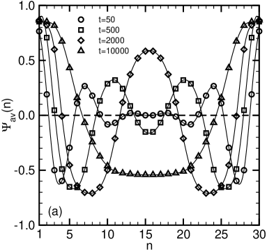
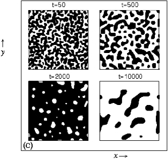
Figure 1: (a) Layerwise order parameter $\Psi_{av}(n)$ plotted vs. layer index $n$ for four different times for the choice $D=29,L=128$, and $H_{\mathcal{S}1}=H_{\mathcal{S}2}=1.0$. The continuous lines are cubic interpolations to the original data, used as guides to the eye. (b) Cross-sectional snapshot pictures of the same systems as in (a), displaying the magnetization configuration in the $xz$-plane for $y=L/2$. If the magnetization at a lattice site is positive, a black dot is printed. (c) Same as (b), but for a plane parallel to the walls, at $n=15$.

In this section we shall present selected results from the numerical solutions of Eqs. ((i), (ii), (iii)), choosing three values of the thickness of the film ($D=9$, 19, and 29, corresponding to $n_{\mbox{max}}=10$, 20, and 30 lattice planes, respectively), and a quench at time $t=0$ from infinite temperature to $T/T_{\rm cb}=2/3$, for the special cases $H_{\mathcal{S}1}=H_{\mathcal{S}2}=1.0$, 0.1, and $J_{\mathcal{S}}=J$. The initial conditions for $m_{n}(\vec{\rho},t)$ is chosen by taking $m_{n}(\vec{\rho},0)$ from a random uniform distribution between $-1$ and $+1$, with the total magnetization in the thin film zero.

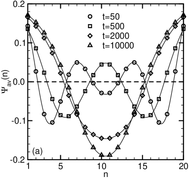
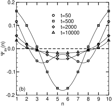
Figure 2: Layerwise average order parameter $\Psi_{\rm av}(n)$ plotted vs. $n$ for four different times for the cases (a) $D=19,L=128$ and (b) $D=9,L=128$. Always $H_{\mathcal{S}1}=H_{\mathcal{S}2}=0.1$ is chosen.

At first sight a quench to $T/T_{\rm cb}=2/3$ does not look like a particularly deep quench. However, one must keep in mind that in order to have $\xi$ larger (or equal) than a lattice spacing one must have $T\geq 5.57J/k_{\rm B}$, i.e. much closer to $T_{\rm cb}=6J/k_{\rm B}$. At the present temperature $k_{\rm B}T/J=4.0$, the correlation length is as small as $\xi\simeq 0.33$ lattice spacings. Following the standard reasoning for the simulation of the Ginzburg-Landau model, Eqs. (6, 7, 8), one should choose $2\xi$ as the size of the spatial discretization mesh: dealing with the above physical film thickness would require rather huge lattices. In addition, Eqs. (1, 2,3) do not represent the actual free energies of the lattice model [Eqs. (14, 15, 16, 17, 18)] accurately at such low temperatures either.

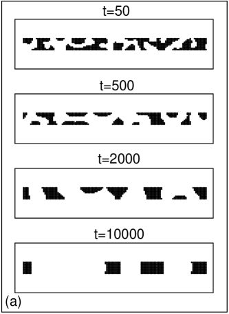
Figure 3: Cross-sectional snapshot pictures of the system with $D=9,L=128,H_{\mathcal{S}1}=H_{\mathcal{S}2}=0.1$ for (a) the $xz$-plane and (b) the $xy$-plane at $n=5$ for the same system as in Fig. 2(b).

Choosing the time unit $\tau_{s}=1$ in Eqs. ((i), (ii), (iii)) we have found that accurate numerical solutions of these equations result already when one chooses a rather large discrete time step, $\delta t=0.1$. Other than this discretization of time no approximations whatsoever enter the numerical solution. Of course, one always has to deal with a finite system geometry also in lateral directions: unless otherwise mentioned we choose $L_{x}=L_{y}=L=128$ for all values of $D$ and apply periodic boundary conditions in both the directions.

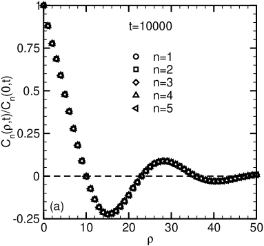
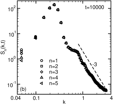
Figure 4: (a) Layerwise correlation function $C_{n}(\rho,t)$ plotted vs. $\rho$, for the choice $H_{\mathcal{S}1}=H_{\mathcal{S}2}=0.1$, $D=9,L=128,t=10000.$ Data for $n=1,2,3,4$ and 5 superimpose almost exactly. (b) Fourier transform $S_{n}(k,t)$ of $C_{n}(\rho,t)$, again resolved with respect to individual layers. In (b) the dashed line corresponds to the Porod tail $k^{-3}$.

Figure 1 shows data for a typical time evolution for $D=29$ and $H_{\mathcal{S}1}=H_{\mathcal{S}2}=1.0$. In Fig. 1(a), we show the layerwise average order parameter, $\Psi_{\rm av}(n)=L^{-2}\sum\limits_{\vec{\rho}}m_{n}(\vec{\rho},t)$, as a function of the layer index $n$. One sees that in the surface planes the magnetization takes its saturation value rather fast, as expected due to the large surface fields. Then the magnetization decreases very rapidly, already for $n=3$ the magnetization for $t=50$ is strongly negative. For $t=50$ the curve $\Psi_{\rm av}(n)$ then exhibits the oscillations typical for “surface-directed spinodal decomposition” 7 ; 8 ; 9 ; 10 ; 11 ; 12 ; 13 ; 14 ; 15 ; 16 ; 17 ; 18 ; 19 , with a second maximum at $n=7$ and a (weak) third one at $n=13$. Because of the symmetric surface fields, it is expected that the profile should be symmetric around the center of the film,

$$\Psi_{\rm av}(n)=\Psi_{\rm av}(D-n+2).\quad$$ (28)

But in reality this is not obeyed because of finite system size and lack of averaging over sufficiently large number of independent initial configurations (in our case averaging was done only over $5$ independent random initial configurations). However, all plots for $\Psi_{\rm av}(n)$ have been symmetrized by hand by taking advantage of property (28).

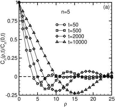
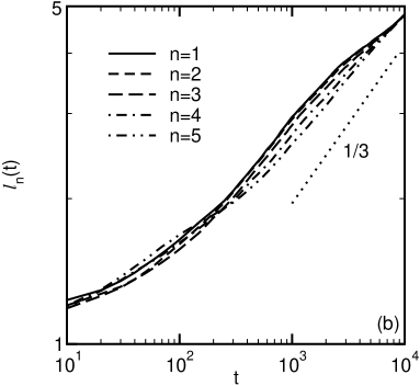
Figure 5: (a) Same as Fig. 4(a) but only for $n=5$, and four times as indicated. (b) Characteristic domain length $\ell_{n}(t)$ of individual layers, shown on a log-log plot versus time $t$. The dotted line corresponds to LS growth law $t^{1/3}$.

One can further see from Fig. 1(a) that the thickness of the surface enrichment layers at the walls slowly grows with increasing time, which is also obvious from Fig. 1(b) where we present the snapshot pictures of vertical sections ($xz$ plane). At a later time the position of the second peak of $\Psi_{\rm av}(n)$ has moved towards the center (it now occurs at $n=11$ for $t=500$) with a pronounced minimum in the center of the film. However, for $t\geq 2000$ this second peak has merged with its mirror image, i.e., now in the film center there is a maximum of $\Psi_{\rm av}(n)$ rather than a minimum. At very late time, this central maximum has disappeared again ($t=10000)$ and the profile looks like that of a simple stratified structure. Actually this is not the case, as seen in Fig. 1(c), where we have shown the snapshot pictures parallel to the surfaces ($xy$ plane) for $n=15$. As is also observed in the Ginzburg-Landau studies of surface-directed spinodal decomposition 8 ; 9 ; 10 ; 12 ; 13 ; 14 ; 17 ; 18 , in the lateral directions one can observe initially a rather random pattern which rapidly coarsens with increasing time.

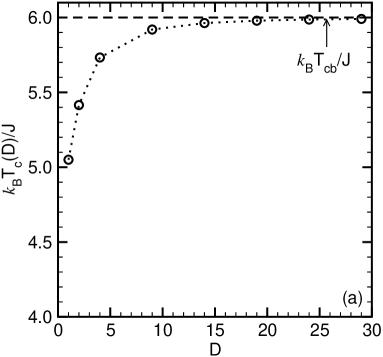
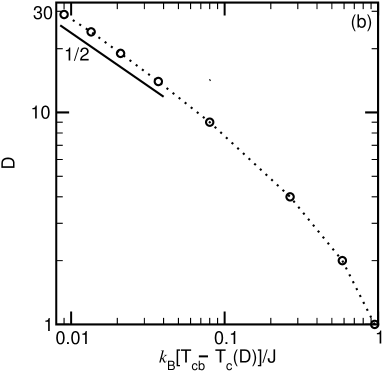
Figure 6: Plot of finite-size critical temperature $T_{c}(D)$ versus film thickness $D$, (a) on a linear scale and (b) on a log-log plot to display the asymptotic behavior $T_{\rm cb}-T_{\rm c}(D)\propto D^{-2}$ of mean field theory. The dashed line in (a) marks the bulk critical temperature, whereas the continuous line in (b) corresponds to the asymptotic theoretical prediction.

Figure 2 shows other examples where we have chosen thinner films (viz., $D=9$ and $D=19$) and a much weaker boundary field $(H_{\mathcal{S}1}=H_{\mathcal{S}2}=0.1)$. Now the amplitude of the variation of $\Psi_{\rm av}(n)$ is much smaller, and at late times the order parameter profiles across the film have almost no structure. The explanation for this behavior is seen in Fig. 3 where we show snapshot pictures of the states evolving for the choice $D=9$ of Fig. 2(b): The system develops towards a two-dimensional arrangement of columns of positive magnetization connecting the two walls, and thus in each plane ($n=\textrm{const}$), there is only a weak excess of magnetization in any one direction. These results qualitatively do not differ from the numerical studies of spinodal decomposition in thin films based on the Ginzburg-Landau equation, such as 18 ; however, the advantage of the present treatment is that the parameters of the model have an immediate and straightforward physical meaning. The fact that in the late stages there is almost no nontrivial structure across the film is also evident from a comparison of the pair correlation function $C_{n}(\rho,t)$ [$=\langle m_{n}(\vec{0},t)m_{n}(\vec{\rho},t)\rangle-\langle m_{n}(\vec{0},t)\rangle\langle m_{n}(\vec{\rho},t)\rangle$] and their Fourier transforms $S_{n}(k,t)$ in different layers, shown in Fig. 4.

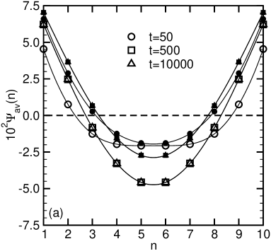
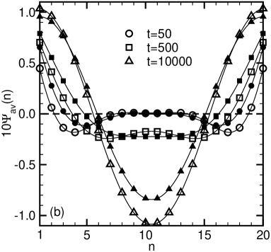
Figure 7: Comparison of the layerwise average order parameter profiles across the film for three times $(t=50,500$ and 10000, respectively), according to the lattice model (open symbols) and the GL model (filled symbols), for (a) $D=9$, and (b) $D=19$, respectively. All data refer to the choice $H_{\mathcal{S}1}=H_{\mathcal{S}2}=0.1,\;k_{\rm B}T/J=5.875$.

In Fig. 5(a), the plot of the time evolution of $C_{n}(\rho,t)$, for $n=5$, for the same system as in Fig. 3, clearly reflects the coarsening behavior. Note that the apparent nonscaling behavior of $C_{n}(\rho,t)$ is due to strong fluctuation of the layerwise average order parameter at early time. In Fig. 5(b) we plot the layerwise average domain size $\ell_{n}(t)$ as a function of $t$ extracted from the condition $C_{n}(\rho=\ell_{n}(t),t)=C_{n}(0,t)/2$. The characteristic length $\ell_{n}(t)$ initially grows rather slowly, for times $10<t<1000$ there is considerable curvature on the log-log plot, while for $t\geq 1000$ the behavior is already close to the standard Lifshitz-Slyozov (LS) 43 $\ell(t)\propto t^{1/3}$ law. The fact that the “effective exponent” $d[\ln\ell(t)]/d(\ln t)$ approaches 1/3 from below is quite reminiscent of Monte Carlo simulations of coarsening in the two-dimensional Kawasaki spin-exchange model 44 , of course. It should be noted that Monte Carlo simulations include thermal fluctuations that are absent in our molecular field treatment. However, it is generally believed 4 that thermal fluctuations are irrelevant during the late stages of coarsening. In view of these facts, the similarity of our results with the previous Monte Carlo studies of coarsening on lattice models is not unexpected. The advantage of the present approach in comparison with Monte Carlo, however, is that much less numerical effort is needed.

IV The Critical Region: A Comparison between the Lattice Approach and the Ginzburg-Landau treatment

Near the critical point one must take into account that the critical point is slightly shifted to lower temperatures for films of finite thickness as compared to the bulk 21 ; 31 ; 32 ; 33 ; 34 . In Fig. 6(a), we plot the critical temperatures, $T_{\rm c}(D)$, for films of finite width as a function of width $D$. The numerical values for $T_{\rm c}(D)$ were obtained by solving Eqs. (10, 11, 12) for $H=H_{\mathcal{S}1}=H_{\mathcal{S}2}=0$ starting with the assignment of uniform magnetization to the layers in a random fashion so that the total film magnetization is zero. Note that as $D\rightarrow\infty$, $T_{\rm c}(D)$ is expected to approach its $3$-$d$ mean field value $6J/k_{\rm B}=T_{\rm cb}$ and in the limit $D\rightarrow 0$, we expect the $2$-$d$ value $4J/k_{\rm B}$. In Fig. 6(b), we present the deviation of $T_{\rm c}(D)$ from $T_{\rm cb}$ as a function of $D$ on a log-log plot. From finite-size scaling theory, this difference should vanish as $T_{\rm cb}-T_{\rm c}(D)\sim D^{-2}$.

While for $D=29$ we have $T_{\rm c}(D)\simeq 5.99J/k_{\rm B}$, for $D=9$ we have $T_{\rm c}(D)\simeq 5.92J/k_{\rm B}$. Since lateral phase separation occurs only for $T<T_{\rm c}(D)$ 35 ; 36 ; 37 , of course, this shift restricts the range of $\xi$ that can be studied for the present choices of $D$. While $2\xi\simeq 1.0$ occurs for $T=4.75J/k_{\rm B}$ and hence this choice, for which the cell size of the Ginzburg Landau model agrees with the lattice spacing of the molecular field model, is safely accessible, already for $\xi\simeq 2.0$ (occurring for $k_{\rm B}T=5.875J$) we are only slightly below $T_{\rm c}(D=9)$, and for $\xi=3$ we would already be in the one-phase region of such a thin film. In view of these considerations, $k_{\rm B}T=5.875J$ was chosen as a temperature where it makes sense to compare the lattice model with $D=9$, 19, and 29 (i.e., $n_{\mbox{max}}=10$, 20, and 30 lattice planes, respectively) with the corresponding Ginzburg Landau (GL) model. Note that for the convenience of comparison as well as accuracy of numerical solutions, the discrete mesh sizes $\Delta x$, $\Delta y$, and $\Delta z$ in the GL model were adjusted to the lattice constant $a$ and we have set $\tau_{0}=0$.

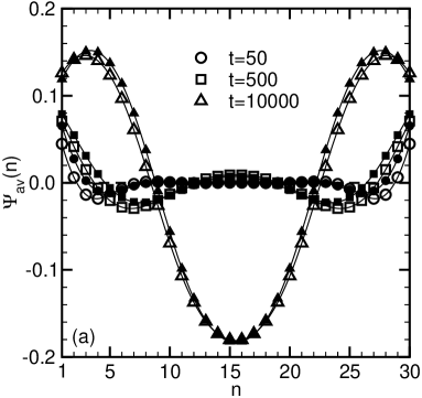
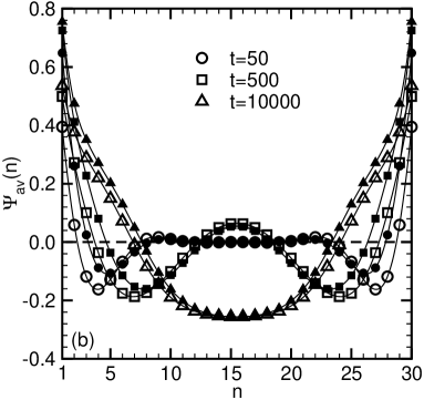
Figure 8: Same as Fig. 7, but for $D=29$, and two choices of the strength of the surface fields, $H_{\mathcal{S}1}=H_{\mathcal{S}2}=0.1$ (a) and $1.0$ (b).

In Fig. 7 we present the comparison between the lattice model and GL model at $k_{\rm B}T=5.875J$ ($\xi\simeq 2.0$, $m_{\rm b}\simeq 0.25$) with $H_{\mathcal{S}1}=H_{\mathcal{S}2}=0.1$ for $D=9$ and $19$. At this temperature the parameters $h_{\mathcal{S}1}$, $g$, $\gamma$, $\tau$ have the values $52.3$ ($523H_{\mathcal{S}1}$), -128, 32, and $t/1600$, respectively. One sees that for $D=9$ [Fig. 7(a)] the behavior of the lattice model and the GL model are qualitatively similar, but there is no quantitative agreement. These discrepancies do get smaller, however, with increasing film thickness [Fig. 7(b)]. In Fig. 8, where we plot the order parameter profile for D = 29 corresponding to two values of surface fields (see caption for details), we see that the discrepancies between the lattice and GL models are already quite small, irrespective of the choice of the surface field. However, for stronger surface field [Fig. 8(b)], the discrepancy is still visible at the surfaces. We expect that the comparison should be perfect for any surface field in the semi-infinite limit. In the immediate vicinity of the critical point, the close correspondence between the time evolution predicted by the lattice theory and the GL model is also evident when one compares snapshot pictures of the time evolution, shown in Figs. 9, 10, generated at $k_{\rm B}T/J=5.875$ corresponding to $H_{\mathcal{S}1}=H_{\mathcal{S}2}=0.1$, $D=29$, for both the models. However these snapshots suggest that at this temperature the lateral inhomogeneity disappears in the late stages of the phase separation process. Note that due to the proximity of the critical point, which for finite $D$ is shifted and nonzero surface fields, the coexistence curve separating the two-phase region from the one-phase region may be considerably distorted 29 ; 31 . In view of that, it is plausible that the state point for small $D$ falls in the one-phase region of the thin film. However, this did not happen in the present case, as is clear from Fig. 11, where we have shown snapshot pictures over a much longer time scale for a system with all parameters same as in Figs. 9, 10 except now we have $D=19,~{}L=64$. So, the apparent stratified structure in Figs. 9, 10 is temporary which disappears at later time.

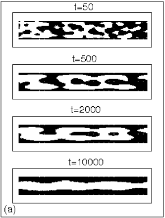
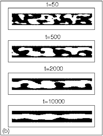
Figure 9: Cross-sectional snapshot pictures in the $xz$-plane, for $D=29,H_{\mathcal{S}1}=H_{\mathcal{S}2}=0.1$, at $k_{\rm B}T/J=5.875$ [same system as in Fig 8(a)], for four different times as indicated, according to (a) the lattice model and (b) the Ginzburg Landau model.

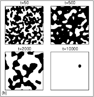
Figure 10: Same as Fig. 9, but for a plane at $n=15$, parallel to the walls.

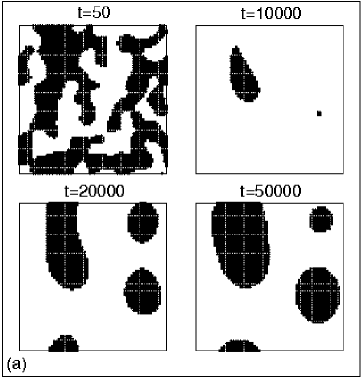
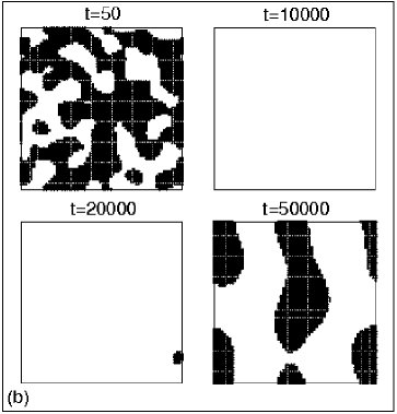
Figure 11: Same as Fig. 10, but for $D=19,~{}L=64$, at $n=10$.

In Fig. 12 we show comparisons at lower temperatures, viz., $k_{\rm B}T=5.57J$ ($\xi\simeq 1.0$, $m_{\rm b}\simeq 0.45$, $h_{\mathcal{S}1}\simeq 15.4H_{\mathcal{S}1}$, $g=-8$, $\gamma=4$, $\tau\simeq t/104$) and $k_{\rm B}T\simeq 4.75J$ ($\xi\simeq 0.5$, $m_{\rm b}\simeq 0.72$, $h_{\mathcal{S}1}\simeq 0.44H_{\mathcal{S}1}$, $g=-0.5$, $\gamma=0.5$, $\tau\simeq t/7.6$). For both the temperatures we have set $H_{\mathcal{S}1}=H_{\mathcal{S}2}=0.1$. Rather pronounced discrepancies between the lattice model and the GL model do occur, however, at low temperature [Fig. 12(b)], as expected.

Note that the prefactor $\gamma$ [see Eq. (I)] in the scaled Eq. (7) is an approximation which applies in the close vicinity of the critical point 8 . Here we try to take into account correction terms to the leading behavior of Eq. (7) to make the GL model more accurate for temperatures away from criticality. The order parameter $\phi(\vec{\rho},z,t)$ (not normalized by $m_{\rm b}$, and lengths not rescaled by 2$\xi$) satisfies the boundary conditions 8

$$2\tau_{s}\frac{\partial\phi(\vec{\rho},z=0,t)}{\partial t} = \frac{H_{1}}{T}+\frac{J}{T}\left(4\frac{J_{s}}{J}-5\right)\phi(\vec{\rho},z=0,t)~{}~{}$$ (29)

$$- \left(\frac{T_{\rm cb}}{T}-1-\frac{J}{T}\right)\frac{\partial\phi(\vec{\rho},z,t)}{\partial z}|_{z=0},$$

$$\frac{\partial}{\partial z}\{(\frac{T_{\rm cb}}{T}-1)\phi(\rho,z,t)-\frac{1}{3}[\phi(\rho,z,t)]^{3}$$

$$+\frac{J}{T}\frac{\partial^{2}}{\partial z^{2}}[\phi(\rho,z,t)]\}|_{z=0}=0.\quad$$ (30)

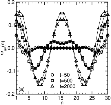
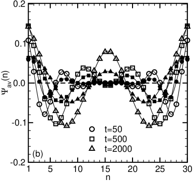
Figure 12: Plot of $\Psi_{\rm av}(n)$ vs. $n$ for $D=29$ with $H_{\mathcal{S}1}=H_{\mathcal{S}2}=0.1$ at temperatures (a) $k_{\rm B}T=5.57J$ and (b) $k_{\rm B}T=4.75J$. The open symbols corresponds to the lattice model whereas the filled symbols are for the GL model. Note that $k_{\rm B}T=5.57J$ corresponds to bulk correlation length $\xi\simeq 1.0$ and at $k_{\rm B}T=4.75J$, $\xi\simeq 0.5$.

From Eq. (29) we see, however, that a pathological behavior occurs if the coefficient $(T_{\rm cb}/T-1-J/T)$ vanishes, which is the case for $k_{\rm B}T/J=5$: the time evolution of $\phi(\vec{\rho},z=0,t)$ then is strictly decoupled from the order parameter in the interior, and it stops if $\phi(\vec{\rho},z=0,t)$ reaches the value $H_{\mathcal{S}1}/J$ (for $J_{s}/J=1)$. This is what is seen in Fig. 13(a) where we have solved the unscaled version of the GL model. In this case $\Psi_{\rm av}(z=0,t)$ has stopped its time evolution already during the very early stages. For $k_{\rm B}T<5J$ [Fig. 13(b)], the coefficient of the last term on the right side in Eq. (29) has changed its sign (in comparison to the region close to $T_{\rm cb}$), and this leads to the result that $\phi(\vec{\rho},z=0,t)$ converges to zero, which also is unreasonable. Thus, taking the coefficient $(T_{\rm cb}/T-1-J/T)$ rather than simply $(-J/T)$ [the latter leads to the scaled form Eq. (7) with the coefficient $\gamma$ as quoted in Eq. (I)] does not yield any improvement, but rather is physically inconsistent. However, working with the scaled form of the GL equations, and their boundary conditions, Eqs. (I, 5, 6, 7, 8) does not yield results in agreement with the lattice model at temperatures $k_{\rm B}T/J\leq 5$ either.

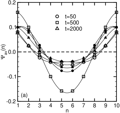
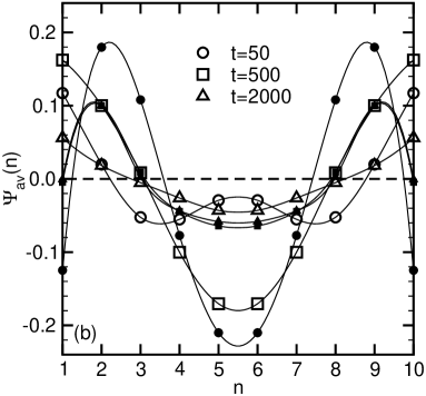
Figure 13: Comparison between the unscaled GL model [cf. Eq.(29,IV)] and lattice model at temperatures (a) $5J/k_{\rm B}$ and (b) $4J/k_{\rm B}$. Note that the open symbols are for lattice model and the filled symbols are used for the unscaled GL model.

V Conclusion

In this paper we have presented a Molecular Field Theory for the Kawasaki spin-exchange Ising model in a thin film geometry and have shown that the numerical solution of the resulting set of coupled ordinary differential equations describing the time-dependence of the local magnetization at the lattice sites is a convenient and efficient method to study spinodal decomposition of such systems, taking the boundary conditions at the surfaces of the film properly into account. Obviously, in comparison to a Monte Carlo simulation of this model one has lost thermal statistical fluctuations, except for those built into the theory via the choice of noise in the initial configuration of the system; but there is consensus 1 ; 2 ; 3 ; 4 ; 5 that for a description of the late stage coarsening behavior such thermal fluctuations may safely be neglected. Thus, the present method is favorable in comparison with Monte Carlo, since the code runs much faster.

In the vicinity of the critical point, where the correlation length $\xi$ is sufficiently large, and also the film thickness $D$ is sufficiently large as well, our treatment becomes equivalent to the time-dependent Ginzburg-Landau theory. However, one needs to go surprisingly close to the critical point of the bulk to actually demonstrate this limiting behavior from our lattice model treatment numerically. The GL treatment over most of the parameter regime provides only a qualitative, rather than quantitative, description of the system. In principle, for the GL theory to be accurate, the correlation length should be much larger than the lattice spacing. However, this happens only very close to the critical point. Away from the critical points no well-defined connection to the parameters of a microscopic Hamiltonian can be made for the GL theory, while the present lattice approach has this connection by construction.

Of course, the problem of surface-directed spinodal decomposition is most interesting for liquid binary mixtures, for which our lattice model is inappropriate due to the lack of hydrodynamic interactions; even for solid mixtures (two different atomic species sharing the sites of a lattice) our model is an idealization (neither elastic distortions nor lattice defects were included; actual solid binary mixtures decompose via the vacancy mechanism of diffusion 1 ; 2 ; etc.). While GL models including hydrodynamic interactions have been formulated 1 ; 2 ; 3 ; 4 ; 5 , the restriction that any GL model is valid only in the immediate neighborhood of the critical point applies there as well. While outside the critical region unmixing of fluids can be simulated by Molecular Dynamics methods (see e.g. 19 ), such simulations are extremely time-consuming, and an analog of the present dynamic mean field theory for inhomogeneous fluids would be very desirable. Developing such an approach clearly is a challenge for the future.

Acknowledgments: This work was supported in part by the Deutsche Forschungsgemeinschaft (DFG), grant number SFB-TR6/A5. K.B. is very much indebted to Prof. S. Puri and the late Prof. H.L. Frisch for stimulating his interest in these problems and for many discussions. S.K.D. is grateful to K.B. for supporting his stay in Mainz, where this work was initiated and acknowledges useful discussions with Prof. S. Puri.

References

- (1) K. Binder and P. Fratzl, in Phase Transformations in Materials, edited by G. Kostorz (Wiley-VCH, Weinheim, 2001) p. 409.
- (2) A. Onuki, Phase Transition Dynamics (Cambridge University Press, Cambridge, 2002).
- (3) J.D. Gunton, M. San Miguel, and P.S. Sahni, in Phase Transitions and Critical Phenomena, edited by C. Domb and J.L. Lebowitz (Academic Press, London, 1983), Vol. 8, p. 267.
- (4) A.J. Bray, Adv. Phys. 43, 357 (1994).
- (5) S. Dattagupta and S. Puri, Dissipative Phenomena in Condensed Matter: Some Applications (Springer, Berlin, 2004).
- (6) Dynamics of Ordering Processes in Condensed Matter, edited by S. Komura and H. Furukawa (Plenum Press, New York, 1988).
- (7) R.A.L. Jones, L.J. Norton, E.J. Kramer, F.S. Bates and P. Wiltzius, Phys. Rev. Lett. 66, 1326 (1991).
- (8) S. Puri and K. Binder, Phys. Rev. A46, R4487 (1992); Phys. Rev. E49, 5359 (1994).
- (9) G. Brown and A. Chakrabarti, Phys. Rev. A46, 4829 (1992).
- (10) S. Puri and K. Binder, J. Stat. Phys. 77, 145 (1994).
- (11) G. Krausch, Mater. Sci. Eng. R14, 1 (1995).
- (12) S. Puri and H.L. Frisch, J. Phys.: Condens. Matter 9, 2109 (1997).
- (13) K. Binder, J. Non-Nquilib. Thermodyn. 23, 1 (1998).
- (14) S. Puri and K. Binder, Phys. Rev. Lett. 86, 1797 (2001); Phys. Rev. E66, 061602 (2002).
- (15) S. Bastea, S. Puri, and J.L. Lebowitz, Phys. Rev. E63, 041513 (2001).
- (16) J.M. Geoghegan and G. Krausch, Prog. Polym. Sci. 28, 261 (2003).
- (17) S. Puri, J. Phys.: Condens. Matter 17, R101 (2005).
- (18) S.K. Das, S. Puri, J. Horbach, and K. Binder, Phys. Rev. E72, 061603 (2005).
- (19) S.K. Das, S. Puri, J. Horbach, and K. Binder, Phys. Rev. Lett. 96, 016107 (2006); Phys. Rev. E73, 031604 (2006).
- (20) K. Binder and H.L. Frisch, Z. Physik B: Condens. Matter 84, 403 (1991).
- (21) K. Binder, in Phase Transitions and Critical Phenomena, edited by C. Domb and J.L. Lebowitz (Academic Press, London, 1983) Vol. 8, p.1.
- (22) H.W. Diehl, in Phase Transitions and Critical Phenomena, edited by C. Domb and J.L. Lebowitz (Academic Press, London, 1986), Vol, 10, p. 75.
- (23) J.W. Cahn, J. Chem. Phys. 66, 3667 (1977).
- (24) M.E. Fisher, J. Stat. Phys. 34, 667 (1984); J. Chem. Soc., Faraday Trans. II, 82, 1569 (1986).
- (25) P.G. de Gennes, Rev. Mod. Phys. 57, 827 (1985).
- (26) D.E. Sullivan and M.M. Telo da Gama, in Fluid Interfacial Phenomena, edited by C.A. Croxton (Wiley, New York, 1986) p. 45.
- (27) S. Dietrich, in Phase Transitions and Critical Phenomena, edited by C. Domb and J.L. Lebowitz (Academic Press, London, 1988) Vol 12, p. 1.
- (28) M. Schick, in Liquids at Interfaces, edited by J. Charvolin, J.-F. Joanny and J. Zinn-Justin (North-Holland, Amsterdam, 1990) p. 415.
- (29) K. Binder, D.P. Landau, and M. Müller, J. Stat. Phys. 110, 1411 (2003).
- (30) D.M. Kroll and G. Gompper, Phys. Rev. B39, 433 (1989).
- (31) K. Binder and D.P. Landau, J. Chem. Phys. 96, 1444 (1992).
- (32) M.E. Fisher and H. Nakanishi, J. Chem. Phys. 75, 5857 (1981).
- (33) R. Evans, J. Phys.: Condens. Matter 2, 8989 (1990).
- (34) L.D. Gelb, K.E. Gubbins, R. Radhakrishnan, and M. Sliwinska-Bartkowiak, Rep. Prog. Phys. 62, 1573 (1999).
- (35) M. Müller, K. Binder, and E.V. Albano, Physica A279, 188 (2000); Int. J. Mod. Phys. B15, 1867 (2001).
- (36) M. Müller, K. Binder, and E.V. Albano, Europhys. Lett. 50, 724 (2000).
- (37) M. Müller and K. Binder, J. Phys.: Condens. Matter 17, S333 (2005).
- (38) P.C. Hohenberg and B.I. Halperin, Rev. Mod. Phys. 49, 435 (1977).
- (39) I. Schmidt and K. Binder, Z. Phys. B: Condens. Matter 67, 369 (1987).
- (40) K. Binder, Z. Phys. 267, 313 (1974).
- (41) K. Kawasaki, in Phase Transitions and Critical Phenomena, edited by C. Domb and M.S. Green (Academic Press, London, 1972) Vol 2, Chapter 11.
- (42) R.J. Glauber, J. Math. Phys. 4, 294 (1963).
- (43) I.M. Lifshitz and V.V. Slyozov, J. Phys. Chem. Solids 19, 35 (1961).
- (44) J.G. Amar, F.E. Sullivan, and R.D. Mountain, Phys. Rev. B 37, 196 (1988).