Imperial/TP/2008/JG/03

DESY 08-147

$AdS_{3}\times_{w}(S^{3}\times S^{3}\times S^{1})$ Solutions
of Type IIB String Theory
Aristomenis Donos¹, Jerome P. Gauntlett² and James Sparks³

¹DESY Theory Group, DESY Hamburg
Notkestrasse 85, D 22603 Hamburg, Germany
²Theoretical Physics Group, Blackett Laboratory,
Imperial College, London SW7 2AZ, U.K.
²The Institute for Mathematical Sciences,
Imperial College, London SW7 2PE, U.K.
³Mathematical Institute, University of Oxford,
24-29 St Giles’, Oxford OX1 3LB, U.K.

Abstract

We analyse a recently constructed class of local solutions of type IIB supergravity that consist of a warped product of $AdS_{3}$ with a seven-dimensional internal space. In one duality frame the only other non-vanishing fields are the NS three-form and the dilaton. We analyse in detail how these local solutions can be extended to give infinite families of globally well-defined solutions of type IIB string theory, with the internal space having topology $S^{3}\times S^{3}\times S^{1}$ and with properly quantised three-form flux.

1 Introduction

Supersymmetric solutions of string or M-theory that contain $AdS_{d+1}$ factors are dual to supersymmetric conformal field theories in $d$ spacetime dimensions. Starting with the work of [1], general characterisations of the geometries underlying such solutions, using $G$-structure techniques [2, 3], have been achieved for various $d$ and for various amounts of supersymmetry [4]–[23]. With a few exceptions, mostly with sixteen supersymmetries, many of these geometries are still poorly understood, and it has proved difficult to find explicit solutions.

One notable exception is the class of $AdS_{3}$ solutions of type IIB string theory with non-vanishing five-form flux, dual to $d=2$ conformal field theories with $(0,2)$ supersymmetry, that were classified in [7]. It was shown that the seven-dimensional internal space has a Killing vector which is dual to the $R$-symmetry of the dual SCFT. The Killing vector defines a foliation and the solution is completely determined, locally, by a Kähler metric on the six-dimensional leaf space whose Ricci tensor satisfies an additional differential condition. Moreover, a rich set of explicit solutions have been constructed in [24, 14, 25] and the corresponding central charges of the dual SCFTs have also been calculated.

More recently, it was understood how to generalise this class of type IIB $AdS_{3}$ solutions to also include three-form flux [26]. The solutions are again locally determined by a six-dimensional Kähler metric and a choice of a closed, primitive $(1,2)$-form on the Kähler space. Once again additional explicit solutions were constructed with the six-dimensional Kähler space having a two-torus factor and the three-form flux being parametrised by a real parameter $Q$. After two T-dualities on the two-torus it was also shown that these explicit solutions give type IIB $AdS_{3}$ solutions with non-vanishing dilaton and RR three-form flux only. After an additional $S$-duality the solutions only involve NS fields.

In [26] these explicit solutions were examined in more detail for the special case of $Q=0$. It was shown that the parameters and ranges of the coordinates could be chosen to give globally defined supergravity solutions consisting of a warped product of $AdS_{3}$ with a seven-dimensional internal manifold that is diffeomorphic to $S^{2}\times S^{3}\times T^{2}$. It was shown that the solutions, with properly quantised three-form flux, are specified by a pair of positive coprime integers $p,q$.

The purpose of this paper is to carry out a similar analysis when we switch on the parameter $Q$. We will find that we are led to infinite classes of solutions, with the seven-dimensional internal space being diffeomorphic to $S^{3}\times S^{3}\times S^{1}$ and with properly quantised fluxes.

While the final topology of the solutions is simple, it is not easy to see this in the local coordinates in which the solutions are presented. When $Q=0$ the $S^{2}\times S^{3}$ factor is realised in a manner very similar to the $Y^{p,q}$ Sasaki-Einstein spaces [27]. When $Q\neq 0$ one of the circles in the $T^{2}$ factor is fibred over the $S^{2}\times S^{3}$ and we need to carefully check that the circle fibration is globally well-defined, leading to $S^{3}\times S^{3}$. Furthermore we need to check that the three-form flux is properly quantised. This is not straightforward since it is not clear “where” the two $S^{3}$ factors are in the local coordinates. After some false starts we developed a workable prescription for ensuring that the three-form is properly quantised, as we shall explain.

The plan of the paper is as follows. In section 2, we begin by recalling the local solutions of [26] and then discuss how, after suitable choices of parameters and periods for the coordinates, the seven-dimensional internal manifold has topology $S^{3}\times S^{3}\times S^{1}$. We discuss some aspects of the topology in detail, leading to a prescription for carrying out flux quantisation which is dealt with in section 3. Our method uses a quotient construction, which is explained in section 2, as well as explicit coordinate patches. In sections 2 and 3, the solutions depend on a pair of coprime positive integers $p,q$, the electric three-form flux, $n_{1}$, the magnetic three-form flux through each of the two $S^{3}$ factors, $M_{1}$ and $M_{2}$, and the parameter $Q$. For these solutions, it turns out that $M_{1}$ and $M_{2}$ are not independent and are given by $M_{1}=M(p+q)^{2}$ and $M_{2}=Mq^{2}$, where $M$ is an integer. We calculate the central charge and show that it is given by the simple formula

$$c=6n_{1}\frac{(M_{1}-M_{2})M_{2}}{M_{1}}~{}.$$ (1.1)

In particular it is independent of $Q$, and since the solutions with $Q\neq 0$ and other parameters fixed are all smoothly connected with each other, we conclude that when $Q\neq 0$, the parameter $Q$ corresponds to an exactly marginal deformation in the dual $(0,2)$ SCFT. It is interesting to observe that the value of the central charge is precisely the same as for the $Q=0$ solutions studied in [26]. However, as we shall explain in section 3.3 taking the limit $Q\to 0$ does not smoothly lead to the $Q=0$ solutions and so it is not clear whether or not the $Q\neq 0$ solutions correspond to exactly marginal deformations of the $Q=0$ solutions.

In section 4, we generalise our construction by making more general identifications on the coordinates, obtaining solutions that involve more parameters. We show that the central charge has exactly the same form as in (1.1), but now, however, the integers $M_{1}$ and $M_{2}$ labelling the three-form flux through the two $S^{3}$’s are no longer constrained. Thus not all of these more general solutions correspond to exactly marginal deformations of those that we consider in sections 2 and 3. We conclude in section 5.

We noted above that the $S^{2}\times S^{3}$ factor in the $AdS_{3}$ solutions constructed in [26], with $Q=0$, is realised in a similar way to the $Y^{p,q}$ Sasaki-Einstein spaces found in [27]. In particular, in both cases the metrics on $S^{2}\times S^{3}$ are cohomogeneity one. Given that the $Y^{p,q}$ metrics can be generalised to cohomogeneity two Sasaki-Einstein metrics $L^{a,b,c}$ on $S^{2}\times S^{3}$ [28] (see also [29]), it is natural to suspect that there are analogous $AdS_{3}$ solutions, with five-form flux only, with internal space having topology $S^{2}\times S^{3}\times T^{2}$ and with the metric on the $S^{2}\times S^{3}$ factor having cohomogeneity two. This is indeed possible, and moreover it is also possible to find generalisations with non-zero three-form flux and with the internal manifold having topology $S^{3}\times S^{3}\times S^{1}$. We will present such solutions in appendix C, but we will leave a detailed analysis of the regularity and flux quantisation conditions for future work.

2 The $AdS_{3}$ solutions

2.1 The local solutions

We start with the explicit class of $AdS_{3}$ solutions of section 4.3 of [26]. The string frame metric is given by

$$\frac{1}{L^{2}}ds^{2}=\frac{\beta}{y^{1/2}}[ds^{2}(AdS_{3})+ds^{2}(X_{7})]$$ (2.1)

where

$$ds^{2}(X_{7}) = \frac{\beta^{2}-1+2y-Q^{2}y^{2}}{4\beta^{2}}Dz^{2}+\frac{U(y)}{4(\beta^{2}-1+2y-Q^{2}y^{2})}D\psi^{2}+\frac{dy^{2}}{4\beta^{2}y^{2}U(y)}$$ (2.2)

$$+\frac{1}{4\beta^{2}}ds^{2}(S^{2})+(du^{1}-\frac{Qy}{2\beta}[(1-g)D\psi-Dz])^{2}+(du^{2})^{2}\ ~{},$$

where $\beta,Q$ are positive constants, $L$ is an arbitrary length scale and

$$U(y)=1-\frac{1}{\beta^{2}}(1-y)^{2}-Q^{2}y^{2}~{}.$$ (2.3)

In addition, $ds^{2}(S^{2})$ is the standard metric on a two-sphere, $ds^{2}(S^{2})=d\theta^{2}+\sin^{2}\theta d\phi^{2}$, and we have defined

$$D\psi=d\psi+P$$ (2.4)

with

$$dP=\mathrm{Vol}(S^{2})=\sin\theta d\theta\wedge d\phi\equiv J~{}.$$ (2.5)

Note that $P$ is only a locally defined one-form on $S^{2}$. In fact, more precisely, $P$ is a connection one-form on the $U(1)$ principal bundle associated to the tangent bundle of $S^{2}$. The two-form $J$ introduced in (2.5) may be regarded as a Kähler form on $S^{2}$. We also have

$$Dz=dz-g(y)D\psi$$ (2.6)

with

$$g(y)=\frac{y(1-Q^{2}y)}{\beta^{2}-1+2y-Q^{2}y^{2}}~{}.$$ (2.7)

The only other non-trivial type IIB supergravity fields are the dilaton and the RR three-form. The dilaton is given by

$$e^{2\phi}=\frac{\beta^{2}}{y}$$ (2.8)

while the RR three-form field strength is given by

$$\frac{1}{L^{2}}F^{(3)} = -\frac{1}{4\beta^{2}}dy\wedge D\psi\wedge Dz-\frac{y}{4\beta^{2}}J\wedge Dz+\left[\frac{1-yg}{4\beta^{2}}\right]J\wedge D\psi$$ (2.9)

$$+\frac{Q}{2\beta}du^{1}\wedge[dy\wedge Dz-yJ-(1-g)dy\wedge D\psi]+2\mathrm{Vol}(AdS_{3})~{}.$$

This is closed. After a further $S$-duality transformation we obtain $AdS_{3}$ solutions with only NS fields non-vanishing, but we will continue to work with the above solution.

In order to simplify some of the formulae it will be helpful to introduce

$$Z\equiv 1-\sqrt{1+Q^{2}(\beta^{2}-1)}~{}.$$ (2.10)

We next change coordinates via

$$dz = dw+\frac{2Q\beta}{Z-2}\,dv$$

$$du^{1} = dv+\,\frac{Q(1-\beta^{2})}{2\beta(Z-2)}dw$$ (2.11)

to bring the metric to the form

$$ds^{2}(X_{7})=\frac{2(1-Z)(1-\beta^{2}-yZ)}{(2-Z)(1-\beta^{2})}Dv^{2}+\frac{(1-Z)(2y-yZ-1+\beta^{2})}{2\beta^{2}(2-Z)}Dw^{2}$$

$$+\frac{(1-\beta^{2})U(y)}{4(1-\beta^{2}-Zy)(\beta^{2}-1+2y-Zy)}D\psi^{2}+\frac{dy^{2}}{4\beta^{2}y^{2}U(y)}+\frac{1}{4\beta^{2}}ds^{2}(S^{2})+(du^{2})^{2}$$

where

$$Dv = dv-A_{v}\,D\psi$$

$$Dw = dw-A_{w}\,D\psi$$ (2.13)

and

$$A_{v} = \frac{Q(1-\beta^{2})y}{4\beta(1-\beta^{2}-yZ)}$$

$$A_{w} = \frac{(2-Z)y}{2(2y-yZ-1+\beta^{2})}~{}.$$ (2.14)

The three-form in the new coordinates is given by

$$\frac{1}{{L}^{2}}F^{(3)} = 2\,\mathrm{Vol}\left(AdS_{3}\right)+\frac{(1-\beta^{2})U(y)}{4(1-\beta^{2}-yZ)(\beta^{2}-1+2y-yZ)}\,J\wedge D\psi$$

$$- Dw\wedge\left\{\frac{(Z-1)(1-\beta^{2})}{4\beta^{2}(Zy-1+\beta^{2})}dy\wedge D\psi+\frac{y(1-Z)}{4\beta^{2}}J\right\}$$

$$- QDv\wedge\left\{\frac{(1-Z)(1-\beta^{2})}{2\beta(Z-2)(-Zy-1+\beta^{2}+2y)}dy\wedge D\psi+\frac{y(1-Z)}{2\beta(2-Z)}J\right\}$$

$$- \frac{Q(1-Z)}{\beta(2-Z)}dy\wedge Dv\wedge Dw~{}.$$

Finally, we note that the canonical Killing vector related to supersymmetry is given by

$$\partial_{\psi}+\partial_{z}~{}.$$ (2.16)

In the new coordinates this reads

$$\partial_{\psi}+\frac{(Z-2)}{2(Z-1)}\partial_{w}+\frac{Q(\beta^{2}-1)}{4\beta(Z-1)}\partial_{v}~{}.$$ (2.17)

We now would like to find the restrictions on the parameters $\beta$, $Q$ so that these local solutions extend to global solutions on a globally well-defined manifold $X_{7}$. Having achieved that goal, we will analyse the additional constraints imposed by ensuring that the three-form is properly quantised. Note that when $Q=0$ the corresponding analysis was carried out in [26] and in particular it was shown that there were infinite classes of solutions, labelled by a pair of positive coprime integers, $p,q$, with $X_{7}$ having the topology of $S^{3}\times S^{2}\times T^{2}$.

Our strategy is to build $X_{7}$ in stages. The $u^{2}$ coordinate is taken to paramaterise an $S^{1}$: for now the period of $u^{2}$ is arbitrary but it will later be fixed by flux quantisation. We therefore write $X_{7}=M_{6}\times S^{1}$ with

$$ds^{2}(M_{6})\equiv\frac{2(1-Z)(1-\beta^{2}-yZ)}{(2-Z)(1-\beta^{2})}Dv^{2}+ds^{2}(M_{5})\ ,$$ (2.18)

where

$$ds^{2}(M_{5})\equiv\frac{(1-Z)(2y-yZ-1+\beta^{2})}{2\beta^{2}(2-Z)}Dw^{2}+ds^{2}(B_{4})$$ (2.19)

and

$$ds^{2}(B_{4})\equiv\frac{(1-\beta^{2})U(y)}{4(1-\beta^{2}-Zy)(\beta^{2}-1+2y-Zy)}D\psi^{2}+\frac{dy^{2}}{4\beta^{2}y^{2}U(y)}+\frac{1}{4\beta^{2}}ds^{2}(S^{2})~{}.$$ (2.20)

We will first analyse $ds^{2}(B_{4})$, showing that, by taking $\psi$ to be a periodic coordinate with period $2\pi$, $B_{4}$ is a smooth manifold diffeomorphic to $S^{2}\times S^{2}$. We then show that, by taking $w$ to be a periodic coordinate with a suitable period, with the parameter $\beta$ fixed by two relatively prime positive integers $p,q$, $M_{5}$ is the total space of a circle fibration over $B_{4}$, and has topology $S^{3}\times S^{2}$. Here $p$ and $q$ have a topological interpretation as Chern numbers of the circle bundle over $B_{4}$. These steps are familiar from the construction of the Sasaki-Einstein manifolds $Y^{p,q}$ [27] (and also for the $Q=0$ solutions studied in [26]). The final step is to show that, by taking $v$ to be periodic with a suitable period, $M_{6}$ is the total space of a circle fibration over $M_{5}$, and has topology $S^{3}\times S^{3}$.

It will be useful in the following to observe that the function $U(y)$ is a quadratic function of $y$ with roots $y_{1}$ and $y_{2}$ given by

$$y_{1} = \frac{1-\beta^{2}}{1+\beta(1-Z)}$$

$$y_{2} = \frac{1-\beta^{2}}{1-\beta(1-Z)}~{}.$$ (2.21)

It will also be useful to know the values of the functions $A_{w}$ and $A_{v}$ appearing in $ds^{2}(M_{6})$ at $y_{1}$ and $y_{2}$. We find

$$A_{w}(y_{1}) = \frac{2-Z}{2(1-Z)(1-\beta)}$$

$$A_{w}(y_{2}) = \frac{2-Z}{2(1-Z)(1+\beta)}$$

$$A_{v}(y_{1}) = \frac{Q(1-\beta)}{4\beta(1-Z)}$$

$$A_{v}(y_{2}) = \frac{Q(1+\beta)}{4\beta(1-Z)}~{}.$$ (2.22)

2.2 $B_{4}=S^{2}\times S^{2}$

$B_{4}$ is parametrised by $\theta$, $\phi$, $y$ and $\psi$. We take the coordinate $y$ to lie in the interval $y\in[y_{1},y_{2}]$ where $y_{i}$ are the two distinct positive roots of $U(y)$, given by (2.1). This requires that we demand

$$0<\beta<1,\qquad 0\leq Z<1~{}.$$ (2.23)

We next observe that if we choose the period of $\psi$ to be $2\pi$, then $y,\psi$ parametrise a smooth two-sphere, with $y$ a polar coordinate and $\psi$ an azimuthal coordinate on the metrically squashed $S^{2}$ fibre. In particular, fixing a point on the round two-sphere, one can check that $ds^{2}(B_{4})$ is free from conical singularities at the poles $y=y_{1}$ and $y=y_{2}$. $B_{4}$ is then a smooth $S^{2}$ bundle over the round $S^{2}$. The transition functions are in $U(1)$, acting in the obvious way on the fibre. The first Chern number of the $U(1)$ fibration is $-2$ and thus, as explained in [27], $B_{4}$ is diffeomorphic to $S^{2}\times S^{2}$.

We have $H_{2}(B_{4},{\mathbb{Z}})\cong{\mathbb{Z}}\oplus{\mathbb{Z}}$. Three obvious two-spheres in $B_{4}$ are the sections $\Sigma_{1}=\{y=y_{1}\}$ and $\Sigma_{2}=\{y=y_{2}\}$, each a copy of the two-sphere base, and a copy of the fibre $\Sigma_{f}$ at some point on the two-sphere base (for concreteness, say, the north pole $\{\theta=0\}$). Call the corresponding homology classes $[\Sigma_{1}]$, $[\Sigma_{2}]$ and $[\Sigma_{f}]$, respectively. We can take $[\Sigma_{2}]$ and $[\Sigma_{f}]$ to generate $H_{2}(B_{4},{\mathbb{Z}})$, but we note that this is not the natural basis of $S^{2}\times S^{2}$. In particular, the intersections of the 2-cycles are

$$[\Sigma_{f}]\cap[\Sigma_{f}]=0,\quad[\Sigma_{f}]\cap[\Sigma_{2}]=1,\quad[\Sigma_{2}]\cap[\Sigma_{2}]=2~{}.$$ (2.24)

The only non-obvious equality above is the last. This follows since the self-intersection of a 2-cycle in a 4-manifold is equal to the Chern number of the normal bundle. Similar calculations show that

$$[\Sigma_{1}]=[\Sigma_{2}]-2[\Sigma_{f}].$$ (2.25)

Later it will be useful to use a more natural basis given by $[C_{1}]=[\Sigma_{2}]-[\Sigma_{f}]$ and $[C_{2}]=[\Sigma_{f}]$: indeed one can then check that $[C_{1}]\cap[C_{1}]=[C_{2}]\cap[C_{2}]=0$ and $[C_{1}]\cap[C_{2}]=1$.

By Poincaré duality we have $H_{2}(B_{4},{\mathbb{Z}})\cong H^{2}(B_{4},{\mathbb{Z}})$. Recall that, by definition, the Poincare dual $\eta_{\Sigma}$ of a submanifold $\Sigma\subset M$ satisfies

$$\int_{\Sigma}\omega=\int_{M}\omega\wedge\eta_{\Sigma}$$ (2.26)

for any closed form $\omega$. We introduce the closed two-forms on $B_{4}$

$$\sigma_{2} = \frac{1}{4\pi}J$$

$$\sigma_{f} = \frac{1}{2\pi[A_{w}(y_{1})-A_{w}(y_{2})]}[(A_{w}(y_{2})-A_{w})J-\partial_{y}(A_{w})dy\wedge D\psi]~{}.$$ (2.27)

These forms satisfy

$$\int_{\Sigma_{2}}\sigma_{2}=\int_{\Sigma_{f}}\sigma_{f}=1,\qquad\int_{\Sigma_{2}}\sigma_{f}=\int_{\Sigma_{f}}\sigma_{2}=0~{},$$ (2.28)

and one finds that Poincaré duality maps $\Sigma_{f}\mapsto\sigma_{2}$ and $\Sigma_{2}\mapsto\sigma_{f}+2\sigma_{2}$.

2.3 $M_{5}=S^{3}\times S^{2}$

We next construct $M_{5}$ as the total space of a circle bundle over $B_{4}$, by letting $w$ be periodic with period $2\pi l_{w}$, for a suitably chosen $l_{w}$. We begin by observing from (2.1) that the norm of the Killing vector $\partial_{w}$ is nowhere-vanishing, and so the size of the $S^{1}$ fibre doesn’t degenerate anywhere. Recalling that $Dw=dw-A_{w}\,D\psi$, we require that $l_{w}^{-1}A_{w}D\psi$ is a connection on a bona fide $U(1)$ fibration with first Chern class represented by $(2\pi l_{w})^{-1}d(A_{w}\,D\psi)$.

It is straightforward to first check that $(2\pi l_{w})^{-1}d(A_{w}\,D\psi)$ is indeed a globally defined two-form on $B_{4}$. We next impose that it has integer valued periods:

$$\frac{1}{2\pi l_{w}}\int_{\Sigma_{2}}d\left(A_{w}D\psi\right) = \frac{2}{l_{w}}A_{w}\left(y_{2}\right)=p$$

$$\frac{1}{2\pi l_{w}}\int_{\Sigma_{f}}d\left(A_{w}D\psi\right) = \frac{1}{l_{w}}\left[A_{w}\left(y_{2}\right)-A_{w}\left(y_{1}\right)\right]=-q,$$ (2.29)

where $p,q$ are positive integers. One can then calculate

$$\frac{1}{2\pi l_{w}}\int_{\Sigma_{1}}d\left(A_{w}D\psi\right)=\frac{2}{l_{w}}A_{w}\left(y_{1}\right)=p+2q$$ (2.30)

as expected from (2.25). We then deduce that

$$\beta=\frac{q}{p+q}$$ (2.31)

which, remarkably, is independent of $Q$, and

$$l_{w}=\frac{2-Z}{p(1-Z)(1+\beta)}~{}.$$ (2.32)

With these choices we have that $M_{5}$ is the total space of a circle bundle with first Chern class given by

$$c_{1}=p[\sigma_{2}]-q[\sigma_{f}]\in H^{2}(B_{4},{\mathbb{Z}})~{}.$$ (2.33)

As in [27], taking $p$ and $q$ to be relatively prime, as we shall henceforth do, one can show that $M_{5}$ is simply-connected with $H_{2}(M_{5},{\mathbb{Z}})\cong{\mathbb{Z}}$. Using Smale’s theorem for five-manifolds [30], it follows that $M_{5}$ is diffeomorphic to $S^{3}\times S^{2}$.

Having constructed $M_{5}$, it will be useful later to know various topological properties of this manifold in terms of the coordinate system above. In the remainder of this subsection we write down explicit generators for $H^{2}(M_{5},{\mathbb{Z}})\cong{\mathbb{Z}}$, which will be useful for constructing circle bundles over $M_{5}$, and for $H^{3}(M_{5},{\mathbb{Z}})\cong{\mathbb{Z}}$, which will be useful both for integration using Poincaré duality and also for quantising the three-form flux. We also find representatives of the generating 2-cycle and 3-cycle in $H_{2}(M_{5},{\mathbb{Z}})\cong{\mathbb{Z}}$ and $H_{3}(M_{5},{\mathbb{Z}})\cong{\mathbb{Z}}$, respectively.

The generator of $H^{2}(M_{5},{\mathbb{Z}})\cong{\mathbb{Z}}$ may be taken to be the pull-back of the class

$$\tau=b[\sigma_{2}]+a[\sigma_{f}]\in H^{2}(B_{4},{\mathbb{Z}})$$ (2.34)

under the projection

$$\pi:M_{5}\rightarrow B_{4}~{},$$ (2.35)

where $a$ and $b$ are (any) integers satisfying

$$pa+qb=1~{}.$$ (2.36)

These exist and are unique up to $b\rightarrow b+mp$, $a\rightarrow a-mq$, for any integer $m$, by Bezout’s lemma. The non-uniqueness simply corresponds to the fact that the Chern class $c_{1}=p\sigma_{2}-q\sigma_{f}$ of the circle bundle over $B_{4}$ is trivial when pulled back to $M_{5}$, as is the Chern class of any tensor power of this circle bundle (the power corresponds to the integer $m$ above).

To see that $\pi^{*}\tau$ is the generator of $H^{2}(M_{5},{\mathbb{Z}})$ as claimed, note that, a priori, $\pi^{*}\tau$ is necessarily $\delta$ times the generator, for some integer $\delta\in{\mathbb{Z}}$. Thus we write $\pi^{*}\tau=\delta\in H^{2}(M_{5},{\mathbb{Z}})\cong{\mathbb{Z}}$. Next note that the circle bundle $\pi$ trivialises over any smooth submanifold $S\subset B_{4}$ that represents the cycle

$$[S]=q[\Sigma_{2}]+p[\Sigma_{f}]~{}.$$ (2.37)

This is simply because the first Chern class $c_{1}$ evaluated on $[S]$ is zero, as one sees using (2.28). Hence we may take a section $s$ of $\pi$ over $S$:

$$s:S\rightarrow M_{5}~{}.$$ (2.38)

This defines a 2-cycle $[s(S)]$ in $H_{2}(M_{5},{\mathbb{Z}})\cong{\mathbb{Z}}$, which we may take to be $\alpha$ times the generator, for some integer $\alpha$. But then by construction

$$\int_{s(S)}\pi^{*}\tau=\int_{S}\tau=1~{},$$ (2.39)

implying that $\alpha\delta=1$, and thus $\alpha$ and $\delta$ are both $\pm 1$. Hence $\pi^{*}\tau$ generates $H^{2}(M_{5},{\mathbb{Z}})$, and $s(S)$ generates $H_{2}(M_{5},{\mathbb{Z}})$.

The only other non-trivial homology group is $H_{3}(M_{5},{\mathbb{Z}})\cong{\mathbb{Z}}$. There are three natural three-submanifolds of $M_{5}$, which we call $E_{1}$, $E_{2}$ and $E_{f}$. These are the restriction of the circle bundle $\pi$ to the submanifolds $\Sigma_{1}$, $\Sigma_{2}$ and $\Sigma_{f}$ of $B_{4}$, respectively. These three-manifolds are all Lens spaces. Indeed, $\Sigma_{1}$, $\Sigma_{2}$, $\Sigma_{f}$ are all two-spheres. The Chern numbers are easily read off from $c_{1}$ above to be $p+2q$, $p$ and $-q$. Thus

$$E_{1}\cong S^{3}/{\mathbb{Z}}_{p+2q},\quad E_{2}\cong S^{3}/{\mathbb{Z}}_{p},\quad E_{f}\cong S^{3}/{\mathbb{Z}}_{q}~{}.$$ (2.40)

We may take the generator of $H_{3}(M_{5},{\mathbb{Z}})$ to be

$$E=k[E_{1}]+l[E_{f}]$$ (2.41)

where $k$ and $l$ are (any) integers satisfying

$$pk+ql=1~{}.$$ (2.42)

Notice this is the same as (2.36), so one could choose $k=a$ and $l=b$. A simple way to check this is to note that the generator has intersection number 1 with $[s(S)]$. One computes

$$[s(S)]\cap E=pk+ql=1$$ (2.43)

which uniquely identifies $E$ as the generator. We then have

$$[E_{1}]=pE,\qquad[E_{2}]=(p+2q)E,\qquad[E_{f}]=qE~{},$$ (2.44)

which again can be shown by taking intersection numbers with $[s(S)]$.

Finally, we may also write down a representative $\Phi$ of the generator of $H^{3}(M_{5},\mathbb{Z})$. By definition this is a closed three-form on $M_{5}$ that integrates to 1 over $E$. We choose

$$\Phi=\frac{1}{\left(2\pi\right)^{2}l_{w}^{2}} \left\{Dw\wedge\left[\left(A_{w}\left(y_{1}\right)+A_{w}\left(y_{2}\right)-A_{w}\left(y\right)\right)J-\partial_{y}A_{w}dy\wedge D\psi\right]\right.$$

$$\left.-\left[A_{w}^{2}(y)-A_{w}\left(y\right)\left(A_{w}\left(y_{1}\right)+A_{w}\left(y_{2}\right)\right)+A_{w}\left(y_{1}\right)A_{w}\left(y_{2}\right)\right]\,J\wedge D\psi\right\}.$$ (2.45)

The three-form $\Phi$ is Poincaré dual to the non-trivial two-cycle in $M_{5}$.

2.4 $M_{6}=S^{3}\times S^{3}$

We now construct $M_{6}$ as a circle bundle over $M_{5}$. Since $H^{2}(M_{5},{\mathbb{Z}})\cong{\mathbb{Z}}$, such circle bundles are determined, up to isomorphism, by an integer. Since $M_{5}\cong S^{3}\times S^{2}$, taking this integer to be $1$ (or $-1$) gives a total space $M_{6}\cong S^{3}\times S^{3}$. Taking the Chern number to be $n$ would instead lead to an $M_{6}$ with $\pi_{1}(M_{6})\cong{\mathbb{Z}}_{n}$, which we may always lift to the simply-connected cover with $n=\pm 1$. So, we will do this. However, as we shall see later, in fixing the three-form flux quantisation it will be helpful to consider such quotients of $M_{6}$.

Observe from (2.1) that the norm of the Killing vector $\partial_{v}$ is nowhere-vanishing, and so the size of the $S^{1}$ fibre doesn’t degenerate anywhere. The period of $v$ is taken to be $2\pi l_{v}$, where $l_{v}$ will be fixed shortly. Recalling that $Dv=dv-A_{v}\,D\psi$, we require that $l_{v}^{-1}A_{v}D\psi$ is a connection on a $U(1)$ fibration with first Chern class represented by $(2\pi l_{v})^{-1}d(A_{v}\,D\psi)$. It is straightforward to check that $(2\pi l_{v})^{-1}d(A_{v}\,D\psi)$ is a globally defined two-form on $M_{5}$. We next impose that it has unit period. To do this we would like to integrate $(2\pi l_{v})^{-1}d(A_{v}\,D\psi)$ over a smooth submanifold in the same homology class as $s(S)$, the generator of $H_{2}(M_{5},{\mathbb{Z}})$. However, as we have already noted, finding such a smooth submanifold is not so easy. Luckily, we can use Poincaré duality to calculate the period instead. Recalling that $[\Phi]$ is Poincaré dual to $[s(S)]$, we demand that

$$\frac{1}{2\pi l_{v}}\int_{s(S)}d(A_{v}D\psi) = \frac{1}{2\pi l_{v}}\int_{M_{5}}d(A_{v}D\psi)\wedge\Phi$$ (2.46)

$$= \frac{2}{l_{v}l_{w}}[A_{v}(y_{2})A_{w}(y_{1})-A_{v}(y_{1})A_{w}(y_{2})]$$

$$= \frac{1}{l_{v}}[2qA_{v}(y_{2})-p(A_{v}(y_{1})-A_{v}(y_{2}))]=1,$$

so that the circle bundle has Chern number 1, which can be achieved by setting

$$l_{v}=\frac{Q(p+q)}{1-Z}~{}.$$ (2.47)

Let us denote this circle bundle over $M_{5}$ by $L$, with corresponding projection

$$\Pi:M_{6}\to M_{5}~{}.$$ (2.48)

Recalling that the generator of $H^{2}(M_{5},{\mathbb{Z}})$ may be taken to be the pull-back of $\tau$ in (2.34) under the projection $\pi:M_{5}\to B_{4}$, we see that $L$ may be regarded as the pull-back of the circle bundle $L_{\tau}$ over $B_{4}$ with first Chern class given by $\tau\in H^{2}(B_{4},{\mathbb{Z}})$. We write this as $L=\pi^{*}L_{\tau}$.

Since $M_{6}\cong S^{3}\times S^{3}$, it follows that the only non-trivial homology group is $H_{3}(M_{6},{\mathbb{Z}})\cong{\mathbb{Z}}\oplus{\mathbb{Z}}$. The two generators are clearly the two copies of $S^{3}$, at a fixed point on the other copy. However, because of the way we have constructed $M_{6}$ above, it is not easy to see the diffeomorphism of $M_{6}$ with $S^{3}\times S^{3}$ explicitly. Nevertheless, we observe that one three-cycle is represented by the total space of the circle bundle $L$ over the $S^{2}$ in $M_{5}\cong S^{3}\times S^{2}$. Since $s(S)$ is homologous to the $S^{2}$ in $M_{5}$, it follows that taking the total space of $L$ over both submanifolds gives homologous three-submanifolds of $M_{6}$, which is the total space of $L$. Thus the total space of the $L$ circle bundle over $s(S)$ is one of the generators of the homology of $M_{6}$. It should be pointed out, though, that finding a smooth representative of this generator is not straightforward. For the other generator, the obvious thing to try is to take a representative for $E$, which afterall is represented by $S^{3}\subset M_{5}$, and then try to take a section of $\Pi$ over this representative. However, unfortunately just because two submanifolds are homologous in $M_{5}$, with $L$ trivial over one of them, this does not necessarily guarantee that the circle bundle $L$ is trivial over the other submanifold. So, we cannot necessarily do this. An additional observation is that, while a section of $\Pi$ exists over $E$, it does not exist, in general, over the submanifolds $E_{1}$, $E_{2}$ and $E_{f}$, as we explain in the appendix.

In order to carry out the flux quantisation of the three-form in the supergravity solutions, we need a prescription to integrate three-forms over a basis of $H_{3}(M_{6},{\mathbb{Z}})$. The comments in the last paragraph indicate that this is not as straightforward as it might seem. Our approach, employing a quotient construction, will be explained in the next subsection.

2.5 A quotient of $M_{6}$ and integral three-forms

In this section we want to explain how considering the periods of the three-form on the quotient $\hat{M}_{6}=M_{6}/{\mathbb{Z}}_{(p+q)q}$ leads to a practical procedure for ensuring that a three-form, such as the suitably normalised RR three-form, has integral periods.

In order to obtain more insight into the topology of $M_{6}$, it will be helpful to think of it as a group manifold,

$$M_{6}=S^{3}\times S^{3}\cong SU(2)\times SU(2)~{},$$ (2.49)

and observe that taking the quotient by the maximal torus $T^{2}\subset SU(2)\times SU(2)$ leads to $B_{4}$:

$$M_{6}/T^{2}=S^{2}\times S^{2}=B_{4}.$$ (2.50)

Now, recall that we constructed $M_{5}$ as the total space of a circle bundle over $B_{4}$ with winding numbers $p$ and $-q$ over $\Sigma_{2}$ and $\Sigma_{f}$, respectively. With respect to the natural basis $[C_{1}]=[\Sigma_{2}]-[\Sigma_{f}]$ and $[C_{2}]=[\Sigma_{f}]$ of $B_{4}\cong S^{2}\times S^{2}$ introduced in section 2.2, we thus have Chern numbers

$$\int_{[C_{1}]}c_{1}=p+q,\qquad\int_{[C_{2}]}c_{1}=-q~{}.$$ (2.51)

In this section we make the $U(1)$ fibration structure of $M_{5}$ explicit in the notation by denoting the latter as $M_{5}(p,q)$.

The key observation is that we may realise $M_{5}(p,q)$ as a quotient by the $U(1)$ subgroup of $T^{2}$ with charges $(q,p+q)$, as illustrated in the following diagram:

$$\begin{array}[]{ccccc}&U(1)_{q,p+q}&&&\\ \ \ \ \swarrow&&\searrow&&\\ T^{2}&\hookrightarrow&\ \ \ \ M_{6}&\ \ \rightarrow&\quad B_{4}\\ \downarrow&&\ \ \ \ \downarrow&&\\ T^{2}/U(1)_{q,p+q}&\hookrightarrow&\ \ \ \ M_{5}(p,q)&\ \ \rightarrow&\quad B_{4}\end{array}~{}.$$ (2.57)

To see this more explicitly, we introduce Euler angles, $\psi_{1},\theta_{1},\phi_{1}$ and $\psi_{2},\theta_{2},\phi_{2}$ for each of the two $SU(2)$ factors. We also introduce the corresponding left-invariant one-forms $\sigma^{\alpha}_{i}$ for each factor, respectively, where $\alpha=1,2$; $i=1,2,3$. Thus

$$\sigma^{\alpha}_{1} = \cos\psi_{\alpha}d\theta_{\alpha}+\sin\theta_{\alpha}\sin\psi_{\alpha}d\phi_{\alpha}$$

$$\sigma^{\alpha}_{2} = -\sin\psi_{\alpha}d\theta_{\alpha}+\sin\theta_{\alpha}\cos\psi_{\alpha}d\phi_{\alpha}$$

$$\sigma^{\alpha}_{3} = d\psi_{\alpha}+\cos\theta_{\alpha}d\phi_{\alpha}~{}.$$ (2.58)

Now $\psi_{1},\psi_{2}\in[0,4\pi)$ parametrise the $T^{2}$. The $U(1)_{q,p+q}$ circle action is then given explicitly by

$$(\psi_{1},\psi_{2})\mapsto(\psi_{1}+q\psi,\psi_{2}+(p+q)\psi)$$ (2.59)

where $\psi\in[0,4\pi)$ parametrises the circle subgroup. If we introduce coordinates $\tilde{v},\tilde{w}$ defined by

$$\tilde{v}=-\frac{1}{q}\psi_{1},\qquad\tilde{w}=(p+q)\psi_{1}-q\psi_{2}$$ (2.60)

then the $T^{2}$ is parametrised by taking $\tilde{v},\tilde{w}\in[0,4\pi)$. In these coordinates the $U(1)_{q,p+q}$ circle action reads

$$(\tilde{v},\tilde{w})\mapsto(\tilde{v}-\psi,\tilde{w})$$ (2.61)

and hence $\tilde{w}$ parametrises the circle $T^{2}/U(1)_{q,p+q}$. The globally defined connection one-form on the total space of the circle bundle on the bottom line of (2.57) is given by

$$\eta = \frac{1}{2}((p+q)\sigma^{1}_{3}-q\sigma^{2}_{3})$$ (2.62)

$$= \frac{1}{2}(d\tilde{w}+(p+q)\cos\theta_{1}d\phi_{1}-q\cos\theta_{2}d\phi_{2})~{}.$$

We can define two natural copies of $S^{2}$ in $B_{4}$ to be $C_{1}$ and $C_{2}$, which are round $S^{2}$s at the north pole of the other. So, $C_{1}=\{\theta_{2}=0\}$, $C_{2}=\{\theta_{1}=0\}$. We observe that (2.62) gives rise to Chern numbers $p+q$ and $-q$ for $C_{1}$ and $C_{2}$, respectively, as required for $M_{5}(p,q)$.

Let us denote the total space over each sphere $C_{1}$ and $C_{2}$ in $M_{5}(p,q)$ to be $F_{1}$ and $F_{2}$, respectively. Then by following similar arguments as in (2.40)–(2.44) we deduce that

$$F_{1}\cong S^{3}/{\mathbb{Z}}_{p+q},\qquad F_{2}\cong S^{3}/{\mathbb{Z}}_{q}$$ (2.63)

and also the homology relations

$$[F_{1}]=(p+q)[S^{3}],\qquad[F_{2}]=q[S^{3}]~{}.$$ (2.64)

In fact one can see (2.63) rather explicitly from the above quotient construction. We define $W_{1}\cong S^{3}$ and $W_{2}\cong S^{3}$ to be the two natural copies of $S^{3}$ in $M_{6}$ given by $W_{1}=\{\theta_{2}=0,\psi_{2}=0\}$, $W_{2}=\{\theta_{1}=0,\psi_{1}=0\}$. Consider now $\{\theta_{2}=0\}\subset M_{6}$. This is

$$W_{1}\times S^{1}\cong S^{3}\times S^{1}~{},$$ (2.65)

where the $S^{1}$ is parametrised by $\psi_{2}$. When we take the quotient by the $U(1)_{q,p+q}$ circle action (2.59) we may set $\psi_{2}=0$. However, there is then a remaining gauge freedom given by setting

$$\psi=\frac{4\pi k}{p+q}~{},$$ (2.66)

with $k=1,\ldots,p+q$, since this also fixes $\psi_{2}=0$. This then acts on $\psi_{1}$, which is the Hopf fibre of $W_{1}$ realised as an $S^{1}$ bundle over $S^{2}$, and we see explicitly that $F_{1}\cong S^{3}/{\mathbb{Z}}_{p+q}$. A similar argument applies to $F_{2}$.

We next observe that

$$\Phi=\frac{1}{8\pi^{2}}[(p+q)\eta\wedge\sigma^{1}_{1}\wedge\sigma^{1}_{2}+q\eta\wedge\sigma^{2}_{1}\wedge\sigma^{2}_{2}]$$ (2.67)

is a closed globally defined three-form on $M_{5}(p,q)$. We see explicitly that

$$\int_{F_{1}}\Phi=\frac{p+q}{8\pi^{2}}\int_{F_{1}}\eta\wedge\sigma^{1}_{1}\wedge\sigma^{1}_{2}=p+q~{}.$$ (2.68)

which shows that $\Phi$ generates $H^{3}(M_{5}(p,q),{\mathbb{Z}})$.

Next it is convenient to define $\hat{M_{6}}$ to be

$$\hat{M_{6}}=M_{6}/{\mathbb{Z}}_{(p+q)q}$$ (2.69)

where we embed ${\mathbb{Z}}_{(p+q)q}$ along $U(1)_{q,p+q}$. This defines a quotient

$$f:M_{6}\rightarrow\hat{M_{6}}~{}.$$ (2.70)

The action on the Euler angles is

$$(\psi_{1},\psi_{2}) \mapsto \left(\psi_{1}+\frac{4\pi kq}{(p+q)q},\psi_{2}+\frac{4\pi k(p+q)}{(p+q)q}\right)$$ (2.71)

$$= \left(\psi_{1}+\frac{4\pi k}{p+q},\psi_{2}+\frac{4\pi k}{q}\right)~{}.$$

Here $k=1,\ldots,(p+q)q$. This realises the ${\mathbb{Z}}_{(p+q)q}$ action as a ${\mathbb{Z}}_{p+q}\times{\mathbb{Z}}_{q}$ action (the groups are isomorphic as $p+q$ and $q$ are coprime) and we have

$$\hat{M_{6}}\cong(S^{3}/{\mathbb{Z}}_{p+q})\times(S^{3}/{\mathbb{Z}}_{q})~{}.$$ (2.72)

In terms of $\tilde{v}$,$\tilde{w}$ we have

$$(\tilde{v},\tilde{w})\mapsto(\tilde{v}-\frac{4\pi k}{(p+q)q},\tilde{w})~{}.$$ (2.73)

Thus on $\hat{M}_{6}$ we can introduce a new coordinate $\hat{v}=(p+q)q\tilde{v}$ with period $4\pi$ and we also have

$$\hat{M_{6}}\cong(S^{3}/{\mathbb{Z}}_{(p+q)q})\times S^{3}~{},$$ (2.74)

A key point is that the $\hat{v}$ circle bundle trivialises over both $F_{1}$ and $F_{2}$. One way to see this is to observe that the $\hat{v}$ circle bundle has first Chern class being $q(p+q)$ times the generator of $H^{2}(M_{5}(p,q),{\mathbb{Z}})$ and then following the arguments in the appendices. We can also see this directly. Consider again

$$W_{1}\times S^{1}$$ (2.75)

where the $S^{1}$ is coordinatised by $\psi_{2}$. The action of ${\mathbb{Z}}_{p(p+q)}$ is given by (2.71). We first set $k=nq$, with $n=1,\ldots,p+q$. This defines a ${\mathbb{Z}}_{p+q}$ subgroup that acts trivially on $\psi_{2}$, but acts non-trivially on $W_{1}$, with quotient $W_{1}/{\mathbb{Z}}_{p+q}\cong S^{3}/{\mathbb{Z}}_{p+q}=F_{1}$. We may then set $k=1,\ldots,q$ in the identification. This now acts trivially on $W_{1}/{\mathbb{Z}}_{p+q}$, but acts non-trivially on $S^{1}$ to give $S^{1}/{\mathbb{Z}}_{q}\cong S^{1}$. This shows explicitly that

$$(W_{1}\times S^{1})/{\mathbb{Z}}_{(p+q)q}\cong F_{1}\times S^{1}$$ (2.76)

which in turn shows that the $\hat{v}$ bundle restricted to $F_{1}$ is trivial, as it is manifestly a product. Obviously, similar reasoning applies to $F_{2}$.

Let us now define $V_{1}$ and $V_{2}$ to be the obvious 2 factors of $\hat{M}_{6}$ in (2.72). Because of the discrete identification (2.71), $W_{1}$ is a $(p+q)$-fold cover of $V_{1}$, and $W_{2}$ is a $q$-fold cover of $V_{2}$. Thus for any three-form $\Psi$ on $\hat{M_{6}}$ we have

$$\int_{W_{1}}f^{*}\Psi = (p+q)\int_{V_{1}}\Psi$$

$$\int_{W_{2}}f^{*}\Psi = q\int_{V_{2}}\Psi~{}.$$ (2.77)

Here $f^{*}\Psi$ is obtained by simply replacing $\hat{v}$ in $\Psi$ with $(p+q)q\tilde{v}$.

For example, if we let $\Pi:M_{6}\to M_{5}(p,q)$ be the projection for the fibration in the second column in (2.57), then $\Pi^{*}\Phi$ is a three-form on $M_{6}$ that is invariant under $f$ (it has no dependence on the coordinate $\tilde{v}$). It is therefore obviously the pull-back of a three-form on the quotient $\hat{M}_{6}$, and hence we may use (2.5) to calculate

$$\int_{W_{1}}\Pi^{*}\Phi = (p+q)^{2}$$

$$\int_{W_{2}}\Pi^{*}\Phi = q^{2}.$$ (2.78)

Finally, we are in a position to provide our prescription for quantising the RR flux. We first observe that while we may take $C_{2}=\Sigma_{f}$, we cannot quite take $C_{1}$ to be $\Sigma_{2}\cup(-\Sigma_{f})$, because the two submanifolds intersect at a point and we don’t have a smooth submanifold. We may remedy this by cutting out a small neighbourhood of the intesection point and gluing in a cylinder. This results in a two-sphere, which we can take to be $C_{1}$. We may then identify

$$F_{1} = E_{2}\cup(-E_{f})$$

$$F_{2} = E_{f}\cong S^{3}/{\mathbb{Z}}_{q}~{},$$ (2.79)

with the understanding that $F_{1}$ is to be smoothed out into $S^{3}/{\mathbb{Z}}_{p+q}$, rather than the union of $S^{3}/{\mathbb{Z}}_{q}$ with $S^{3}/{\mathbb{Z}}_{p}$ over the circle where they intersect. As we have shown, on $\hat{M}_{6}$ the $\hat{v}$ circle fibration trivialises over $F_{1}$ and $F_{2}$, and hence we may take sections giving submanifolds $V_{1}$ and $V_{2}$. The correct quantisation condition for an integral three-form on $M_{6}$ (such as our appropriately normalised RR three-form), in a workable form, is then given by (2.5), where the integrals over $W_{1}$ and $W_{2}$ are integers $M_{1}$, $M_{2}$.

3 Flux Quantisation and the Central Charge

In order to obtain a good solution to string theory, we need to impose that both the electric and magnetic RR three-form charges are properly quantised. In this section we analyse this in detail and then derive the central charge of the corresponding $(0,2)$ SCFT. We conclude the section with a discussion of taking the limit $Q\to 0$ in our solutions and the relationship to the $Q=0$ solutions of [26].

3.1 Electric and magnetic charges

For the electric charge we require

$$n_{1}=\frac{1}{(2\pi l_{s})^{6}g_{s}}\int_{X_{7}}*F^{(3)}\in{\mathbb{Z}}~{}.$$ (3.1)

Since

$$\frac{1}{L^{6}}*F^{(3)}=\frac{(Z-1)}{8(Z-2)\beta^{2}y^{2}}J\wedge dy\wedge D\psi\wedge Dw\wedge dv\wedge du^{2}+\mathrm{Vol}(AdS_{3})\wedge(\dots)$$ (3.2)

we have

$$n_{1}=\left(\frac{L}{l_{s}}\right)^{6}\frac{1}{g_{s}8\pi^{2}}\frac{Q(p+q)^{5}}{p^{2}q(p+2q)^{2}}\Delta u^{2}~{},$$ (3.3)

which we interpret as fixing the period, $\Delta u^{2}$, of the $u^{2}$ circle.

We next turn to the magnetic three-form charge. We require that

$$\frac{1}{(2\pi l_{s})^{2}g_{s}}\int_{W}F^{(3)}\in{\mathbb{Z}}$$ (3.4)

when integrated over any three-cycle $W\subset X_{7}=M_{6}\times S^{1}$. The relevant three-cycles are in $M_{6}$, and so the quantisation condition amounts to quantising the restriction of $F^{(3)}$ to $M_{6}$ at a point on the $S^{1}$ coordinatised by $u^{2}$. In the previous subsection we gave a prescription for performing such integrals by instead calculating integrals on submanifolds of the quotient space $\hat{M}_{6}$. In the next subsection we will calculate these integrals by introducing explicit coordinate patches. This will illuminate and confirm many of our observations about the topology in the previous section. Furthermore, the techniques will be essential for the generalisation that we consider in section 4.

In the present case, however, there is a much simpler way to impose flux quantisation. The key observation is that, remarkably, the relevant part of $F^{(3)}$ is in the same cohomology class as $\Phi$. Indeed we have

$$\frac{1}{L^{2}}F^{(3)}-2\mathrm{Vol}(AdS_{3})=\frac{(2\pi)^{2}l_{w}(1-Z)}{(Z-2)q\beta}\Phi+d\left\{K_{1}Dv\wedge Dw+K_{2}Dw\wedge D\psi\right\}$$ (3.5)

where

$$K_{1} = \frac{Q(-2y+3Zy-Z^{2}y+1-\beta^{2}-Z+Z\beta^{2})}{\beta(Z-2)^{2}}$$

$$K_{2} = \frac{(1-\beta^{2})(1-Z)U(y)}{(-1+\beta^{2}+2y-Zy)(-1+\beta^{2}+Zy)(2-Z)}~{}.$$ (3.6)

Note in particular that the function $K_{2}$ vanishes at $y_{1}$ and $y_{2}$, ensuring that the two-form $K_{1}Dv\wedge Dw+K_{2}Dw\wedge D\psi$ is globally defined. We thus conclude that

$$\frac{1}{(2\pi l_{s})^{2}g_{s}}\int_{W}F^{(3)}=-\frac{{L}^{2}}{l_{s}^{2}g_{s}}\frac{(p+q)^{2}}{pq^{2}(p+2q)}\int_{W}\Phi~{}.$$ (3.7)

Furthermore, we have already calculated the periods of $\Phi$ (more precisely, $\Pi^{*}\Phi$) over a basis of three-cycles on $M_{6}$ in (2.5). We find that if the length scale is taken to be

$$\frac{{L}^{2}}{l_{s}^{2}g_{s}}=\frac{pq^{2}(p+2q)M}{(p+q)^{2}}$$ (3.8)

for some positive integer $M$, then

$$M_{1} \equiv \frac{-1}{(2\pi l_{s})^{2}g_{s}}\int_{W_{1}}F^{(3)}=M(p+q)^{2}$$

$$M_{2} \equiv \frac{-1}{(2\pi l_{s})^{2}g_{s}}\int_{W_{2}}F^{(3)}=Mq^{2}~{}.$$ (3.9)

We may now calculate the central charge of the dual SCFT. It is given by [31]

$$c=\frac{3R_{AdS_{3}}}{2G_{(3)}}$$ (3.10)

where $G_{(3)}$ is the three-dimensional Newton’s constant and $R_{AdS_{3}}$ is radius of the $AdS_{3}$ space. In our conventions the type IIB supergravity Lagrangian has the form

$$\frac{1}{(2\pi)^{7}g_{s}^{2}l_{s}^{8}}{\sqrt{-\det g}}e^{-2\phi}R+\dots$$ (3.11)

and after a short calculation we find

$$c = 6n_{1}\left(\frac{L}{l_{s}}\right)^{2}\frac{1}{g_{s}}$$ (3.12)

$$= 6n_{1}\frac{pq^{2}(p+2q)M}{(p+q)^{2}}=6n_{1}\frac{(M_{1}-M_{2})M_{2}}{M_{1}}\ .$$

This result is independent of $Q$ and since the solutions with $Q\neq 0$ and all other parameters fixed are smoothly connected, we conclude that the parameter $Q$ corresponds to an exactly marginal deformation in the dual SCFT. It is interesting to observe that the central charge is the same as that of the $Q=0$ solutions studied in [26]. However, as we shall explain in section 3.3, taking the limit $Q\to 0$ does not smoothly give the $Q=0$ solutions of [26] and so it is not clear whether or not the $Q\neq 0$ solutions are exactly marginal deformations of those with $Q=0$.

3.2 Computing periods using coordinate patches

In this subsection we directly compute the flux of $F^{(3)}$ through the two three-cycles of $M_{6}$ using coordinate patches. This provides a nice cross-check on various calculations carried out so far. Furthermore, we will use this method in the next section when we construct more general type IIB string theory solutions – there we will not be able to use the approach in the last subsection since the three-form flux will no longer be in the same cohomology class as $\Pi^{*}\Phi$.

Recall from section 2.5 that instead of considering the circle bundle $L$ over $M_{5}$ with total space $M_{6}$ we should consider the circle bundle $\hat{L}=L^{(p+q)q}$ with total space $\hat{M}_{6}=M_{6}/{\mathbb{Z}}_{(p+q)q}$. This is useful since $\hat{L}$ trivialises over both the submanifolds $F_{1}$, a smoothed out version of $E_{2}\cup-E_{f}$, and $F_{2}\equiv E_{f}$ of $M_{5}$. We may thus take sections of $\hat{L}$ over these submanifolds to obtain submanifolds $V_{1}$ and $V_{2}$ of $\hat{M}_{6}$. Then the quantisation of the three-form flux on $M_{6}$, through the two three-cycles $W_{1}$, $W_{2}$, is related to that on $\hat{M}_{6}$ via the general formulae (2.5).

In particular, this procedure involves trivialising the circle bundle $\hat{L}$ over $F_{1}$ and $F_{2}$. Concretely, this means that the corresponding connection one-form is a globally-defined one-form over $F_{1}$ and $F_{2}$. However, to see this requires carefully covering the manifold with coordinate patches, so that the connection form is represented by a globally defined one-form on each patch, and then gluing these forms together on overlaps using $U(1)$ transition functions. Only when one has picked a gauge where the connection one-form is globally defined on $F_{1}$, $F_{2}$ can one then represent a section by taking the (appropriately gauge transformed) $v$ coordinate to be constant in the three-form flux $F^{(3)}$. This might sound overly-technical, but if one does not follow this carefully one obtains incorrect periods for the flux.

We begin by covering $M_{5}$ with 4 coordinate patches: $U_{1N}$, $U_{2N}$, $U_{1S}$, $U_{2S}$. Here, for example, $U_{1N}$ is defined by removing $\{y=y_{2}\}$ and $\{\theta=\pi\}$, while $U_{1S}$ is defined by removing $\{y=y_{2}\}$ and $\{\theta=0\}$. On $B_{4}$ the points we remove in each case are two $S^{2}s$ that intersect over a point. It follows that, regarded as defining subsets of $B_{4}$, the above conditions give 4 patches diffeomorphic to $\mathbb{R}^{4}$. On $M_{5}$ we thus obtain patches diffeomorphic to $S^{1}\times\mathbb{R}^{4}$, with the $S^{1}$ in each patch parametrised by a coordinate $w_{1N},w_{2N},w_{1S},w_{2S}$, respectively.

Recall that $B_{4}$ is constructed as an $S^{2}$ bundle over $S^{2}$, where the fibre $S^{2}$ has poles $\{y=y_{1}\}$, $\{y=y_{2}\}$. Removing these, one can define a global one-form:

$$D\psi = D\psi_{N}=d\psi_{N}+(1-\cos\theta)d\phi$$ (3.13)

$$= D\psi_{S}=d\psi_{S}-(1+\cos\theta)d\phi~{}.$$

The corresponding space is an $I\times S^{1}$ bundle over $S^{2}$, where $I=(y_{1},y_{2})$ is an open interval, and the circle $S^{1}$ is parametrised by $\psi_{N}$ and $\psi_{S}$, each with period $2\pi$. Here the first expression is valid on the complement of the south pole $\{\theta=\pi\}$, while the second is valid on the complement of the north pole $\{\theta=0\}$. This is because the azimuthal coordinate $\phi$ degenerates at the poles of the base $S^{2}$. On the overlap one has

$$\psi_{S}-\psi_{N}=2\phi$$ (3.14)

which shows that the $S^{1}$ bundle has Chern number $-2$. This is because the connection form is locally $\cos\theta d\phi$, and so has curvature form $-\sin\theta d\theta\wedge d\phi$, which integrates to $-2\cdot 2\pi$ over the $S^{2}$. It is important that $D\psi$ is not defined at $\{y=y_{i}\}$, since these are coordinate singularities.

Recalling (2.1), we next define the global one-form on $M_{5}$:

$$Dw = Dw_{1N}=dw_{1N}+A_{w}(y_{1})d\psi_{N}-A_{w}D\psi_{N}$$ (3.15)

$$= Dw_{2N}=dw_{2N}+A_{w}(y_{2})d\psi_{N}-A_{w}D\psi_{N}$$

$$= Dw_{1S}=dw_{1S}+A_{w}(y_{1})d\psi_{S}-A_{w}D\psi_{S}$$

$$= Dw_{2S}=dw_{2S}+A_{w}(y_{2})d\psi_{S}-A_{w}D\psi_{S}~{}.$$

These are defined on the 4 patches $U_{1N}$, $U_{2N}$, $U_{1S}$, $U_{2S}$, respectively. Take, for example, $Dw_{1N}$. $\psi_{N}$ is a coordinate on the complement of the south pole of the base $S^{2}$, although it degenerates at $y=y_{1}$. However, at $y=y_{1}$ we have

$$Dw_{1N}\mid_{\{y=y_{1}\}}=dw_{1N}-A_{w}(y_{1})(1-\cos\theta)d\phi~{}.$$ (3.16)

and we see that $w_{1N}$ is indeed a good coordinate on the $S^{1}$ of $U_{1N}\cong S^{1}\times\mathbb{R}^{4}$. The period of all the $w$ coordinates above is $2\pi l_{w}$.

One can immediately see the fibration structure of the $w$ circle bundle, with total space $M_{5}$, from the above formulae. For example, on the overlap region where both are defined, we have

$$\frac{1}{l_{w}}(w_{2N}-w_{1N})=q\psi_{N}~{}.$$ (3.17)

In particular, restricting to $\{\theta=0\}$, which is $E_{f}$, we see that the circle bundle has Chern number $-q$ and thus $E_{f}\cong S^{3}/{\mathbb{Z}}_{q}$. Similarly,

$$\frac{1}{l_{w}}(w_{2S}-w_{2N})=-p\phi$$ (3.18)

showing that the Chern number over $E_{2}=\{y=y_{2}\}$ is $p$, thus proving that $E_{2}\cong S^{3}/{\mathbb{Z}}_{p}$.

In each of the patches we define the connection one-form that appears in the $v$ circle fibration over $M_{5}$ to give $M_{6}$. Recalling (2.1) we write $Dv\equiv dv-A^{\prime}$ and define

$$A^{\prime}_{1N} = -A_{v}(y_{1})d\psi_{N}+A_{v}D\psi_{N}+l_{v}\lambda_{1N}\frac{dw_{1N}}{l_{w}}$$

$$A^{\prime}_{2N} = -A_{v}(y_{2})d\psi_{N}+A_{v}D\psi_{N}+l_{v}\lambda_{2N}\frac{dw_{2N}}{l_{w}}$$

$$A^{\prime}_{1S} = -A_{v}(y_{1})d\psi_{S}+A_{v}D\psi_{S}+l_{v}\lambda_{1S}\frac{dw_{1S}}{l_{w}}$$

$$A^{\prime}_{2S} = -A_{v}(y_{2})d\psi_{S}+A_{v}D\psi_{S}+l_{v}\lambda_{2S}\frac{dw_{2S}}{l_{w}}~{}.$$ (3.19)

Here $\lambda_{1N},\lambda_{2N},\lambda_{1S},\lambda_{2S}$ are constants to be fixed by the requirement that the $(1/l_{v})A^{\prime}$ patch together to give a connection one-form. We choose $\lambda_{1N}=\lambda_{2N}=\lambda_{1S}=\lambda_{2S}\equiv\lambda$ with

$$\frac{A_{v}\left(y_{1}\right)-A_{v}\left(y_{2}\right)}{l_{v}}+\lambda q =-a$$

$$\frac{2A_{v}\left(y_{2}\right)}{l_{v}}+\lambda p =b.$$ (3.20)

where $a,b$ are integers satisfying $ap+bq=1$, which is possible because of (2.46). Consider first the overlap of $U_{1N}$ with $U_{2N}$. On this overlap we have

$$\frac{1}{l_{v}}\left[A^{\prime}_{2N}-A^{\prime}_{1N}\right]=-ad\psi_{N}~{}.$$ (3.21)

Since $\psi_{N}$ has period $2\pi$ and $a$ is an integer, we see that the two connections do indeed differ by a $U(1)$ gauge transformation. Next consider the overlap of $U_{2S}$ with $U_{2N}$. Here we have

$$\frac{1}{l_{v}}\left[A^{\prime}_{2S}-A^{\prime}_{2N}\right]=-bd\phi~{}.$$ (3.22)

It is illuminating to compare with equations (2.36) and (B.7), (B.10) in appendix B. In particular, we see that (3.21) and (3.22) give the torsion Chern classes over $E_{f}$ and $E_{2}$, respectively. As a further check, we compute

$$\frac{1}{l_{v}}\left[A^{\prime}_{1S}-A^{\prime}_{1N}\right] = -(b-2a)d\phi~{},$$ (3.23)

which is equivalent to the Chern number of the $w$-fibration over $\Sigma_{1}$ being $p+2q$ and agrees with (B.9). Note that, conversely, if one allows general $\lambda$ in (3.2) and instead imposes that the connections differ by $U(1)$ gauge transformations (3.21), (3.22) on the overlaps, then one finds the solution (3.2).

Now consider $\hat{M_{6}}$, where we divide the period of $v$ by $q(p+q)$. Note immediately that the connection form on $U_{2N}\cap U_{1N}$ is

$$\frac{q(p+q)}{l_{v}}\left[A^{\prime}_{2N}-A^{\prime}_{1N}\right]=-a(p+q)\left[\frac{dw_{2N}}{l_{w}}-\frac{dw_{1N}}{l_{w}}\right]~{}.$$ (3.24)

Thus we may define

$$\frac{q(p+q)}{l_{v}}\hat{A}^{\prime}_{1N} = \frac{q(p+q)}{l_{v}}A^{\prime}_{1N}+a(p+q)\frac{dw_{1N}}{l_{w}}$$

$$\frac{q(p+q)}{l_{v}}\hat{A}^{\prime}_{2N} = \frac{q(p+q)}{l_{v}}A^{\prime}_{2N}+a(p+q)\frac{dw_{2N}}{l_{w}}~{}.$$ (3.25)

These are good gauge transformations on each patch. We see that $\hat{A}^{\prime}_{1N}$ and $\hat{A}^{\prime}_{2N}$ agree on the overlap, and thus define a globally defined one-form on the complement of $\{\theta=\pi\}$. In particular, this shows explicitly that the $\hat{L}$ circle bundle over $E_{f}$, i.e. the $v$ bundle over $E_{f}$ (with the period above), is trivial. A globally defined connection one-form is provided by $\tfrac{q(p+q)}{l_{v}}\hat{A}^{\prime}$ above, restricted to $\{\theta=0\}$.

Remarkably, the factors of $a$ and $b$ in $\hat{A}^{\prime}$ now cancel, and the connection form reduces to

$$\hat{A}^{\prime}_{1N}=-A_{v}(y_{1})d\psi_{N}+A_{v}D\psi_{N}+\frac{l_{v}}{2q(p+q)}\frac{dw_{1N}}{l_{w}}~{}.$$ (3.26)

We are now in a position to calculate the integral of the three-form flux over $V_{2}$. Recall that the submanifold $V_{2}$ is obtained as a section of the $\hat{L}$ circle bundle over $F_{2}\equiv E_{f}$. In $F^{(3)}$ we therefore set $\theta=0$ and replace $Dv=dv-A^{\prime}$ with $-\hat{A}^{\prime}_{1N}$. After some calculation we obtain

$$\frac{1}{(2\pi l_{s})^{2}g_{s}}\int_{V_{2}}F^{(3)}=-\frac{L^{2}}{l_{s}^{2}g_{s}}\frac{(p+q)^{2}}{pq(p+2q)}\equiv-\frac{M_{2}}{q}~{}.$$ (3.27)

where $M_{2}$ is a positive integer.

It remains to calculate the integral over the submanifold $V_{1}$, obtained as a section of the $\hat{L}$ circle bundle over the submanifold $F_{1}$ obtained by smoothing out $E_{2}\cup-E_{f}$. We cover $V_{1}$ by 3 patches: $U_{1N}$, $U_{2N}$ and $U_{2S}$. These will cover the northern hemisphere, equatorial strip, and southern hemisphere patches, respectively, of the $S^{2}$ we get by gluing $\Sigma_{2}$ to $-\Sigma_{f}$. This is illustrated in Figure 1. To be more precise we will cover most of $\Sigma_{f}$ in $U_{1N}$ by setting $\theta=0$, letting $y\in[y_{1},y_{2}-\epsilon]$ with $\psi_{N}$ the azimuthal angle. We will cover most of $\Sigma_{2}$ in $U_{2S}$ by setting $y=y_{2}$, letting $\theta\in[\delta,\pi]$ with $\phi$ the azimuthal angle. Here $\epsilon,\delta>0$ are small. On the overlap in $U_{2N}$ the equatorial strip, $Eq$, is the line in the $\delta,y$ plane stretching from $(\theta,y)=(\delta,y_{2})$ to $(\theta,y)=(0,y_{2}-\epsilon)$, over which there is an azimuthal angle – at the first end of this line it is $\phi$ and at the other end it is $\psi_{N}$. In fact, on this strip the azimuthal angles get identified via

$$\phi=-\psi_{N}~{},$$ (3.28)

with the sign corresponding to an orientation flip.

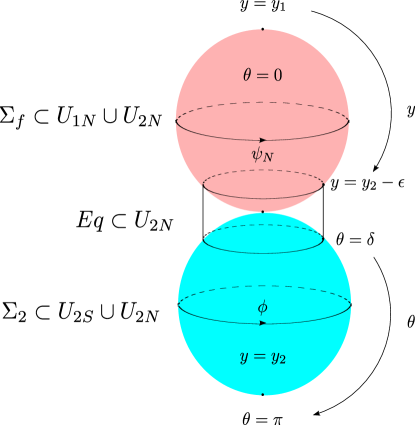
Figure 1: Desingularisation of $\Sigma_{2}\cup-\Sigma_{f}$.

We first examine the overlaps

$$\frac{q(p+q)}{l_{v}}\left[A^{\prime}_{2N}-A^{\prime}_{1N}\right] = -aq(p+q)d\psi_{N}=q((b-a)q-1)d\psi_{N}$$

$$\frac{q(p+q)}{l_{v}}\left[A^{\prime}_{2S}-A^{\prime}_{2N}\right] = -bq(p+q)d\phi=-q((b-a)p+1)d\phi~{}.$$ (3.29)

This leads us to define

$$\frac{q(p+q)}{l_{v}}\tilde{A}^{\prime}_{2N}=\frac{q(p+q)}{l_{v}}{A}^{\prime}_{2N}+qd\psi_{N}-q(b-a)\frac{dw_{2N}}{l_{w}}~{},$$ (3.30)

which is obtained via a good gauge transformation on this patch. We then find

$$\frac{q(p+q)}{l_{v}}\left[\tilde{A}^{\prime}_{2N}-A^{\prime}_{1N}\right] = q^{2}(b-a)d\psi_{N}-q(b-a)\frac{dw_{2N}}{l_{w}}$$ (3.31)

$$= -q(b-a)\frac{dw_{1N}}{l_{w}}$$

$$\frac{q(p+q)}{l_{v}}\left[A^{\prime}_{2S}-\tilde{A}^{\prime}_{2N}\right] = -pq(b-a)d\phi+q(b-a)\frac{dw_{2N}}{l_{w}}$$ (3.32)

$$= q(b-a)\frac{dw_{2S}}{l_{w}}~{}.$$

This prompts us to define

$$\frac{q(p+q)}{l_{v}}\tilde{A}^{\prime}_{1N} = \frac{q(p+q)}{l_{v}}{A}^{\prime}_{1N}-q(b-a)\frac{dw_{1N}}{l_{w}}$$

$$\frac{q(p+q)}{l_{v}}\tilde{A}^{\prime}_{2S} = \frac{q(p+q)}{l_{v}}{A}^{\prime}_{2S}-q(b-a)\frac{dw_{2S}}{l_{w}}~{},$$ (3.33)

which are again obtained via good gauge transformations on the patches. After all this, $\tilde{A}^{\prime}$ is a globally defined one-form on $F_{1}$, and thus we see explicitly that the $v$ bundle trivialises over it since we have divided the period by $(p+q)q$. Moreover, one finds that $a$ and $b$ end up completely cancelling, and that the correct connection form to use on $U_{1N}$ and $U_{2S}$ is

$$\tilde{A}^{\prime}_{1N} = -A_{v}(y_{1})d\psi_{N}+A_{v}D\psi_{N}-\frac{l_{v}}{2q(p+q)}\frac{dw_{1N}}{l_{w}}$$

$$\tilde{A}^{\prime}_{2S} = -A_{v}(y_{2})d\psi_{S}+A_{v}D\psi_{S}-\frac{l_{v}}{2q(p+q)}\frac{dw_{1S}}{l_{w}}~{}.$$ (3.34)

By taking $\epsilon,\delta\to 0$ we effectively use the gauge $\tilde{A}^{\prime}_{1N}$ over $E_{f}$ and $\tilde{A}^{\prime}_{2S}$ over $E_{2}$ and then consider the result for $E_{2}$ minus the result for $E_{f}$. After some calculation this gives the period

$$\frac{1}{(2\pi l_{s})^{2}g_{s}}\int_{V_{1}}F^{(3)}=-\frac{L^{2}}{l_{s}^{2}g_{s}}\frac{(p+q)^{3}}{pq^{2}(p+2q)}\equiv-\frac{M_{1}}{p+q}~{},$$ (3.35)

where $M_{1}$ is a positive integer.

Consistency of (3.27) and (3.35) implies that we choose

$$M_{1}=M(p+q)^{2},\qquad M_{2}=Mq^{2}$$ (3.36)

for some positive integer $M$ and

$$\frac{{L}^{2}}{l_{s}^{2}g_{s}}=\frac{pq^{2}(p+2q)M}{(p+q)^{2}}~{}.$$ (3.37)

We have thus recovered the results (3.8) and (3.1), which is very satisfying.

3.3 Taking the limit $Q\to 0$

We have noted that the parameter $Q\neq 0$ corresponds to an exactly marginal deformation of the underlying dual $(0,2)$ SCFT. In particular, the solutions, with the internal manifold having topology $S^{3}\times S^{3}\times S^{1}$, and all other parameters fixed, are smoothly connected with each other as $Q$ varies and they all have the same central charge. It is interesting to observe that the value of the central charge is precisely the same as for the solutions with $Q=0$ that were analysed in [26]. It is therefore tempting to conclude that the solutions with $Q\neq 0$ correspond to exactly marginal deformations of the SCFTS dual to the $Q=0$ solutions. While this may in fact be the correct interpretation, it seems difficult to draw this conclusion based on the results of this paper. In particular, taking the limit $Q\to 0$ does not simply lead to the $Q=0$ solutions discussed in [26], as we now explain.

It is certainly the case that setting $Q$ to zero in the local solutions given by (2.1), (2.2), (2.8) and (2.9) one obtains the local solutions with $Q=0$ studied in [26]. However, we also need to check what happens to the global identifications we have made on the coordinates, and also the quantisation of the flux. Recall that in the solutions of [26] with $Q=0$ the internal manifold has topology $S^{2}\times S^{3}\times T^{2}$, with the $S^{2}\times S^{3}$ factor realised in the same way as the $M_{5}$ factor for the $Q\neq 0$ solutions studied here. It is simple to check that taking the limit $Q\to 0$ in the spaces $B_{4}$ and $M_{5}$, labeled by $p,q$, studied in sections 2.2 and 2.3, respectively, leads to the corresponding spaces in the $Q=0$ solutions of [26]. The problem arises in taking the limit of the $v$ circle fibration. In (2.46) we impose that this has twist 1 over the base $M_{5}=S^{2}\times S^{3}$. This is impossible as $Q\to 0$, because the connection $A_{v}\to 0$ and correspondingly, the period $l_{v}$ goes to zero in (2.47). From (2.1) we therefore conclude that the period of the $u^{1}$ circle goes to zero in this limit and we do not match onto the $Q=0$ solutions of [26] where the $u^{1}$ circle in the $T^{2}$ factor had finite period.

It is worth pointing out that in the $Q=0$ solutions of [26], with topology $S^{2}\times S^{3}\times T^{2}$, only the volume of the $T^{2}$ was fixed by the flux quantisation. The shape of the $T^{2}$ therefore corresponds to exactly marginal deformations. It might be the case that going to the limit where the period of the $u^{1}$ circle goes to zero is connected to the $Q\to 0$ limiting solutions. However, in this limit the supergravity approximation is clearly breaking down and one needs to analyse string corrections before any definite conclusions can be drawn. It would be interesting to study this further.

4 More general identifications

In this section we will generalise the class of solutions that we have already constructed. We return to the local solution (2.1), (2.8), (2.1) and then employ the general linear coordinate transformation

$$w= h\,w^{\prime}+r\frac{Q}{Z}\,v^{\prime}$$

$$v= s\,w^{\prime}+\frac{t}{2\beta}\,v^{\prime}$$ (4.1)

for constant $r,t,s,h$ with

$$\Delta=h\frac{t}{2\beta}-r\frac{Q}{Z}s\neq 0~{}.$$ (4.2)

The idea is to now make appropriate periodic identifications of the new coordinates $v^{\prime},w^{\prime}$. As we shall see this will embed our solutions of type IIB string string theory of the last two sections into larger families.

We first observe that

$$Dw = h\,Dw^{\prime}+r\frac{Q}{Z}\,Dv^{\prime}$$

$$Dv = s\,Dw^{\prime}+\frac{t}{2\beta}\,Dv^{\prime}$$ (4.3)

where we have defined

$$Dw^{\prime} = dw^{\prime}-A_{w^{\prime}}\,D\psi$$

$$Dv^{\prime} = dv^{\prime}-A_{v^{\prime}}\,D\psi$$ (4.4)

with

$$A_{w^{\prime}} = \frac{t}{2\beta\Delta}\,A_{w}-r\frac{Q}{Z\Delta}\,A_{v}$$

$$A_{v^{\prime}} = \frac{h}{\Delta}\,A_{v}-\frac{s}{\Delta}\,A_{w}~{}.$$ (4.5)

We now construct $M_{5}$ as a circle fibration, with circle parametrised by $w^{\prime}$, over $B_{4}$ and then construct $M_{6}$ as a circle fibration, with circle parametrised by $v^{\prime}$, over $M_{5}$. It is straightforward to write the metric in the primed coordinates and then appropriately “complete the square” to make this fibration structure manifest in the metric. However, we will not need the explicit details. Observe that what will become the globally defined angular one-form on $M_{5}$ for the $w^{\prime}$ circle fibration is $Dw^{\prime}$. After completing the square in the metric on $M_{6}$ we obtain an expression for what will become the globally defined angular one-form corresponding to the $v^{\prime}$ circle fibration and it has the form

$$dv-A_{v^{\prime}}D\psi-k(y)Dw^{\prime}$$ (4.6)

for some smooth function $k(y)$ that can easily be determined. The connection one-form on $M_{5}$ for this circle fibration is thus $A_{v^{\prime}}D\psi+k(y)Dw^{\prime}$. This will turn out to be a local connection one-form on the same circle bundle as that for the connection one-form $A_{v^{\prime}}D\psi$, since $kDw^{\prime}$ will be globally defined on $M_{5}$ (in particular, the corresponding curvature two-forms are in the same cohomology class on $M_{5}$). Below, for convenience, we will use the connection one-form $A_{v^{\prime}}D\psi$.

The analysis now proceeds in an almost identical fashion as in the last sections, so we can be brief. We choose the period of the $w^{\prime}$ circle to be $2\pi l_{w^{\prime}}$ so that $l_{w^{\prime}}^{-1}A_{w^{\prime}}D\psi$ is a connection on a $U(1)$ fibration. We demand that $(2\pi l_{w})^{-1}d(A_{w}\,D\psi)$ has integer periods on $B_{4}$, as in (2.3), with primes on all $w$, for some integers $p,q$, now not necessarily positive. When $r+t=0$ we have $q=0$, while when $r-t=0$ we have $p+q=0$ and these cases require a separate analysis which we will return to later. We thus continue here with $r\neq\pm t$ and conclude that

$$\beta = \frac{t-r}{t+r}\frac{q}{p+q}$$

$$l_{w^{\prime}} = \frac{(2-Z)(r+t)}{2q(1-Z)(1-\beta^{2})\Delta}$$ (4.7)

The topology of $M_{5}$ is again $S^{3}\times S^{2}$. For the generator of $H^{3}\left(M_{5},\mathbb{Z}\right)$ we can use the primed version of (2.3).

We now turn to the $v^{\prime}$ circle fibration over $M_{5}$ to give $M_{6}$. We let $v^{\prime}$ be a periodic coordinate with period $2\pi l_{v^{\prime}}$, and the connection one-form is given by $l_{v^{\prime}}^{-1}A_{v^{\prime}}D\psi$. To ensure that the circle fibration is well-defined and that $M_{6}=S^{3}\times S^{3}$ we impose the primed version of (2.46) to conclude that

$$l_{v^{\prime}}=\frac{2qQ}{\left(r+t\right)\left(1-Z\right)}.$$ (4.8)

Now we determine the flux quantisation conditions. The electric flux quantisation condition (3.1) fixes the period of $u^{2}$ as before:

$$n_{1}=\frac{L^{6}}{l_{s}^{6}g_{s}}\frac{Q}{8\pi^{2}\beta(1-\beta^{2})^{2}}\Delta u^{2}~{}.$$ (4.9)

For the magnetic flux quantisation, we follow the same procedure as before, by introducing explicit coordinate patches and considering integrals on submanifolds of $\hat{M}_{6}=M_{6}/{\mathbb{Z}}_{(p+q)q}$. By following the same steps as in section 3.2 we find that

$$\frac{1}{\left(2\pi l_{s}\right)^{2}g_{s}}\int_{V_{2}}F^{(3)} = \frac{L^{2}}{l_{s}^{2}g_{s}}\frac{1}{q}\frac{1}{\beta^{2}-1}\equiv-\frac{M_{2}}{q}$$

$$\frac{1}{\left(2\pi l_{s}\right)^{2}g_{s}}\int_{V_{1}}F^{\left(3\right)} = \frac{L^{2}}{l_{s}^{2}g_{s}}\frac{1}{q}\frac{r+t}{r-t}\frac{1}{\beta\left(1-\beta^{2}\right)}\equiv-\frac{M_{1}}{p+q}$$ (4.10)

for integers $M_{2},M_{1}$. Consistency implies that we must have

$$\frac{M_{2}}{M_{1}}=\beta^{2}=\frac{(r-t)^{2}}{(r+t)^{2}}\frac{q^{2}}{(p+q)^{2}},$$ (4.11)

which implies that $(r+t)^{2}/(r-t)^{2}$ must be rational, and that the length scale is fixed by

$$\frac{L^{2}}{l_{s}^{2}g_{s}}=(1-\beta^{2})M_{2}=\frac{(M_{1}-M_{2})M_{2}}{M_{1}}$$ (4.12)

The central charge can now be calculated, and we find that it can be expressed as

$$c=6n_{1}\frac{(M_{1}-M_{2})M_{2}}{M_{1}}~{}.$$ (4.13)

In particular we note that, in addition to $Q$, there is also no dependence on the parameters $r,s,t$ and $h$. We note that the only restrictions on these parameters is (4.2), (4.11) with $\beta$ given in (4) satisfying $0<\beta<1$. We have thus constructed large continuous families of solutions that are dual to SCFTs. Note that, in general, the solutions of this section are not exactly marginal deformations of those in section 3: for example, in section 3 we saw that the magnetic three-form flux quantum numbers were constrained to be of the form (3.36), whereas here there is no such constraint.

When $r=-t$:

When $r=-t$, we have $A_{w^{\prime}}(y_{1})=A_{w^{\prime}}(y_{2})$ and hence in considering the $w^{\prime}$ circle fibration over $B_{4}$ to construct $M_{5}$ we find that the period over $C_{2}=\Sigma_{f}$ vanishes, $q=0$. We choose $p=1$, so that the period over $C_{1}=\Sigma_{2}-\Sigma_{f}$ is one, and hence $M_{5}=S^{3}\times S^{2}$, which implies that

$$l_{w^{\prime}}=2A_{w^{\prime}}(y_{2})=-\frac{t(Z-2)}{\beta(\beta^{2}-1)(Z-1)\Delta}~{}.$$ (4.14)

At this stage, there is no restriction on the parameter $\beta$ (apart from the usual $0<\beta<1$). We now find on $M_{5}$ that $E_{1},E_{2}\cong S^{3}$, and $[E_{1}]=[E_{2}]$ generate $H_{3}(M_{5},{\mathbb{Z}})$. On the other hand, now $E_{f}\cong S^{1}\times S^{2}$ (and hence there is a section of the $w^{\prime}$ circle fibration over $\Sigma_{f}$). The generator of $H^{2}(M_{5},{\mathbb{Z}})$ is $\tau=\sigma_{f}$ i.e. $a=1,b=0$, in the notation of section 2.3.

In order to construct $M_{6}=S^{3}\times S^{3}$, we can again fix the period of the $v^{\prime}$ circle using $\Phi$ as in (2.46) and we find that

$$l_{v^{\prime}}=A_{v^{\prime}}(y_{2})-A_{v^{\prime}}(y_{1})=-\frac{\beta Q}{(Z-1)t}~{}.$$ (4.15)

It is now easier to find representatives of the two generators of $H_{3}(M_{6},{\mathbb{Z}})$, and we won’t have to consider a quotient of $M_{6}$ in order to impose the flux quantisation conditions. In particular, one generator of $H_{3}(M_{6},{\mathbb{Z}})$, $W_{1}$, can be taken to be, as above, the section of the $v^{\prime}$ circle fibration over a desingularised version of $E_{2}\cup-E_{f}$. For the other generator, $W_{2}$, we can take the $v^{\prime}$ circle bundle over the section $s(S)$ on $M_{5}$ where $S=\Sigma_{f}$. We note that two other three-cycles $W^{\prime}$, $W^{\prime\prime}$ are obtained by considering a section of the $v^{\prime}$ circle fibration over $E_{1}$, $E_{2}$, respectively: we shall show that $[W^{\prime}]=[W^{\prime\prime}]=[W_{1}]+[W_{2}]$.

We now introduce patches in exactly the same way as section 3.2. The analogue of (3.17) now reads $w^{\prime}_{2N}=w^{\prime}_{1N}$ and we explicitly see that the $w^{\prime}$ circle fibration is indeed trivial over $\Sigma_{f}$. To obtain the section $s[\Sigma_{f}]$ we can simply set $w^{\prime}_{2N}=constant$.

Moving to $M_{6}$, we have the analogue of the connection one-forms as in (3.2), (3.2) with $a=1$, $b=0$, $p=1$, $q=0$. Equation (3.22) shows that the $v^{\prime}$ circle fibration is indeed trivial over $E_{2}$ and we can take a section to obtain the three-cycle $W^{\prime\prime}$. One can then obtain the integral of the three-form flux over $W^{\prime\prime}$ by using the connection one form $A^{\prime}_{2N}$, and after a calculation we find

$$\frac{1}{\left(2\pi l_{s}\right)^{2}g_{s}}\int_{W^{\prime\prime}}F^{\left(3\right)}=-\frac{L^{2}}{l_{s}^{2}g_{s}}\frac{1}{\beta^{2}}~{}.$$ (4.16)

The $v^{\prime}$ circle fibration is also trivial over $E_{1}$. Indeed, after considering (3.22) we can see that the connection one-form

$$A^{\prime}_{1S}+2l_{v^{\prime}}\frac{dw^{\prime}_{1s}}{l_{w^{\prime}}}$$ (4.17)

is a globally defined one-form on $E_{1}$. We can use this gauge to calculate the integral over $W^{\prime}$ and we find exactly the same result as for $W^{\prime\prime}$.

To calculate the integral of the flux over the three-cycle $W_{2}$, the $v^{\prime}$ circle bundle over the section $s(\Sigma_{f})$, we just need to set $w^{\prime}_{2N}=constant$ in the expression for the three-form and then integrate. We therefore impose

$$\frac{1}{\left(2\pi l_{s}\right)^{2}g_{s}}\int_{W_{2}}F^{\left(3\right)}=\frac{L^{2}}{l_{s}^{2}g_{s}}\frac{1}{\left(1-\beta^{2}\right)}=M_{2}~{}.$$ (4.18)

To carry out the flux integral over $W_{1}$, a section of the $v^{\prime}$ circle fibration over $E_{2}\cup-E_{f}$, we define

$$\frac{1}{l_{v^{\prime}}}\tilde{A}_{2N}^{\prime} = \frac{1}{l_{v^{\prime}}}A_{2N}^{\prime}+d\psi_{N}+\frac{dw_{2N}}{l_{w}}$$

$$\frac{1}{l_{v^{\prime}}}\tilde{A}_{1N}^{\prime} = \frac{1}{l_{v^{\prime}}}A_{1N}^{\prime}+\frac{dw_{1N}}{l_{w}}$$

$$\frac{1}{l_{v^{\prime}}}\tilde{A}_{2S}^{\prime} = \frac{1}{l_{v^{\prime}}}A_{2S}^{\prime}+\frac{dw_{2S}}{l_{w}}~{}.$$ (4.19)

Then $\tilde{A}^{\prime}$ is a global one-form on $E_{2}\cup-E_{f}$. To calculate the integral of flux over the section over the $v^{\prime}$ circle bundle over $E_{2}\cup-E_{f}$ we use $\tilde{A}_{2S}^{\prime}$ on $E_{2}$ and $\tilde{A}_{1N}^{\prime}$ on $E_{f}$. We find

$$\frac{1}{\left(2\pi l_{s}\right)^{2}g_{s}}\int_{W_{1}}F^{\left(3\right)}=-\frac{L^{2}}{l_{s}^{2}g_{s}}\frac{1}{\beta^{2}\left(1-\beta^{2}\right)}=-M_{1}~{}.$$ (4.20)

Comparing (4.16) with (4.18) and (4.20), we can deduce the homology relation $[W^{\prime\prime}]=[W^{\prime}]=[W_{1}]+[W_{2}]$, as mentioned above.

Consistency of (4.18) and (4.20) implies that the length scale of the solution is again as in (4.12) and that $\beta^{2}$ is rational

$$\beta^{2}=\frac{M_{2}}{M_{1}}~{}.$$ (4.21)

The electric flux quantisation condition is given again by (4.9) and the central charge takes the form (4.13).

When $r=t$:

When $r=t$, we have $A_{w^{\prime}}(y_{1})=-A_{w^{\prime}}(y_{2})$ and hence in considering the $w^{\prime}$ circle fibration over $B_{4}$ to construct $M_{5}$ we find that the period over $C_{1}=\Sigma_{2}-\Sigma_{f}$ vanishes, $p+q=0$. We choose $q=1$ so that the period over $C_{2}=\Sigma_{f}$ is one, and hence $M_{5}=S^{3}\times S^{2}$, which implies that

$$l_{w^{\prime}}=\frac{-t(Z-2)}{(\beta^{2}-1)(Z-1)\Delta}$$ (4.22)

with no restriction on the parameter $\beta$. We now find $E_{1},E_{2},E_{f}\cong S^{3}$, and $-[E_{1}]=[E_{2}]=[E_{f}]$ generate $H_{3}(M_{5},{\mathbb{Z}})$. The generator of $H^{2}(M_{5},{\mathbb{Z}})$ is $\tau=b\sigma_{2}+a\sigma_{f}$ with $b-a=1$.

In order to construct $M_{6}=S^{3}\times S^{3}$, we find that the period of the $v^{\prime}$ circle is

$$l_{v^{\prime}}=A_{v^{\prime}}(y_{1})+A_{v^{\prime}}(y_{2})=-\frac{Q}{(Z-1)t}~{}.$$ (4.23)

For the generators of $H_{3}(M_{6},{\mathbb{Z}})$ we can take $W_{1}$ to be the $v^{\prime}$ circle fibration over the a representative of the section $s(S)$ of $M_{5}$, with $[S]=[\Sigma_{2}]-[\Sigma_{f}]$. For $W_{2}$ we take a section of the $v^{\prime}$ circle fibration over $E_{f}$. We note that we can also obtain three-cycles $W^{\prime}$, $W^{\prime\prime}$ which are obtained by considering sections of the $v^{\prime}$ circle fibration over $E_{1}$, $E_{2}$ respectively: we shall see that $-[W^{\prime}]=[W^{\prime\prime}]=[W_{1}]+[W_{2}]$.

We again introduce patches in exactly the same way as section 3.2. The connection one-forms are as in (3.2), (3.2) with $b-a=1$ and $q=-p=1$. By taking $a=0$, $b=1$, we see from (3.21) that $A^{\prime}_{2N}$ is a globally defined connection one-form on $E_{f}$. Calculating the flux integral we find that we should impose

$$\frac{1}{\left(2\pi l_{s}\right)^{2}g_{s}}\int_{W_{2}}F^{\left(3\right)}=-\frac{L^{2}}{l_{s}^{2}g_{s}}\frac{1}{\left(1-\beta^{2}\right)}=-M_{2}~{}.$$ (4.24)

To integrate the flux integrals for $W^{\prime}$ one should take $b=2$, $a=1$ while for $W^{\prime\prime}$ we should take $b=0$, $a=-1$ and we find

$$-\frac{1}{\left(2\pi l_{s}\right)^{2}g_{s}}\int_{W^{\prime}}F^{\left(3\right)}=\frac{1}{\left(2\pi l_{s}\right)^{2}g_{s}}\int_{W^{\prime\prime}}F^{\left(3\right)}=\frac{L^{2}}{l_{s}^{2}g_{s}}\frac{1}{\beta^{2}}~{}.$$ (4.25)

We now turn to the flux integral over $W_{1}$. For $S$ we desingularise $\Sigma_{2}-\Sigma_{f}$ as in Figure 1. By making the gauge transformation $w^{\prime}_{2N}\to w^{\prime}_{2N}-l_{w^{\prime}}d\psi_{N}$ in (3.15), we find that we obtain a globally defined connection one-form on $S\subset M_{5}$ and hence we can take a section. $W_{1}$ is obtained by considering the $v^{\prime}$ circle fibration over this section. Thus to calculate the flux integral, one should set $w^{\prime}_{1N}=constant$ in $Dw^{\prime}_{1N}$ for the $\Sigma_{2}$ piece and $w^{\prime}_{1S}=constant$ in $Dw^{\prime}_{1S}$ for the $\Sigma_{f}$ piece. After doing this we find

$$\frac{1}{\left(2\pi l_{s}\right)^{2}g_{s}}\int_{W_{1}}F^{\left(3\right)}=-\frac{L^{2}}{l_{s}^{2}g_{s}}\frac{1}{\beta^{2}\left(1-\beta^{2}\right)}=-M_{1}~{}.$$ (4.26)

We thus find the same conditions as for the $r=-t$ case above.

5 Final Comments

We have analysed in detail some local supersymmetric $AdS_{3}$ solutions of type IIB supergravity, first found in [26], that have non-vanishing dilaton and $RR$ three-form flux. We have shown that the parameters can be chosen and coordinates identified in such a way that the solutions extend to give rich classes of globally defined solutions of the form $AdS_{3}\times_{w}(S^{3}\times S^{3}\times S^{1})$ with properly quantised flux. We have shown that the solutions depend on continuous parameters and are hence dual to continuous families of SCFTs in two spacetime dimensions with $(0,2)$ supersymmetry.

Although the internal compact spaces are diffeomorphic to $S^{3}\times S^{3}\times S^{1}$, the diffeomorphisms are far from apparent in the local coordinates that the solutions are presented in. It seems unlikely to us that there is a simple change of coordinates that will make the topology more manifest. In this paper we used a number of techniques to illuminate various aspects of the topology which, in particular, allowed us to find a workable procedure to impose flux quantisation. It seems likely that our approach, or generalisations thereof, will be very useful in other contexts.

In section 4 we considered identifications on the coordinates after we made a general linear transformation on the $v,w$ coordinates. It is worth pointing out that we could consider more general linear coordinate transformations that also involve the $u^{2}$ coordinate. This will lead to larger families of solutions that would be worth exploring. It seems possible that some of these solutions can be obtained as $\beta$-deformations using the techniques of [38]. In fact returning to the solutions in section 2 and 3, one might wonder if $Q$ corresponds to a $\beta$-deformation. One way to see that it is not is to return to the local solutions as written down at the beginning of section 4 of [26], which are obtained after two T-dualities on the solutions we have discussed in this paper. In this duality frame only the metric and the self-dual five-form are non-trivial for any $Q$, and in particular the dilaton is constant. However, looking at equation (A.16) of [38] we see that the $\beta$-deformation activates a non-trivial dilaton and three-form.

It is an important outstanding issue to identify the dual $(0,2)$ SCFTs for the solutions discussed here and in [24, 14, 25, 26]. In the duality frame that we have used in this paper, the amount of supersymmetry that is preserved combined with the fluxes that are active suggests that the dual SCFTs might arise on a D1-D5-brane system that is wrapped on a holomorphic four-cycle in a Calabi-Yau four-fold. While we remain hopeful that progress will be made in this direction, we note that the SCFTs dual to the much simpler type IIB $AdS_{3}\times S^{3}\times S^{3}\times S^{1}$ solutions of [32], which have $(4,4)$ supersymmetry, are still not well-understood, despite interesting progress [33, 34, 35, 36].

The $AdS_{3}$ solutions with $Q=0$, that were analysed in [26], and with $Q\neq 0$ that we have discussed here, can be generalised further and we have presented some details in appendix C. It will be interesting to carry out a complete analysis of the conditions for regularity and flux quantisation conditions for these more general solutions.

Acknowledgements

We would like to thank Jaume Gomis, Dominic Joyce, Spiro Karigiannis, Nakwoo Kim, Tommaso Pacini and David Tong for helpful discussions, and Bob McNees for help with Inkscape. We would also like to thank one of the referees for insightful comments which led to the discussion in section 3.3. AD would also like to thank the Institute for Mathematical Sciences at Imperial College for hospitality. JPG would like to thank the Perimeter Institute for hospitality. JPG is supported by an EPSRC Senior Fellowship and a Royal Society Wolfson Award. JFS is supported by a Royal Society University Research Fellowship.

Appendix A $U(1)$ bundles over Lens spaces

In this section we briefly review the Lens spaces $S^{3}/{\mathbb{Z}}_{q}$, which appear throughout the main text, and also the construction of $U(1)$ principal bundles over these manifolds.

We construct $S^{3}/{\mathbb{Z}}_{q}$ as the total space of a $U(1)$ bundle over $S^{2}$ with Chern number $q$. Let $\theta$, $\phi$ be standard coordinates on $S^{2}$, and cover the $S^{2}$ with two patches: $V_{N}$ which excludes the south pole $\theta=\pi$, and $V_{S}$ which excludes the north pole $\theta=0$. We then consider the products $S^{1}\times V_{N}$, $S^{1}\times V_{S}$, and on each space define the one-forms

$$D\nu_{N} = d\nu_{N}-\frac{q}{2}(1-\cos\theta)d\phi$$

$$D\nu_{S} = d\nu_{S}+\frac{q}{2}(1+\cos\theta)d\phi~{}.$$ (A.1)

Here $\nu_{N}$ and $\nu_{S}$ are coordinates on the $S^{1}s$, each with period $2\pi$. If we now glue the two patches together via

$$\nu_{S}-\nu_{N}=-q\phi$$ (A.2)

on the overlap then note that

$$D\nu=D\nu_{N}=D\nu_{S}$$ (A.3)

extends to a global one-form on the whole manifold, because the two one-forms agree on the overlap. This is a global connection form on the total space of the $U(1)$ principal bundle $\mathrm{p}:S^{3}/{\mathbb{Z}}_{q}\rightarrow S^{2}$ with $U(1)$ fibre parametrised by $\nu$, and is sometimes also called the global angular form.

Now consider the connection form

$$A_{N} = \frac{a}{2}(1-\cos\theta)d\phi$$

$$A_{S} = -\frac{a}{2}(1+\cos\theta)d\phi$$ (A.4)

on the base $S^{2}$. This has Chern number $a\in{\mathbb{Z}}$ over the base $S^{2}$. We denote the corresponding $U(1)$ principal bundle by $P$. We may pull back $P$ to a $U(1)$ bundle $\mathrm{p}^{*}P$ over $S^{3}/{\mathbb{Z}}_{q}$. Pulling back the connection (A), on the overlap one finds

$$A_{S}-A_{N}=-ad\phi=\frac{a}{q}d(\nu_{S}-\nu_{N})~{}.$$ (A.5)

Note that $a\nu_{S}/q$ is a multi-valued $U(1)$ function on the patch $S^{1}\times V_{S}$ unless $a/q\in{\mathbb{Z}}$. If $a/q\in{\mathbb{Z}}$ then in each patch we can define the new connection one-forms $A_{S}-ad\nu_{S}/q$ and $A_{N}-ad\nu_{N}/q$, and since they agree on the overlap, this defines a globally defined connection one-form and hence $\mathrm{p}^{*}P$ is trivial.

Thus $\mathrm{p}^{*}P$ is trivial if and only if $a\cong 0$ mod $q$. One sees this in a more abstract way by recalling that $U(1)$ principal bundles are classified by $H^{2}(S^{3}/{\mathbb{Z}}_{q},{\mathbb{Z}})\cong H_{1}(S^{3}/{\mathbb{Z}}_{q},{\mathbb{Z}})\cong{\mathbb{Z}}_{q}$. Thus $a\in{\mathbb{Z}}_{q}$ is precisely the Chern number of $\mathrm{p}^{*}P$, and the latter bundle is torsion. Because of this, the topology cannot be measured by integrating the curvature of a connection $A$ over a two-cycle – to see torsion classes using the connection is more subtle. This is explained in general in the paper [37]. The latter reference implies that the torsion first Chern class may be computed by picking a flat connection on $\mathrm{p}^{*}P$, and then computing the log of the holonomy of this flat connection around the one-cycles that generate $H_{1}(S^{3}/{\mathbb{Z}}_{q},{\mathbb{Z}})$. We may shift to a flat connection here by defining

$$A_{S}^{\mathrm{flat}} = A_{S}+\frac{a}{q}D\nu_{S}=\frac{a}{q}d\nu_{S}$$

$$A_{N}^{\mathrm{flat}} = A_{N}+\frac{a}{q}D\nu_{N}=\frac{a}{q}d\nu_{N}$$ (A.6)

Here we have added a global one-form $(a/q)D\nu$ to the original connection – we are simply picking a different connection on the same bundle. Then $H_{1}(S^{3}/{\mathbb{Z}}_{q},{\mathbb{Z}})\cong{\mathbb{Z}}_{q}$ is generated by, for example, the $\psi_{N}$ circle at $\theta=0$. Thus the log of the holonomy is

$$i\int_{S^{1}}A_{N}^{\mathrm{flat}}=\frac{2\pi ia}{q}\quad\mathrm{mod}\ 2\pi i~{}.$$ (A.7)

This implies that our connection above is $a$ times the generator of ${\mathbb{Z}}_{q}$.

Finally, we make a comment about quotients. First note that quotienting the period of the $U(1)$ fibre coordinate of $P$ by $q$ is the same as taking the $q$th power of $P$. In particular, the ${\mathbb{Z}}_{q}$ quotient of the bundle $\mathrm{p}^{*}P$ over $S^{3}/{\mathbb{Z}}_{q}$ is then trivial. This follows simply because the connection on this bundle in the two patches is $qA_{S}$ and $qA_{N}$, or after a gauge transformation $qA_{S}-ad\nu_{S}$ and $qA_{N}-ad\nu_{N}$, and from (A.5) we see that this is a globally defined connection one-form, and hence the bundle is trivial.

Appendix B More on the topology of $M_{5}$

Recall that, in the main text, $M_{6}$ is constructed as the total space of a circle bundle $L$ over $M_{5}\cong S^{3}\times S^{2}$. Here $c_{1}(L)\in H^{2}(M_{5},{\mathbb{Z}})\cong{\mathbb{Z}}$ is the generator, so that $M_{6}\cong S^{3}\times S^{3}$. Although this is straightforward as stated, the issue is that we have infinitely many coordinate systems on $M_{5}$, labelled by the integers $p$ and $q$, and the diffeomorphism $M_{5}\cong S^{3}\times S^{2}$ is not explicit for general $p$ and $q$. For each $p$ and $q$ there are different naturally-defined three-submanifolds of $M_{5}$ – we are especially interested in three-submanifolds since we would like to quantise the RR three-form flux. In this appendix we consider these submanifolds in more detail, and in particular determine the topology of $L$ restricted to them.

Consider restricting this circle bundle $L$ over $M_{5}$ to one of the three-submanifolds of $M_{5}$: $E_{1}$, $E_{2}$ or $E_{f}$. For example, take $E_{f}\cong S^{3}/{\mathbb{Z}}_{q}$. Recall this is itself a circle bundle over $\Sigma_{f}\cong S^{2}$ with Chern class $q$. There is an inclusion map $i_{f}:E_{f}\hookrightarrow M_{5}$, and we can define a circle bundle $L_{f}$ over $E_{f}$ by pulling back

$$L_{f}\equiv i_{f}^{*}L~{}.$$ (B.1)

Since $E_{f}$ is a lens space, $E_{f}=S^{3}/{\mathbb{Z}}_{q}$, circle bundles over $E_{f}$ are classified up to isomorphism by

$$c_{1}(L_{f})\in H^{2}(E_{f},{\mathbb{Z}})\cong{\mathbb{Z}}_{q}~{}.$$ (B.2)

To compute this Chern class, recall that $c_{1}(L)=\pi^{*}\tau$, where $\tau\in H^{2}(B_{4},{\mathbb{Z}})$ was defined in (2.34). Hence to compute $c_{1}(L_{f})=i^{*}_{f}\pi^{*}(\tau)$ we may instead first restrict $\tau$ to $\Sigma_{f}$, and then pull back using $\pi^{*}$ the corresponding circle bundle to $E_{f}$. This is summarised by the following commutative square:

$$\begin{array}[]{ccc}H^{2}(M_{5},{\mathbb{Z}})&\stackrel{{\scriptstyle i_{f}^{*}}}{{\longrightarrow}}&H^{2}(E_{f},{\mathbb{Z}})\\ \pi^{*}\big{\uparrow}&&\big{\uparrow}\pi^{*}\\ H^{2}(B_{4},{\mathbb{Z}})&\stackrel{{\scriptstyle\iota_{f}^{*}}}{{\longrightarrow}}&H^{2}(\Sigma_{f},{\mathbb{Z}})\end{array}~{}.$$ (B.6)

Here we have denoted the embedding of $\Sigma_{f}$ into $B_{4}$ by $\iota_{f}:\Sigma_{f}\rightarrow B_{4}$. Then $\iota_{f}^{*}\tau$ defines an integer class in $H^{2}(\Sigma_{f},{\mathbb{Z}})\cong{\mathbb{Z}}$. This in turn defines a circle bundle with Chern number $a$, using (2.34). Using the results in appendix A, lifting this circle bundle to $E_{f}$ then gives a bundle with Chern number

$$a=c_{1}(L_{f})\in H^{2}(E_{f},{\mathbb{Z}})\cong{\mathbb{Z}}_{q}~{}.$$ (B.7)

Thus the bundle $L$ restricted to $E_{f}$ is trivialisable only if $a=0$ mod $q$; in other words, if $a=mq$ for some integer $m$. But if this were the case, then we would have

$$(mp+b)q=1~{}.$$ (B.8)

This is only possible if $q=\pm 1$. Thus we see that for general $q$ it is not possible to take a section of $L$ over $E_{f}$ to obtain a three-submanifold of $M_{6}$.

One can do similar computations for the three-submanifolds $E_{1}$ and $E_{2}$, with similar conclusions. We have

$$L_{1}\equiv i^{*}_{1}L \qquad c_{1}(L_{1})=b-2a\in H^{2}(E_{1},{\mathbb{Z}})\cong{\mathbb{Z}}_{p+2q}$$ , (B.9)

$$L_{2}\equiv i^{*}_{2}L \qquad c_{1}(L_{2})=b\qquad\ \in H^{2}(E_{2},{\mathbb{Z}})\cong{\mathbb{Z}}_{p}~{}.$$ , (B.10)

Thus the corresponding bundles are trivial if and only if $b=m_{2}p$, $b-2a=m_{1}(p+2q)$, respectively, where $m_{1},m_{2}\in{\mathbb{Z}}$, which implies

$$p(a+qm_{2}) = 1$$

$$(p+2q)(a+m_{1}q) = 1$$ (B.11)

respectively. These equations imply in particular that $p=\pm 1$ and $(p+2q)=\pm 1$.

We thus conclude that, for generic $p$ and $q$, the circle bundle $L$ restricted to $E_{1}$, $E_{2}$ and $E_{f}$ is non-trivial, and thus we cannot globally take a section of $L$. This means that these natural three-submanifolds of $M_{5}$ cannot be used to construct natural three-submanifolds of $M_{6}$.

Appendix C More general $AdS_{3}$ solutions

We first recall from [7], [26] the local data that is sufficient to construct supersymmetric $AdS_{3}$ solutions of type IIB supergravity with non-vanishing five-form flux and complex three-form flux $G$. We require a six-dimensional local Kähler metric $ds^{2}_{6}$ whose Ricci tensor satisfies

$$\Box R-\frac{1}{2}R^{2}+{R}^{ij}{R}_{ij}+\frac{2}{3}G^{ijk}G_{ijk}^{\ast}=0$$ (C.1)

and $G$ must be a closed, primitive and $(1,2)$ three-form on the six-dimensional space. We refer to [7], [26] for details of how the full ten-dimensional solution is constructed from this data.

For the solutions that we have discussed in this paper, which we will now generalise, the local six-dimensional Kahler metric has the form

$$ds^{2}_{6}=ds^{2}_{4}+ds^{2}(T^{2})$$ (C.2)

where $ds^{2}(T^{2})=(du^{1})^{2}+(du^{2})^{2}$ is the standard metric on a two-torus, $ds^{2}_{4}$ is a four-dimensional local Kähler metric, and

$$G=d\bar{u}\wedge W$$ (C.3)

where $u=u^{1}+iu^{2}$ and $W$ is a closed, primitive $(1,1)$-form on the four-dimensional Kähler space.

Inspired by the six-dimensional Kähler metrics discussed in equation 5.10 of [25], we start with the ansatz for a four-dimensional Kähler metric given by

$$ds_{4}^{2} =\frac{Y}{4F}dw^{2}+\sum_{i=1}^{2}\left(w+q_{i}\right)\left(d\mu_{i}^{2}+\mu_{i}^{2}d\phi_{i}^{2}\right)+\frac{F-1}{Y}\left(\sum_{i=1}^{2}\mu_{i}^{2}d\phi_{i}\right)^{2}$$ (C.4)

with

$$\sum_{i=1}^{2}\mu_{i}^{2}=1,\qquad Y=\sum_{i=1}^{2}\frac{\mu_{i}^{2}}{w+q_{i}}$$ (C.5)

and $F$ an arbitrary function of $w$. To show that the metric is Kähler we introduce the orthonormal frame

$$e_{i}= \frac{1}{2\sqrt{F}}\frac{\mu_{i}}{\sqrt{w+q_{i}}}dw+\sqrt{w+q_{i}}d\mu_{i}$$

$$\bar{e}_{i}= \frac{\sqrt{F}-1}{Y}\frac{\mu_{i}}{\sqrt{w+q_{i}}}\sum_{j=1}^{2}\mu_{j}^{2}d\phi_{j}+\sqrt{w+q_{i}}\mu_{i}\,d\phi_{i}$$ (C.6)

with

$$ds_{4}^{2}=\sum_{i=1}^{2}\left(e_{i}\otimes e_{i}+\bar{e}_{i}\otimes\bar{e}_{i}\right).$$ (C.7)

The Kähler form can be written

$$J= \frac{i}{2}\sum_{i=1}^{2}\left(e_{i}-i\bar{e}_{i}\right)\wedge\left(e_{i}+i\bar{e}_{i}\right)=-\sum_{i=1}^{2}e_{i}\wedge\bar{e}_{i}$$

$$= -\frac{1}{2}dw\wedge\sum_{i=1}^{2}\mu_{i}^{2}d\phi_{i}-\sum_{i=1}^{2}\left(w+q_{i}\right)\mu_{i}d\mu_{i}\wedge d\phi_{i}$$ (C.8)

which is clearly closed for any choice of $F$.

The holomorphic $(2,0)$-form $\Omega$ is given by

$$\Omega= \prod_{i=1}^{2}\left(e_{i}-i\bar{e}_{i}\right)$$

$$= \sqrt{w+q_{1}}\sqrt{w+q_{2}}\left[\frac{Y}{2\sqrt{F}}\,dw\wedge d\theta-\sqrt{F}\cos\theta\sin\theta\,d\phi_{1}\wedge d\phi_{2}\right]$$

$$-i\sqrt{w+q_{1}}\sqrt{w+q_{2}}\frac{1}{2\sqrt{F}}\cos\theta\sin\theta\,dw\wedge\left(\frac{d\phi_{2}}{w+q_{1}}-\frac{d\phi_{1}}{w+q_{2}}\right)$$

$$+i\sqrt{w+q_{1}}\sqrt{w+q_{2}}\sqrt{F}\,d\theta\wedge\left(\cos^{2}\theta\,d\phi_{1}+\sin^{2}\theta\,d\phi_{2}\right)$$ (C.9)

where we have introduced $\mu_{1}=\cos\theta$, $\mu_{2}=\sin\theta$, $0<\theta<\frac{\pi}{2}$. A calculation now shows that

$$d\Omega=iP\wedge\Omega$$ (C.10)

with

$$P= \frac{2\sqrt{F}}{Y\sqrt{w+q_{1}}\sqrt{w+q_{2}}}\partial_{w}\left(\sqrt{F}\sqrt{w+q_{1}}\sqrt{w+q_{2}}\right)\,\left(\cos^{2}\theta\,d\phi_{1}+\sin^{2}\theta\,d\phi_{2}\right)$$

$$+\frac{1}{Y}\cos 2\theta\,\left(\frac{d\phi_{2}}{w+q_{1}}-\frac{d\phi_{1}}{w+q_{2}}\right).$$ (C.11)

From this we deduce that the complex structure is integrable, and thus we do indeed have a local Kähler metric with Ricci form given by $dP$. It is helpful to observe that we can also write

$$P= \partial_{w}\left[\left(F-1\right)\left(w+q_{1}\right)\left(w+q_{2}\right)\right]\frac{\sum_{i=1}^{2}\mu_{i}^{2}d\phi_{i}}{Y\left(w+q_{1}\right)\left(w+q_{2}\right)}+d\phi_{1}+d\phi_{2}.$$ (C.12)

We now construct a closed two-form $W$ which satisfies

$$\Omega\wedge W=0,$$ (C.13)

which is the condition for it to be a $\left(1,1\right)$-form, and also

$$J\wedge W=0,$$ (C.14)

which is the condition for it to be a primitive two-form. We make the ansatz

$$W=d\left[f\left(w\right)\,\frac{\sum_{i=1}^{2}\mu_{i}^{2}d\phi_{i}}{Y\left(w+q_{1}\right)\left(w+q_{2}\right)}\right]$$ (C.15)

which satisfies the first equation. The second equation reads

$$J\wedge W=-\frac{\partial_{w}f}{Y\left(w+q_{1}\right)\left(w+q_{2}\right)}\,J\wedge J=0$$ (C.16)

and so we take

$$W=Q\,d\left[\frac{\sum_{i=1}^{2}\mu_{i}^{2}d\phi_{i}}{Y\left(w+q_{1}\right)\left(w+q_{2}\right)}\right]$$ (C.17)

where $Q$ is a constant. The two-form $W$ is anti-self dual and we note that

$$W^{ij}W_{ij}=\frac{16Q^{2}}{\left[Y\left(w+q_{1}\right)\left(w+q_{2}\right)\right]^{4}}.$$ (C.18)

Having fixed $W$, and hence the three-form flux $G$, we just need to fix the function $F$ to obtain the Kähler metric $ds^{2}_{4}$ by solving (C.1) which reads

$$\Box R-\frac{1}{2}R^{2}+{R}^{ij}{R}_{ij}+4W^{ij}W_{ij}=0.$$ (C.19)

We consider the ansatz

$$F=1+\lambda w^{2}\prod_{i=1}^{2}\frac{1}{w+q_{i}}+\Lambda\prod_{i=1}^{2}\frac{1}{w+q_{i}},$$ (C.20)

observing from (C.12) that the constant $\Lambda$ does not enter the Ricci potential. A calculation shows that the Ricci scalar is given by

$$R=-\frac{8\lambda}{Y\left(w+q_{1}\right)\left(w+q_{2}\right)}.$$ (C.21)

and that (C.19) boils down to solving

$$\frac{\Lambda}{Y\left(w+q_{1}\right)\left(w+q_{2}\right)}\partial_{w}^{2}R+W^{ij}W_{ij} =0$$ (C.22)

which implies that $\Lambda=\frac{Q^{2}}{\lambda}$.

In summary, supersymmetric $AdS_{3}$ solutions of type IIB supergrvaity can be constructed from the six-dimensional Kähler metric (C.2), with the four-dimensional Kähler metric given by

$$ds_{4}^{2} =\frac{Y}{4F}dw^{2}+\sum_{i=1}^{2}\left(w+q_{i}\right)\left(d\mu_{i}^{2}+\mu_{i}^{2}d\phi_{i}^{2}\right)+\frac{F-1}{Y}\left(\sum_{i=1}^{2}\mu_{i}^{2}d\phi_{i}\right)^{2}$$ (C.23)

and

$$F=1+\left(\lambda w^{2}+\frac{Q^{2}}{\lambda}\right)\frac{1}{\left(w+q_{1}\right)\left(w+q_{2}\right)}.$$ (C.24)

The three-form flux is given by (C.3) with the closed, primitive and $\left(1,1\right)$-form $W$ given by

$$W=Q\,d\left[\frac{\sum_{i=1}^{2}\mu_{i}^{2}d\phi_{i}}{Y\left(w+q_{1}\right)\left(w+q_{2}\right)}\right].$$ (C.25)

Observe that when $q_{1}=q_{2}\equiv q$, the metric is precisely of the form found in [26] leading to the $AdS_{3}$ solutions that we have analysed in detail in this paper. To see this we let $w+q=1/x$ and we also introduce Euler angles via

$$\mu_{1}e^{i\phi_{1}} = \cos\frac{\theta}{2}e^{i\frac{\psi+\phi}{2}}$$

$$\mu_{2}e^{i\phi_{2}} = \sin\frac{\theta}{2}e^{i\frac{\psi-\phi}{2}}.$$ (C.26)

We then find that

$$ds^{2}_{4}=\frac{dx^{2}}{4x^{3}U}+\frac{1}{4x}(d\theta^{2}+\sin^{2}\theta d\phi^{2})+\frac{U}{4x}(d\psi+\cos\theta d\phi)^{2}$$ (C.27)

with

$$U=1+\lambda(1-qx)^{2}+\frac{Q^{2}}{\lambda}x^{2}$$ (C.28)

which should be compared with equations C.1 and C.7 of [26]. Furthermore,

$$W=\frac{Q}{2}d[x(d\psi+\cos\theta d\phi)]$$ (C.29)

which should be compared with equation C.5 of [26]. When $q_{1}=q_{2}$, the metric $ds^{2}_{4}$ has local isometry group $SU(2)\times U(1)$ and the metric is cohomogeneity one. In the more general solutions with $q_{1}\neq q_{2}$ the local isometry group is $U(1)\times U(1)$ and the metric is cohomogeneity two.

It will be interesting to analyse these more general $AdS_{3}$ solutions with $q_{1}\neq q_{2}$ in more detail. When $Q=0$ the internal space will have topology $S^{2}\times S^{3}\times T^{2}$ and when $Q\neq 0$ it will have topology $S^{3}\times S^{3}\times S^{1}$. This can be shown using the techniques used in [28] and in this paper. When $Q\neq 0$, one will also need to check the flux quantisation conditions and this will require generalising the techniques that we have used in this paper. We leave this for the future.

References

- [1] J. P. Gauntlett, D. Martelli, J. Sparks and D. Waldram, “Supersymmetric AdS(5) solutions of M-theory,” Class. Quant. Grav. 21 (2004) 4335 [arXiv:hep-th/0402153].
- [2] J. P. Gauntlett, D. Martelli, S. Pakis and D. Waldram, “G-structures and wrapped NS5-branes,” Commun. Math. Phys. 247 (2004) 421 [arXiv:hep-th/0205050].
- [3] J. P. Gauntlett and S. Pakis, “The geometry of D = 11 Killing spinors.” JHEP 0304 (2003) 039 [arXiv:hep-th/0212008].
- [4] H. Lin, O. Lunin and J. M. Maldacena, “Bubbling AdS space and 1/2 BPS geometries,” JHEP 0410, 025 (2004) [arXiv:hep-th/0409174].
- [5] D. Lust and D. Tsimpis, “Supersymmetric AdS(4) compactifications of IIA supergravity,” JHEP 0502, 027 (2005) [arXiv:hep-th/0412250].
- [6] J. P. Gauntlett, D. Martelli, J. Sparks and D. Waldram, “Supersymmetric AdS(5) solutions of type IIB supergravity,” Class. Quant. Grav. 23, 4693 (2006) [arXiv:hep-th/0510125].
- [7] N. Kim, “AdS(3) solutions of IIB supergravity from D3-branes,” JHEP 0601, 094 (2006) [arXiv:hep-th/0511029].
- [8] S. Yamaguchi, “Bubbling geometries for half BPS Wilson lines,” Int. J. Mod. Phys. A 22 (2007) 1353 [arXiv:hep-th/0601089].
- [9] O. Lunin, “On gravitational description of Wilson lines,” JHEP 0606 (2006) 026 [arXiv:hep-th/0604133].
- [10] J. Gomis and C. Romelsberger, “Bubbling defect CFT’s,” JHEP 0608 (2006) 050 [arXiv:hep-th/0604155].
- [11] J. P. Gauntlett, O. A. P. Mac Conamhna, T. Mateos and D. Waldram, “AdS spacetimes from wrapped M5 branes,” JHEP 0611, 053 (2006) [arXiv:hep-th/0605146].
- [12] A. Donos, “A description of 1/4 BPS configurations in minimal type IIB SUGRA,” Phys. Rev. D 75 (2007) 025010 [arXiv:hep-th/0606199].
- [13] N. Kim and J. D. Park, “Comments on AdS(2) solutions of D = 11 supergravity,” JHEP 0609, 041 (2006) [arXiv:hep-th/0607093].
- [14] J. P. Gauntlett, O. A. P. Mac Conamhna, T. Mateos and D. Waldram, “New supersymmetric AdS(3) solutions,” Phys. Rev. D 74 (2006) 106007 [arXiv:hep-th/0608055].
- [15] A. Donos, “BPS states in type IIB SUGRA with SO(4) x SO(2)(gauged) symmetry,” JHEP 0705 (2007) 072 [arXiv:hep-th/0610259].
- [16] O. A. P. Mac Conamhna and E. O Colgain, “Supersymmetric wrapped membranes, AdS(2) spaces, and bubbling geometries,” JHEP 0703, 115 (2007) [arXiv:hep-th/0612196].
- [17] P. Figueras, O. A. P. Mac Conamhna and E. O Colgain, “Global geometry of the supersymmetric AdS(3)/CFT(2) correspondence in M-theory,” Phys. Rev. D 76, 046007 (2007) [arXiv:hep-th/0703275].
- [18] E. D’Hoker, J. Estes and M. Gutperle, “Exact half-BPS Type IIB interface solutions I: Local solution and supersymmetric Janus,” JHEP 0706 (2007) 021 [arXiv:0705.0022 [hep-th]].
- [19] E. D’Hoker, J. Estes and M. Gutperle, “Exact half-BPS type IIB interface solutions. II: Flux solutions and multi-janus,” JHEP 0706 (2007) 022 [arXiv:0705.0024 [hep-th]].
- [20] E. D’Hoker, J. Estes and M. Gutperle, “Gravity duals of half-BPS Wilson loops,” JHEP 0706 (2007) 063 [arXiv:0705.1004 [hep-th]].
- [21] O. Lunin, “1/2-BPS states in M theory and defects in the dual CFTs,” JHEP 0710 (2007) 014 [arXiv:0704.3442 [hep-th]].
- [22] J. P. Gauntlett and O. A. P. Mac Conamhna, “AdS spacetimes from wrapped D3-branes,” Class. Quant. Grav. 24 (2007) 6267 [arXiv:0707.3105 [hep-th]].
- [23] O. Lunin, “Brane webs and 1/4-BPS geometries,” JHEP 0809 (2008) 028 [arXiv:0802.0735 [hep-th]].
- [24] J. P. Gauntlett, O. A. P. Mac Conamhna, T. Mateos and D. Waldram, “Supersymmetric AdS(3) solutions of type IIB supergravity,” Phys. Rev. Lett. 97 (2006) 171601 [arXiv:hep-th/0606221].
- [25] J. P. Gauntlett, N. Kim and D. Waldram, “Supersymmetric AdS(3), AdS(2) and bubble solutions,” JHEP 0704 (2007) 005 [arXiv:hep-th/0612253].
- [26] A. Donos, J. P. Gauntlett and N. Kim, “AdS Solutions Through Transgression,” JHEP 0809 (2008) 021 [arXiv:0807.4375 [hep-th]].
- [27] J. P. Gauntlett, D. Martelli, J. Sparks and D. Waldram, “Sasaki-Einstein metrics on S(2) x S(3),” Adv. Theor. Math. Phys. 8 (2004) 711 [arXiv:hep-th/0403002].
- [28] M. Cvetic, H. Lu, D. N. Page and C. N. Pope, “New Einstein-Sasaki spaces in five and higher dimensions,” Phys. Rev. Lett. 95 (2005) 071101 [arXiv:hep-th/0504225].
- [29] D. Martelli and J. Sparks, “Toric Sasaki-Einstein metrics on S(2) x S(3),” Phys. Lett. B 621, 208 (2005) [arXiv:hep-th/0505027].
- [30] S. Smale, “On the structure of 5-manifolds”, Ann. Math. 75 (1962), 38-46.
- [31] J. D. Brown and M. Henneaux, “Central Charges in the Canonical Realization of Asymptotic Symmetries: An Example from Three-Dimensional Gravity,” Commun. Math. Phys. 104 (1986) 207.
- [32] P. M. Cowdall and P. K. Townsend, “Gauged supergravity vacua from intersecting branes,” Phys. Lett. B 429 (1998) 281 [Erratum-ibid. B 434 (1998) 458] [arXiv:hep-th/9801165].
- [33] H. J. Boonstra, B. Peeters and K. Skenderis, “Brane intersections, anti-de Sitter spacetimes and dual superconformal theories,” Nucl. Phys. B 533 (1998) 127 [arXiv:hep-th/9803231].
- [34] J. de Boer, A. Pasquinucci and K. Skenderis, “AdS/CFT dualities involving large 2d N = 4 superconformal symmetry,” Adv. Theor. Math. Phys. 3 (1999) 577 [arXiv:hep-th/9904073].
- [35] S. Gukov, E. Martinec, G. W. Moore and A. Strominger, “The search for a holographic dual to AdS(3) x S**3 x S**3 x S**1,” Adv. Theor. Math. Phys. 9 (2005) 435 [arXiv:hep-th/0403090].
- [36] M. Berg, O. Hohm and H. Samtleben, “Holography of D-brane reconnection,” JHEP 0704 (2007) 013 [arXiv:hep-th/0612201].
- [37] D. S. Freed, “Determinants, Torsion, and Strings,” Commun. Math. Phys. 107, 483 (1986).
- [38] O. Lunin and J. M. Maldacena, “Deforming field theories with U(1) x U(1) global symmetry and their gravity duals,” JHEP 0505 (2005) 033 [arXiv:hep-th/0502086].