Co-evolution of density and topology in a simple model of city formation

Abstract

We study the influence that population density and the road network have on each others’ growth and evolution. We use a simple model of formation and evolution of city roads which reproduces the most important empirical features of street networks in cities. Within this framework, we explicitely introduce the topology of the road network and analyze how it evolves and interact with the evolution of population density. We show that accessibility issues -pushing individuals to get closer to high centrality nodes- lead to high density regions and the appearance of densely populated centers. In particular, this model reproduces the empirical fact that the density profile decreases exponentially from a core district. In this simplified model, the size of the core district depends on the relative importance of transportation and rent costs.

I Introduction

It has been recently estimated that more than $50\%$ of the world population lives in cities and this figure is bound to increase UN . The migration towards urban areas has dictated a fast and short-term planned urban growth which needs to be understood and modelled in terms of socio-geographical contingencies, and of the general forces that drive the development of cities. Previous studies Christaller ; Levinson ; Fujita about urban morphology have mostly focused on various geographical, historical, and social-economical mechanisms that have shaped distinct urban areas in different ways. A recent example of these studies can be found in Levinson , where the authors study the process of self-organization of transportation networks with a model that takes into account revenues, costs and investments.

The goal of the present study is to model the coupling between the evolution of the transportation network and the population density. More precisely, the question we aim to answer is the following. Given the pattern of growth of the entire population of a given city, how is the local density of population changing within the boundaries of the city itself, and how the road network’s topology is modified in order to accommodate these changes? There are in principle a huge number of potentially relevant factors that may influence the growth and shape of urban settlements, first and foremost the social, economical and geographical conditions that causes the population of a given city to increase in a particular moment of its history. We neglect in the present study this class of factors and consider the overall growth in the number of inhabitants as an exogenous variable. In order to achieve conclusions that have a good degree of generality, and, at the same time, to maintain the number of assumptions as limited as possible, we focus on two main features only: the local density of population and the structure of the road network. Population density and the topology of the network constitute two different facets of the spatial organization of a city, and from a purely qualitative point of view it is not hard to believe that their evolution is strongly correlated. Indeed, Levinson, in a recent case study Levinson2 about the city of London in the $19^{th}$ and $20^{th}$ centuries has demonstrated how the changes in population density and transportation networks deployment are strictly and positively correlated. Obviously, the road network tends to evolve to better serve the changing density of population. In turn, the road network influences the accessibility and governs the attractiveness of different zones and thus, their growth. However, attractiveness leads to an increase in the demand for these zones, which in turn will lead to an increase of prices. High prices will eventually limit the growth of the most desirable areas. It is the mutual interaction between these processes that we aim to model in the present work.

Although there are many other economical mechanisms (type of land use, income variations, etc.) which govern the individual choice of a location for a new ‘activity’ (home, business, etc), we limit ourselves to the two antagonist mechanisms of accessibility and housing price. These loosely defined notions can be taken into account when translated in term of transportation and rent costs. We note that in the context of the structure of land use surrounding cities, von Thünen vonthunen:1966 already identified the distance to the center (a simple measure of accessibility) and rent prices as being the two main relevant factors.

At first we will discuss separately the two mechanisms of road formation and location choice. In particular, we explicitely consider the shape of the network and model its evolution as the result of a local cost-optimization principle Barthelemy:2007 . In classical models used in urban economics, transportation costs are usually described in a very simplified fashion in order to avoid the description of a separate transportation industry Fujita . Also, when space is explicitly taken into consideration, the shape of the transportation networks is rarely considered and transportation costs are computed according to the distance to a city center (as it is the case in the classical von Thünen’s vonthunen:1966 or Dixit-Stiglitz’s Dixit:1977 models). In these approaches transportation networks are absent, and displacements of goods and individuals are assumed to take place in continuous space. On one side this allows for a more detailed description of the economical processes at play during the shaping of a city. On the other side, these approaches often rely on the hypothesis that the processes shaping a city are slow enough to allow the balancing of the different forces that contribute to these processes, allowing as a consequence the achievement of the global minimum of some opportune cost function.

The point of view inspiring our work, instead, is that the evolution of a city is inherently an ‘out-of-equilibrium’ process where the city evolves in time to adapt to continuously changing circumstances. If some sort of optimization or ‘planning’ is driving the growth, it has to be continuously redefined in order to take into account the ever-changing economic and social conditions that are ultimately responsible for the evolution of urban areas. We do not, therefore, assume the optimization of a global cost (or utility) function.

Finally, we would like to mention that our goal is not to be as realistic as possible but to consistently reproduce a set of coarse grained and very general features of real cities under a minimal set of plausible assumptions. Alternative explanations might also be possible and it would be interesting to compare our results with those produced in the same spirit. We hope that this simplified model could serve as a first step in the direction of designing more elaborated models.

This paper is organized in three main parts. In the first part, we briefly establish the framework to describe the model and discuss the empirical evidences that motivated it. In the second part, we address the issue of how the growth of the local density affects the growth of the road network. In the third part we will study how the road network affects the potential for density growth in different areas. We finally integrate all these elements in the fourth section, where we study the full model and discuss our results.

II The model: empirical evidences and definition

II.1 Framework

In our simplified approach, we represent cities as a collection of points scattered on a two dimensional area (a square of linear size $L$ throughout this study), and connected by a urban road network. The description of the street network adopted here consists of a graph whose links represent roads, and vertices represent roads’ intersections and end points. Although the primary interest here is on roads’ networks Cardillo1 ; Buhl ,

it is worth mentioning that transportations networks appear in variety of different contexts including plant/leaves morphology Rolland , rivers Iturbe , mammalian circulatory systems West , commodity delivery Gastner , and technological infrastructures Schwartz . Indeed, networks are the most natural and possibly simplest representation of a transportation system  stevens ; ball . It would be impossible to review, even schematically, the approaches and the insights gained in the specific fields mentioned above, but it is at least worth to mention a few studies which attempted to connect the evolution of networks to an optimization principle (as it is the case of the present work). Maybe is it not surprising that man-made transportation networks have been designed with the goal to serve efficiently and cost little Gastner , but relevant examples occur in natural sciences as well. It is remarkable, for example, how the Kirchoff law, that determines the current in the edges of a resistor network can be derived assuming the minimization of the dissipated energy doyle . More recently, optimization principles have been successfully applied to the study of the transportation of nutrients through mammalian circulatory systems in order to explain the allometric scaling laws in biology West ; Banavar . River networks constitute a further example where relevant features of the network organization can be derived from an optimality principle Iturbe ; maritan . A last example worth mentioning is that of metabolic networks, where it has been found that specific pathways appear if conditions for optimal growth are assumed (see e. g. price ). It is interesting to notice that there have been attempts to put some of the examples discussed above in the context of a single framework (see fittest ). In addition, let us mention that there is a huge mathematical literature that studies optimal networks and the flow they support; Minimal Spanning Trees mst , Steiner Trees steiner , and Minimum Cost Network Flows mcfn are just three examples. Although the present study assumes a notion of optimality, there are some important aspects that differentiate it from the works discussed above. The first is that the principle of optimality is at work only locally: there is no global cost function that our road networks are supposed to minimize. The second, and possibly more important, is that we attempt to establish a connection between the evolution of the network and that of the quantity that such network is supposed to transport, i.e. population. Transportation networks, as shown from the example cited above, can generally display a large variety of patterns. However, recent empirical studies  Batty ; Makse1 ; Makse2 ; Crucitti ; Jiang ; Cardillo1 ; Cardillo2 ; Lammer ; Porta ; Roswall:2005 ; Jiang:2004 have shown that roads’ networks, despite the peculiar geographical, historical, social-economical processes that have shaped distinct urban areas in different ways, exhibit unexpected quantitative similarities, suggesting the possibility to model these systems through quite general and simple mechanisms. In the following subsection we present the evidences that support the previous statement.

II.2 Empirical results

The degree distribution of planar networks decays very fast for large degrees as it usually happens for networks embedded in Euclidean space or with strong physical constraints which prohibits the emergence of hubs Amaral:2000 . The degree distribution is therefore strongly peaked around its average (over the whole city) $\langle k\rangle=2E/N\equiv 2e$ ($E$ is the number of edges-the roads-and $N$ is the number of nodes-the intersections). Concerning the average degree of random planar networks, little is known: For one- and two-dimensional lattices $e=1$ and $e=2$, respectively, and a classical result shows that for any planar network $\langle k\rangle\leq 6$, implying $e\leq 3$ (see e.g. Itzykson ). It has also been recently shown that planar networks obtained from random Erdos-Renyi graphs over a randomly plane-distributed set of points upon rejection of non-planar occurrences, have $e>13/7$ Gerke .

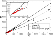
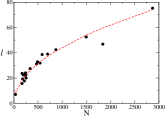
Figure 1: Left: Numbers of roads versus number of nodes (ie. intersections and centers) for data from Cardillo1 (circles) and from Buhl (squares). In the inset, we show a zoom for a small number of nodes. Right: Total length versus the number of nodes. The line is a fit which predicts a growth as $\sqrt{N}$ (data from Cardillo1 ).

These facts are summarized in Fig. 1 (left), together with empirical data from $20$ cities in different continents Cardillo1 . A first important empirical observation is that $1.05\leq e_{emp}\leq 1.69$ , in a range lying between trees and 2d lattices, and the average degree over all these cities is $\langle k\rangle\approx 2.87$. The strongly peaked degree distribution suggests that a quasi-regular lattice could give a fair account of the road network topology. This suggestion is reinforced if one considers the cumulative length $\ell$ of the roads. With this picture in mind, one would expect that for a given average density $\rho=N/L^{2}$, the typical inter distance between nodes is $\ell_{1}\sim\frac{1}{\sqrt{\rho}}$. The total length is then the number of edges times the typical inter-distance which leads to

$$\ell\sim E\ell_{1}\sim\frac{\langle k\rangle}{2}L\sqrt{N}$$ (1)

This behavior is reproduced in fig. (1b), where a fit of the empirical data in Cardillo1 with a function of the form $aN^{1/2}$ gives $a_{emp}\approx 1.46\pm 0.04$ (a fit with a function of the form $aN^{\tau}$ leads to $a\approx 1.51\pm 0.24$ and $\tau\approx 0.49\pm 0.03$). The value $a_{emp}=1.46$ has to be compared with the average degree over all cities. One finds $2.87/2\approx 1.44$ and considering statistical errors, it is hard to reject the hypothesis of a slightly perturbed lattice as a model for the road network.

The two empirical facts above lend credibility to the simple picture that city streets are described by a quasi-regular lattice with an essentially constant degree (equal to approximately $3$) and constant road length ($\ell_{1}\sim 1/\sqrt{\rho}$). There is however a further empirical fact which forces us to reconsider this simple picture. The roads’ network define a tessellations of the surface and the authors of Lammer measured the distribution of the area $A$ of the polygons delimited by the edges of the network. Surprisingly, they found a power law behavior of the form

$$P(A)\sim A^{-\alpha}$$ (2)

with $\alpha\simeq 1.9$ (the standard error is not available in Lammer ). This fact contradicts the simple model of an almost regular lattice since the latter would predict a distribution $P(A)$ very peaked around a value of the order of $\ell_{1}^{2}$. The authors of  Lammer also measured the distribution of the form factor given by the area of a cell divided by the area of the circumscribed circle (for this value they use the largest distance $D$ between nodes of the cell, a convention that we adopted): $\phi=4A/(\pi D^{2})$. They found that most cells have a form factor between $0.3$ and $0.6$ indicating a large variety of cell shapes.

A first challenge is therefore to design a model for planar networks that can reproduce quantitatively these featurees and which is based on a plausible (small) set of assumptions. The simple indicators discussed above show that one cannot model the network by either lattices, Voronoi tessellation, random planar Erdos-Renyi graphs, all these networks having a peaked distribution of areas and form factors. Let’s note that the scale-invariant distribution for cell sizes can be obviously reproduced by assuming by the fractal model of  Kalapala:2006 which assumes a self-similar process of road generation. The power law distribution for cell sizes automatically follows from this assumption. In the following, we present a model that relies on a simple plausible mechanism, does not assume self-similarity and quantitatively accounts for the empirical facts presented above.

III The model of road formation

We first discuss the part of our model that describes the evolution of the road network. Our main assumption is that the network grows by trying to connect to a set of points -the ‘centers’- in an efficient and economic way. These centers can represent either homes, offices or businesses. This parameter free model is based on a principle of local optimality and has been proposed in Barthelemy:2007 . For the sake of self-consistency and readability, we first describe this model in detail. The application of optimality principles to both natural and artificial transportation networks has a long tradition Stevens ; Ball . The rationale to invoke a local optimality principle in this context is that every new road is built to connect a new location to the existing road network in the most efficient way Bejan . During the evolution of the street network, the rule is implemented locally in time and space. This means that at each time step the road network is grown by looking only at the current existing neighboring sites. This reflects the fact that evolution histories greatly exceed the time-horizon of planners. The self-organized pattern of streets emerges as a consequence of the interplay of the geometrical disorder and the local rules of optimality. In this regard our model is quite different from approaches to transportation networks where an equilibrium situation is assumed and which are based on either (i) minimization of an average quantity (e.g. the total travel time), or (ii) on the inclusion of many different socio-economical factors ( e.g. land use).

III.1 Network growth

When new centers (such as new homes or businesses) appear, they need to connect to the existing road network. If at a given stage of the evolution a single new center is present, it is reasonable to assume that it will connect to the nearest point of the existing road network. When two or more new centers are present (as in Fig. 2) and they want to connect to the same point in the network, we assume that economic considerations impose that a single road - from the chosen network’s point - is built to connect both of them.

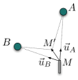
Figure 2: The nearest road to the centers $A$ and $B$ is $M$. The road will grow to point M’. The proposed minimum expenditure principle suggests that the next point M’ will be such that the variation of the total distance to the two points A and B is maximal.

In the example of figure 2, the nearest point of the network to both new centers $A$ and $B$ is $M$. We grow a single new portion of road of fixed length $dx$ from $M$ to a new point $M^{\prime}$ in order to grant the maximum reduction of the cumulative distance of $A$ and $B$ from the network. This translates in the requirement that

$$\delta d=d(M,A)+d(M,B)-[d(M^{\prime},A)+d(M^{\prime},B)]$$ (3)

is maximal ($dx$ being fixed). A simple calculation shows that the maximization of $\delta d$ leads to

$$d\overrightarrow{MM^{\prime}}\propto\vec{u}_{A}+\vec{u}_{B}$$ (4)

where $\vec{u}_{A}$ ($\vec{u}_{B}$) is the unitary vector from $M$ to $A$ ($B$).

The procedure described above is iterated until the road from $M$ reaches the the line connecting $A$ and $B$, where a singularity occurs: $d\overrightarrow{MM^{\prime}}=0$. From there two independent roads to $A$ and $B$ need to be built to connect to the two new centers. The rule Eq. (4) can be easily generalized to the case of $n$ new centers, and, interestingly, was proposed in the context of visualization of leafs’ venation patterns Rolland .

The growth scheme described so far leads to tree-like structures and we implement ideas proposed in Rolland in order to create networks with loops. Indeed, even if tree-like structures are economical, they are hardly efficient: the length of the path along a minimum spanning tree network for example, scales as a power $5/4$ of the Euclidean distance between the end-points Duco . Better accessibility is then granted if loops are present. In order to obtain loops, we assume, following Rolland , that a center can affect the growth of more than one single portion of road per time step and can stimulate the growth from any point in the network which is in its relative neighborhood, a notion which has been introduced in Toussaint . In the present context a point $P$ in the network is in the relative neighborhood of a center $C$ if the intersection of the circles of radius $d(P,C)$ and centered in $P$ and $C$, respectively, contains no other centers or point of the network Toussaint . This definition rigorously captures the loosely defined requirement that, for $v$ to belong to the relative neighborhood of $s$, the region between $s$ and $v$ must be empty. At a given time step, a generic center $C$ then stimulates the addition of new portions of road (pointing to P) from all points in the network that are in its relative neighborood, naturally creating loops. When more than one center stimulates the same point P the prescription of (4) is applied and the evolution ends when the list of stimulated points is exhausted (We refer the interested reader to Barthelemy:2007 for a detailed exposition of the algorithm).

The formula above can be straigthforwardly extended to the case of centers with non-uniform weight $\eta$. This leads to a modified version of Eq. (4), where the sum of distances to be minimized is weighted by $\eta$ and leads to

$$d\overrightarrow{MM^{\prime}}\propto\eta_{A}\vec{u}_{A}+\eta_{B}\vec{u}_{B}.$$ (5)

where $\eta_{A}$ and $\eta_{B}$ can be different. Simulations with non-uniform centers weights show that - as far as the location of ‘heavy’ and ‘light’ centers is uniformly distributed in space, uncorrelated and not broad - that the structure of the network is locally modified, but that its large scale properties are virtually unchanged. In the algorithm presented above, once a center is reached by all the roads it stimulates, it becomes inactive. An interesting variant of this model assumes that centers can stay active indefinetively. In this case we expect a larger effect of the weights’ heterogeneity. We will leave this problem for future studies.

In the following, we study networks resulting from the growth process described above. We assume that the appearance of new centers is given exogenously and is independent from the existing road network and from the position and number of the centers already present. The model accounts quantitatively for a list of descriptors -the ones discussed above in an empirical context- that characterize at a coarse grained level the topology of street patterns. At a more qualitative level, the model leads to the presence of perpendicular intersections, and also reproduces the tendency to have bended roads even if geographical obstacles are absent.

We show in Fig. 3 examples of patterns obtained at different times. The model gives information about the time evolution of the road network: at earlier times, the density is low and the typical inter-distance between centers is large (see Fig. 3). As time passes, the density increases and the typical length to connect a center to the existing road network becomes shorter. Since the number of points grows with time, the simple assumption that the typical road length is given by $1/\sqrt{\rho}$ leads to $\ell_{1}\sim 1/\sqrt{t}$ which is indeed what the model predicts.

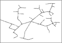
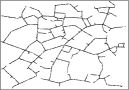
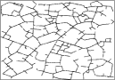
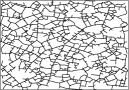
Figure 3: Snapshots of the network at different times of its evolution: for (a) $t=1,000$, (b) $t=2,000$, (c) $t=3,000$, (d) $t=4,000$. At short times, we have a tree structure and loops appear for larger density values obtained at larger times. For $t=4,000$, we have approximately $1,700$ nodes connected by $2,000$ roads.

Beyond visual similarities, the model allows quantitative comparisons with the empirical findings The ratio $e=E/N$, initially close to $1$ (indicating that the corresponding network is tree-like), increases rapidly with $N$, to reach a value of order $1.25$ which is in the ballpark of empirical findings. The cumulative length of the roads produced by the model (Fig. 4a) shows a behavior of the form $a\sqrt{N}$ with $a\approx 1.90$, in good agreement with the empirical measurements $a_{emp}\approx 1.87$). The form factor distribution (Fig. 4b) has an average value $\phi=0.6$ and values essentially contained in the interval $[0.3,0.7]$ in agreement with the results in Lammer for 20 German cities.

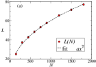
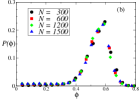
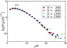
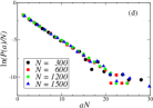
Figure 4: Results of the model (averaged over $1000$ configurations). (a) Total length of roads versus the number of nodes. The dotted line is a square root fit. (b) Structure factor distribution showing a good agreement with the empirical results of Lammer . (c-d) Rescaled distributions of the perimeter (c) and of the areas (d) of the cells displaying an exponential behavior.

III.2 Effect of the center spatial distribution

An important feature of street networks is the large diversity of cell shapes and the broad distribution of cell areas. So far, we have assumed that centers are distributed uniformly across the plane. Within this assumption, the model predicts a cell area distribution following an exponential (with a large cut-off however) as shown in Fig. 4(d) and Fig. 5.

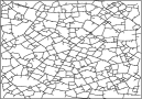
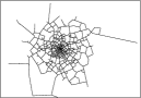
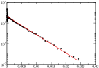
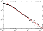
Figure 5: Upper left plot: Uniform distribution of points ($1000$ centers, $100$ configurations). In this case, the area distribution is exponentially distributed (bottom left). Upper right plot: Exponential distribution of centers ($5000$ centers, $100$ configurations, exponential cut-off $r_{c}=0.1$). In this case, we observe a power law (bottom right). The line is a power law fit which gives an exponent $\approx 1.9$.

The empirical distribution of centers in real cities, however, is not accurately described by an uniform distribution but decreases exponentially from the center Makse1 ; Makse2 . We thus use such an exponential distribution $P(r)=\exp(-|r|/r_{c})$ for the center spatial location and measure the areas formed by the resulting network (in the last section of this point is further discussed). Although most quantities (such as the average degree and the total road length) are not very sensitive to the center distribution, the impact on the area distribution is drastic. In Fig. 5 a power law with exponent equal to $1.9\pm 0.1$ is found, in remarkable agreement with the empirical facts reported in Lammer for the city of Dresden. Although we cannot claim that this exponent is the same for all cities, the appearance of a power law in good agreement with empirical observations confirms the fact that the simple local optimization principle is a possible candidate for the main process driving the evolution of city street patterns. This result also demonstrates that the centers’ distribution is crucial in the evolution process of a city.

The optimization process described above has several interesting consequences on the global pattern of the street network when geographical constraints are imposed, as illustrated by the following example. We simulated the presence of a river assuming that new centers cannot appear on a stripe of given width (and are otherwise uniformly distributed).

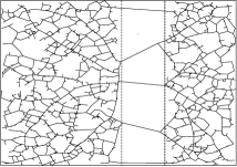
Figure 6: In the presence of an obstacle (here a ‘river’ delimited by the two dotted line) in which the centers are not allowed to be located, the local optimization principle leads to a natural solution with a small number of bridges.

The resulting pattern is shown in Fig. 6. The local optimization principle naturally creates a small number of bridges that are roughly equally spaced along the river and organizes the road network. To conclude, it is worth noting that in the present framework we didn’t attempt the modelization of planning efforts. Simulations show that, at the present simplified stage, the presence of a skeleton of “planned” large roads has the effect of partitioning the plane in different regions where the growth of the network is dominated by the mechanism described above, and reproducing on a smaller scale the structures shown in fig. 3.

III.3 Hierarchical structure of the traffic

Finally, we discuss now the presence of hierarchy in the network generated by the model. Indeed, geographers have recognized for a long time (see e.g. Christaller ) that many systems are organized in a hierarchical fashion. Highways are connected to intermediate roads which in turn dispatch the traffic through smaller roads at smaller spatial scales. In order to test for the existence of such a hierarchy in our model, we use the edge betweenness centrality as a simple proxy for the traffic on the road network. For a generic graph, the betweenness centrality $g(e)$ of an edge $e$ Freeman ; Goh:2001 ; Barthelemy:2003 is the fraction of shortest paths between any pair of nodes in the network that go through $e$. Allowing the possibility of multiple shortest paths between two points, one has

$$g(e)=\sum_{s\neq t}\frac{\sigma_{st}(e)}{\sigma_{st}}$$ (6)

where $\sigma_{st}$ is the number of shortest paths going from $s$ to $t$ and $\sigma_{st}(e)$ is the number of shortest paths going from $s$ to $t$ and passing through $e$. Central edges are therefore those that are most frequently visited if shortest paths are chosen to move from and to arbitrary points.

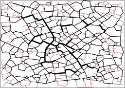
Figure 7: Traffic map of the network. The edge centrality is computed and divided in three different groups and the thickness of the edge is plotted according to the group (from thin to thick for increasing edge centrality.

We computed this quantity for all edges of the road network generated by our algorithm. It appears that this quantity $g(e)$ is broadly distributed and varies over more than $6$ orders of magnitude. In order to get a simple representation of this quantity we arbitrarily group the edges in three classes: $[1,10^{4}]$, $[10^{4},10^{5}]$, $[10^{5},\infty]$ and plot them with different thicknesses. In particular, we see in Fig 7, that edges with the largest centrality (represented by the thickest line) form almost a tree of large arteries. Proportionality between traffic and edge-centrality, as defined above, is virtually equivalent to assuming: i) a uniform origin-destination matrix, ii) everybody choose the shortest path to reach a destination, and iii) roads are “large” enough to support the traffic generated by i) and ii) without congestion effects. Under these assumption one indeed observes a hierarchy of smaller roads and streets with a decreasing typical length and the existence of a hierarchical structure of arteries, roads and streets.

IV Location of centers: effect of density and accessibility

In the simple version of the model presented above, the location of centers are independent from the topology of the road network. In real urban systems, this is however unlikely to happen. There is an extensive spatial economics literature (see Fujita and references therein) that focuses on the several factors that may potentially influence the choice location for new businesses, homes, factories, or offices (see also Jensen and references therein). Empirical evidences suggest a strong correlation between transportation networks and density increase have been recently provided by Levinson Levinson2 . Our goal here is to discuss, based on very simple and plausible assumptions, the coupled evolution of the road network and the population density.

We first divide the city in square sectors of area $S$, and we assume that the choice of a location for a new center is governed by a probability $P(i)$ that one ($i$) of these sectors is chosen. This probability, which reflects the attractiveness of a location, depends a priori on a large number of factors such as accessibility, renting prices, income distribution, number and quality of schools, shops, etc. A key observation made by previous authors (see for example  Brueckner and references therein) is that commuting cost differences must be balanced by differences in living spaces prices. We will follow this observation and we will thus focus on two factors which are the rent price and the accessibility (which we will reduce to commuting costs).

IV.1 Rent price and accessibility

The housing price of a given location is probably determined by many factors comprising tax policies, demography, etc., and is by itself an important subject of study (see for example Goodman ). We will make here the simplifying assumption that the rent price is an increasing function of the local density (for each grid sector) $\rho(i)=N(i)/S$, where $N(i)$ is the number of centers in the sector $(i)$, and in particular that the rent price $C_{R}$ is directly proportional to the local density of population (which can be seen as the first term of an expansion of the price as a function of the density)

$$C_{R}(i)=A\rho(i)$$ (7)

where $A$ is some positive prefactor corresponding to the price per density. We note here that a more general form of the type $C_{R}=A\rho(i)^{\tau}$ could be used. A preliminary study suggests that as long as the rent cost is an increasing function of the density, our results remain qualitatively unchanged. It would be however very interesting to measure this function empirically.

The second important factor for the choice of a location is its accessibility. Locations which are easily accessible and which allow to reach easily arbitrary destinations are more attractive, all other parameters being equal. Also, for a new commercial activity, high traffic areas can strongly enhance profit opportunities. In terms of the existing network, the best locations are therefore the most central and standard models of city formation (see for example Fujita ) indeed integrate the distance to the center and its associated (commuting) cost as a main factor. Euclidean distance, however, can be a poor estimator of the effective accessibility of a given location, if this location is poorly connected to the transportation network. This is why the notion of centrality has to be considered not only in geographical terms, but also from the point of view of the network that grants mobility. The possibility to easily reach an arbitrary location when movement is constrained by a network is nicely captured in quantitative terms by the notion of node betweenness centrality.

In the previous section, we defined the edge betweenness centrality and here we need a similar quantity defined for nodes rather than for edges. The node betweenness centrality $g(v)$ Freeman ; Goh:2001 ; Barthelemy:2003 of a node $v$ is defined as the fraction of shortest paths between any pair of points in the network that go through $v$. The mathematical expression of this quantity is then

$$g(v)=\frac{1}{N(N-1)}\sum_{s\neq t}\frac{\sigma_{st}(v)}{\sigma_{st}}$$ (8)

where $\sigma_{st}$ is the number of shortest paths going from $s$ to $t$ and $\sigma_{st}(v)$ is the number of shortest paths going from $s$ to $t$ and passing through $v$. Betweenness centrality was initially introduced as a natural substitute for geometric centrality in graphs that are not embedded in Euclidean space (see fig. 8).

Figure 8: Illustration of the notion of node betweenness centrality for a non planar graph

Betweenness also naturally serves our purpose to quantify accessibility on planar graphs, especially in our simplified framework where an explicit distinction between resources and users has been sacrified to the sake of simplicity. It is important to note that betweenness centrality, on planar graphs, is strictly correlated to other, more common, measures of centrality. The two first panels of fig 9 show the contour and the 3D plot of node-betweeness for a Manhattan-like grid of 25 blocks per side and clearly show how central nodes are those that are the most frequently visited if shortest paths are chosen to move from and to arbitrary points. The third panel of the same figure shows the relation between the betweenness of a node and its average distance from all other nodes (along the same square grid). This plot demonstrates that the larger the betweenness of a node is, the shorter is its average distance from a generic node.

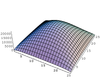
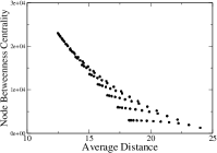
Figure 9: Top panel: Contour plot of node betweenness centrality -not normalized-for a square grid of linear size 25 (A light color indicates a high value of the betweenness). Middle panel: 3D plot of node betweenness centrality (not normalized) for the same square grid. Bottom panel: Plot of the node betweenness of a generic node vs its average distance from all the other nodes.

The betweenness thus extends the concept of geographical centrality to networks whose structure is not a lattice or planar.

In our simple model, we will assume that accessibility reduces here to the facility of reaching quickly any other location in the network. This can also be seen as the average commuting cost which in previous models Fujita was assumed to be proportional to the distance to the center. The natural extension for a network is then to take the transportation cost depending on the betweenness centrality. For each sector $S_{i}$ of the grid, we first compute the average betweenness centrality as

$$\overline{g}(i)=\frac{1}{N(i)}\sum_{v\in S_{i}}g(v).$$ (9)

where the bar represents the average over all nodes (centers and intersections) which belong in a given sector.

Transportation costs are a decreasing function of the betweenness centrality and we will assume here that the transportation cost $C_{T}(i)$ for a center in sector $(i)$ is given by

$$C_{T}(i)=B(g_{m}-\overline{g}(i))$$ (10)

where $B$ and $g_{m}$ are positive constants (other choices, as long as the cost decreases with centrality, linearly or not, give similar qualitative results).

Finally, we will assume (as it is frequently done in many models, see for example Brueckner and references therein) that all new centers have the same income $Y(c)=Y$. This assumption is certainly a rough approximation, as demonstrated by effects such as urban segregation, but in order to not overburden our model, we will neglect income disparities in the present study. The net income of a new center $c$ in a sector $(i)$ is then

$$K(i)=Y-C_{R}(i)-C_{T}(i).$$ (11)

The higher the net income $K(i)$ and the more likely the location $(i)$ will be chosen for the implantation of a new business, home, etc. In urban economics the location is usually chosen by minimizing costs, and we relax this assumption by defining the probability that a new center will choose the sector $(i)$ as its new location under the form

$$P(i)=\frac{e^{\beta K(i)}}{\sum_{j}e^{\beta K(j)}}.$$ (12)

This expression rewritten as

$$P(i)=\frac{e^{\beta(\lambda\overline{g}(i)-\rho(i))}}{\sum_{j}e^{\beta(\lambda\overline{g}(j)-\rho(j))}}$$ (13)

where $\beta A$ is redefined as $\beta$ and where $\lambda=B/A$. For numerical simulations, the local density is normalized by the global density $N/L^{2}$, in order to have the density and centrality contributions defined in the same interval $[0,1]$. The relative weight between centrality and density is then described by $\lambda$ and the parameter $\beta$ implicitly describes in an ‘effective’ way all the factors (which could include anything from individual taste to the presence of schools, malls, etc) that have not been explicitly taken into account, and that may potentially influence the choice of location. If $\beta\approx 0$, cost is irrelevant and new centers will appear uniformly distributed across the different sectors:

$$P(i)\sim\frac{1}{N(i)}.$$ (14)

In the opposite case, $\beta\rightarrow\infty$, the location with the minimal cost will be chosen deterministically.

$$\begin{cases}P(i)=1&\text{for $i$ such that $K(i)$ is minimum}\\ P(i)=0&\text{for all other sectors}\end{cases}$$ (15)

The parameter $\beta$ can thus be used in order to adjust the importance of the cost relative to that of other factors not explicitly included in the model.

V Co-evolution of the network and the density

We finally have all the ingredients needed to simulate the simultaneous evolution of the population density and the road network. Before introducing the full model, analogously to what we have done for the first part of the model, it is worth to study this second part separately. To do that, we consider a toy -one dimensional- case, where the network plays no role, since a single path only exists between each pair of nodes. Despite the simplicity of the setting, it is possible to draw some general conclusion.

V.1 One-dimensional model

We assume that the centers are located on a one-dimensional segment $[-L,L]$. Since only a single path exists between any two points, the calculation of centrality is trivial. In the continuous limit, and for a generic location $x$ it can be written as the product of the number of points that lie at the right and left of the given location

$$g(x)=\int_{-L}^{x}\rho(y,t)dy\left[N-\int_{-L}^{x}\rho(y,t)dy\right]$$ (16)

where $\rho(x,t)$ is the density at $x$. The equation for the density therefore reads:

$$\partial_{t}\rho(x,t)=e^{\beta\left[\lambda\frac{\int_{-L}^{x}\rho(y,t)dy}{N}\frac{(N-\int_{-L}^{x}\rho(y,t)dy)}{N}-\frac{\rho(x,t)}{N}\right]}$$ (17)

where $N=\int_{-L}^{L}\rho(y,t)dy$. The numerical integration of Eq. (17) shows that, after a transient regime, the process locks in a pattern of growth in which the total population grows at a constant rate

$$N=\int_{-L}^{L}\rho(y,t)dy\propto t.$$ (18)

This suggests that a solution for large $t$ can be found via the separation of variables under the form

$$\rho(x,t)=\alpha f(x)t$$ (19)

where one can set $\int_{-L}^{L}f(x)dx=1$ without loss of generality. Plugging the expression (19) into Eq. (17) one gets

$$\alpha f(x)=e^{\beta\left[\lambda\int_{-L}^{x}f(y)dy(1-\int_{-L}^{x}f(y)dy)-f(x)\right]}$$ (20)

where $\alpha$ is an integration constant to be determined. An explicit solution for the inverse $f^{-1}(x)$ can be achieved via the Lambert function (Lambert’s function is the principal branch of the inverse of $z=w\exp^{w}$), but the expression is not particularly illuminating and it is therefore not presented here. Several facts can however be understood using a direct numerical integration of Eq. (17) or the simulation of the relative stochastic process:

• At large times, population in different location grows with a rate $f(x)$ that depends on the location but not explicitely on time. This is a direct consequence of Eq. (19) and is obviously a different behavior from uniform growth. The ratio of population density in two different locations $x_{1}$ and $x_{2}$ stabilizes in the long run to $f(x_{1})/f(x_{2})$

• Although $\beta$ models the ‘noise’ in the choice of location and $\lambda$ the relative importance of centrality as compared to density, they have similar effects on the expected density in a given location. An increase in $\beta$ and $\lambda$ corresponds a concentration of density in the areas of large centrality and a steeper decay of density towards the periphery, as shown in fig. 10a. This can intuitively be understood by looking e.g. at the role played by the parameter $\beta$ in Eq. (10): as $\beta$ decreases to 0, the differences in rate of growth in different locations becomes negligible

• Eq. (17) describes the average (or expected) behavior of the population density over time. Numerical simulations of the corresponding stochastic process show fluctuations from the above mentioned expected value. Such fluctuations increases as noise increases (ie. when $\beta$ decreases).

• Numerical integration of Eq. (17) suggests that, as $\lambda$ increases, the decay of density assumes a power law form whose exponent depends on $\beta$ and $\lambda$ and approaches $-1$ as $\lambda$ gets very large. This can be explained by assuming $f(x)\approx\gamma x^{-r}$, and using Eq. (20) and its derivative both computed in $L$. The derivative of $f(x)$ is:

  $$f^{\prime}(x)=\beta\lambda f(x)\left(1-2\int_{-L}^{x}f(y)dy\right)f(x).$$ (21)

  The above expression can be computed in $x=L$, taking into account that that $\int_{-L}^{L}f(x)dx=1$ and the assumed algebraic functional form of $f(x)$. This leads to

  $$\gamma rL^{-1}=\gamma\beta L^{-r}(\lambda\gamma-r\gamma L^{-1}).$$ (22)

  In the limit of large $L$ one can keep only the leading orders in $L$, and match the power and the coefficient of the leading order on the two sides of the equation above. This gives $r=1$ and $\gamma=1/(\beta\lambda)$. The validity of this argument can be verified looking at fig. 10b, where $\ln(f)$ is plotted vs $\ln(x)$ to highlight the power law behavior of $f(x)$ and where the line $1/(\beta\lambda x)$ has been plotted as a reference for the case $\beta=10$ and $\lambda=10$.

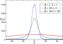
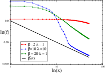
Figure 10: The stationary growth rate for different values of the parameters.(a) Large values of $\beta$ and $\lambda$ implies larger degree of centralization and a faster decay of density from center to periphery. (b) At large values of $\lambda$ the decay of density becomes algebraic for location away from the center. The exponent approaches $-1$ and $f(x)$ is approximated in that region by $1/(\beta\lambda/x)$.

This simple one-dimensional model thus allowed us to understand some basic features of the model that will be discussed in their full generality in the next section.

V.2 Two-dimensional case: existence of a localized regime

We now apply the probability in Eq. (13) to the growth model described in the first part of this paper. The process starts with a ‘seed’ population settlement (few centers distributed over a small area) and a small network of roads that connects them. At any stage, the density and the betweenness centrality of all different subareas are computed, and a few new centers are introduced. Their location in the existing subareas is determined according to the probability defined in Eq. (13). Roads are then grown until the centers that just entered the scene are connected to the existing network. This process is iterated until the desired number of centers has been introduced and connected. In the two panels of figure 11 we show the emergent pattern of roads that is obtained when $\lambda$ is small and very large, respectively.

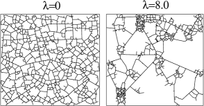
Figure 11: Networks obtained for different values of $\lambda$ (and for $N=500$ and $\beta=1$). On the left, $\lambda=0$ and only the density plays a role and we obtain a uniform distribution of centers. On the right, we show the network obtained for $\lambda=8$. In this case, the centrality is the most important factor leading to a few dominant areas with high density.

When $\lambda$ is small the density plays the dominant role in determining the location of new centers. New centers appear preferably where density is small, smoothing out the eventual fluctuations in density that may occur by chance and the resulting density is uniform. On the other hand, when $\lambda$ is very large, centrality plays the key role, leading to a city where all centers are located in the same small area. The centrality has thus an effect opposite to that of density and tends to favor concentration. We will now describe in more details the transition between the two regimes described above.

We compute, in the two cases, the following quantity (previously introduced in a different context Derrida:1987 ; Barthelemy:2003b ):

$$Y_{2}=\sum_{i}\left[\frac{N(i)}{N}\right]^{2}$$ (23)

where the sum runs over all sectors which number is $N_{s}$. In the uniform case, all the $N(i)$ are approximately equal and one obtains $Y_{2}\sim 1/N_{s}$, which is usually small. In contrast, when most of the population concentrates in just a few sectors which represent a finite fraction of the total population, we obtain $Y_{2}\sim 1/n$ where $n$ represents the order of magnitude of these highly-populated sectors- the ‘dominating sectors’. The quantity

$$\sigma=\frac{1}{Y_{2}N_{s}}$$ (24)

gives therefore the fraction of dominating sectors.

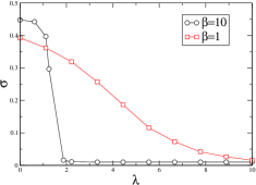
Figure 12: Fraction of dominating sectors (obtained for $500$ centers and averaged over $100$ configurations). When $\lambda$ is small, the center distribution is more uniform and $\sigma$ is large (close to $100\%$).When $\lambda$ increases, we see the appearance of a few sectors dominating and concentrating most of the population. This effect is smoothen out for smaller values of $\beta$ corresponding to the possibility of choice.

The behavior of $\sigma$ vs. $\lambda$ is shown in Fig. 12. We observe that $\sigma$ decreases very fast when $\lambda$ increases, signaling that a phenomenon of localization sets in as soon as transportation costs are involved.

We conclude this section discussing the role played by the parameter $\beta$. Analogously to what happens in the one dimensional case, the concentration effect is weakened by a small values of $\beta$. The parameter $\beta$ describes the overall importance of the cost-factors with respect to other factors that have not been explicitly taken into account, or, equivalently, the possibility of choice. Indeed, when $\beta$ is very large, the location which maximizes the cost is chosen. In contrast, when the parameter $\beta$ is small, the cost differences are smoothen out and a broader range of choices is available for new settlements. Figure 12 illustrates the importance of choice. In particular, the appearance of large-density zones (controlled by the importance of transportation accessibility) is counterbalanced by the possibility of choice and the resulting pattern is more uniform.

V.3 Density profile: the appearance of core districts

In this last part, we describe the effect of the interplay of transportation and rent costs on the decay of population density from the city center. In the following, the core district is identified as the sector with the largest density. The whole plane is then divided in concentric shells with internal radius $r$ and width $dr$. The density profile $\rho(r)$ is given by the ratio of the number $\delta n$ of centers in a shell to its surface $\delta S(r)$

$$\rho(r)=\frac{\delta n}{\delta S}$$ (25)

For small $\lambda$, the density is uniform, as expected. In figure 13 we show the density profile $\rho(r)$ in the case of $\lambda$ large,

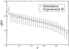
Figure 13: Density profiles for $\lambda=8$ ($N=200$, averaged over $500$ configurations). The decay of the density profile is well fitted by an exponential, signalling the appearance of a well-defined core district (error bars represent one standard deviation).

where we observe a fast exponential decay of the form $\exp{-r/r_{c}}$, in agreement with empirical observations Makse1 . This behavior is the signature of the appearance of a well-defined core district of typical size $r_{c}$, whose typical size $r_{c}$ decreases with $\lambda$. This simplified model predicts, therefore, the existence of a highly populated central area whose size can be estimated in terms of the relative importance of transport and rent costs.

VI Discussion and perspectives

We presented a basic model that describes the impact of economical mechanisms on the evolution of the population density and the topology of the road network. The interplay between rent costs and demand for accessibility leads to a transition in the population spatial density. When transportation costs are moderate, the density is approximately uniform and the road network is a typical planar network that does not show any strong heterogeneity. In contrast, if transportation costs are higher, we observe the appearance of a very densely populated area around which the density decays exponentially, in agreement with previous empirical findings. The model also predicts that the demand for accessibility easily prevails on the disincentive constituted by high rent costs.

A very important ingredient in modeling the evolution of a city is how individuals choose the location for a new business or a new home. We isolated in this work the two important factors of rent price and transportations costs. For these costs, we assume some reasonable forms but it is clear that large scale empirical measures are needed. In particular, it would be interesting to characterize empirically how the rent price varies with the density and how transportation costs varies with the centrality. Possible outcomes to these studies would be to give an idea of the value of the parameter $\lambda$ (and possibly also $\beta$) and thus to determine how much the city is centralized.

As it happens in every modeling effort, a satisfactory compromise between realism and feasibility must be found and we opted for sacrificing some important economic considerations in order to be able to explicitly take into account the topology of the road transportation network and not the distance to a center only, as it is usually assumed in most models. Our model predicts so far the appearance of a core center, but it is however known that cities present a large diversity in their structure, ranging from a monocentric organization to different levels of polycentrism. In addition, interesting scaling relations between different parameters (total wages, walking speed, total traveled length, etc) and population size were recently found  Bettencourt:2007 ; Moses:2007 showing that beyond the apparent diversity, there are some fundamental processes driving the evolution of a city.

These different results appear as various facets of the process of city formation and evolution and it is at this stage not clear how to connect the scaling to the structural organization of a city and more generally, how to reconciliate the different existing results in a unified picture. We believe that the present model- modified or generalized- could help for future studies in this direction.

Acknowledgments. We thank G. Santoboni for many discussions at various stages of this work, and two anonymous referees for several important comments and suggestions. MB also thanks Indiana University for its warm welcome where part of this work was performed.

References

- (1) UN Population division. http://www.unpopulation.org.
- (2) W. Christaller, Central Places in Southern Germany. English translation by C. W. Baskin, London: Prentice hall, (1966).
- (3) D. Levinson and B. Yerra, Transportation Science 40, 179-188 (2006).
- (4) M. Fujita, P. Krugman, A.J. Venables, The Spatial Economy: Cities, Regions, and International Trade, The MIT Press, Cambridge (1999).
- (5) D. Levinson Journal of Economic Geography 8, 55-77, (2008)
- (6) J.H. von Thünen, Von Thünen’s isolated state, Oxford: Pergmanon Press, 1966.
- (7) M. Barthélemy and A. Flammini, Physical Review Letters, 100, 138702 (2008).
- (8) A.K. Dixit and J.E. Stiglitz, Monopolistic competition and optimum product diversity, Amer. Eco. Rev. 67, 297-308 (1977).
- (9) V. Kalapala, V. Sanwalani, A. Clauset, and C Moore Scale invariance in road networks, Phys. Rev. E, 73, 026130 (2006).
- (10) A. Cardillo, S. Scellato, V. Latora S. Porta, Phys. Rev. E 73, 066107 (2006).
- (11) S. Scellato, A. Cardillo, V. Latora, S. Porta, arXiv:physics/0511063.
- (12) J. Buhl, J. Gautrais, N. Reeves, R.V. Sole, S. Valverde, P. Kuntz, G. Theraulaz, Eur. Phys. J. B 49, 513-522 (2006).
- (13) A. Runions, A. M. Fuhrer, B. Lane, P. Federl, A.-G. Rolland-Lagan, and P. Prusinkiewicz, ACM Transactions on Graphics 24(3): 702-711 (2005).
- (14) B. Duplantier, J. Stat. Phys. 54, 581 (1989). A. Coniglio, Phys. Rev. Lett. 62, 3054 (1989).
- (15) G. T. Toussaint, Pattern Recognition, 12, 261 (1980). J. W. Jaromczyk, and G. T. Toussaint, Proc. IEEE, 80, 1502 (1992).
- (16) I. Rodriguez-Iturbe and A. Rinaldo,Fractal river basins: chance and self-organization, Cambridge University Press, Cambridge (1997).
- (17) G. B. West, J. H. Brown, and B. J. Enquist , Science 276, 122, (1997) ;
- (18) M. T. Gastner, and M. E. J. Newman, Phys. Rev. E, 74, 016117, (2006).
- (19) M. Schwartz, Telecommunication networks: protocols, modelling and analysis, Addison-Wesley Longman Publishing Co., Inc. Boston, MA, USA (1986).
- (20) P. S. Stevens, Patterns in Nature, Little, Brown, Boston, (1974).
- (21) P. Ball, The Self-Made Tapestry: Pattern Formation in Nature Oxford University Press, Oxford, (1998).
- (22) G. Doyle and J. L. Snell, Random Walk and Electric Networks, American Mathematical Society, Providence, (1989).
- (23) J. R. Banavar, A. Maritan, and A. Rinaldo, Nature 398, 130 132 (1999).
- (24) A. Maritan, F. Colaiori, A. Flammini, M. Cieplak, and J. R. Banavar, Science 272, 984 986 (1996).
- (25) N. D. Price, J. L. Reed , B. O. Palsson , Nat. Rev. Microbiol. 2, 886 897, (2004).
- (26) J. R. Banavar, F. Colaiori, A. Flammini, A. Maritan, and A. Rinaldo, Phys. Rev. Lett. 84, 4745, (2000).
- (27) R. L. Graham, and P. Hell, Ann. History Comput. 7, 43-57, (1985).
- (28) M.W. Bern and R. L. Graham, Sci. Am. 260, 66 71, (1989).
- (29) R. K. Ahuja, T. L. Magnanti, and J. B. Orlin, Network Flows, Prentice Hall, New Jersey, (1993).
- (30) M. Batty, Cities and Complexity, The MIT press, Cambridge (2005).
- (31) H. A. Makse, S. Havlin, and H. E. Stanley, Nature 377, 608, (2002).
- (32) H. Makse, J.S. Andrade, M. Batty, S. Havlin, H. E. Stanley, Phys. Rev. E 58, 7054 (1998).
- (33) P. Crucitti, V. Latora, S. Porta, Phys. Rev. E 73, 036125 (2006).
- (34) B. Jiang, Env. Plann. B 31, 151-162 (2002).
- (35) S. Lammer, B. Gehlsen, D. Helbing, Physica A 363, 89, (2006).
- (36) S. Porta, P. Crucitti, V. Latora, ArXiv:physics/0506009 (2005).
- (37) M. Roswall, A. Trusina, P. Minnhagen, K. Sneppen, arXiv:cond-mat/0407054.
- (38) B. Jiang, C. Claramunt, Env. Plann. B 31, 151-162 (2004).
- (39) L.A.N. Amaral, A. Scala, M. Barthélemy, H.E. Stanley, Proc. Natl. Acad. Sci. (USA) 97, 11149 (2000).
- (40) C. Itzykson and J.-M. Drouffe, Statistical field theory Vol. 2, Cambridge University Press (1989).
- (41) S. Gerke, C. McDiarmid, Combinatorics, Probability and Computing 13, 165, (2004).
- (42) P. S. Stevens, Patterns in Nature, Little, Brown, Boston, (1974).
- (43) P. Ball, The self-made tapestry: pattern formation in Nature, Oxford University Press,Oxford, (1998).
- (44) A. Bejan and G.A. Ledezma, Physica A 255, 211-217 (1998).
- (45) P. Jensen, Phys. Rev. E (R) 74, 035101 (2006).
- (46) J.K. Brueckner, in E.J. Mills (Ed.) Handbook of regional and urban economics, volume 2, pp. 821-845 (1987).
- (47) A.C. Goodman, Journal of Urban Economics 23, 327-353 (1988).
- (48) L. C. Freeman, Sociometry 40, 35 (1977) .
- (49) K.-I. Goh, B. Kahng, D. Kim, Phys. Rev. Lett. 87, 278701 (2001).
- (50) M. Barthélemy, Eur. Phys. J. B 38, 163 (2003).
- (51) B. Derrida, H. Flyvbjerg, J. Phys. A: Math. Gen. 20, 5273-5288 (1987).
- (52) M. Barthélemy, B. Gondran, E. Guichard, Physica A 319, 633-642 (2003).
- (53) L.M. Bettencourt, J. Lobo, D. Helbing, C. Kuhnert, and G.B. West, Proc. Natl. Acad. Sci. (USA) 104, 7301-7306 (2007).
- (54) H. Samaniego, and M.E. Moses ”Cities as Organisms: Allometric Scaling as an Optimization Model to Assess Road Networks in the USA,” presented at the Access to Destinations II conference, Minneapolis, August 2007.