Verhulst model with Lévy white noise excitation

Abstract

The transient dynamics of the Verhulst model perturbed by arbitrary non-Gaussian white noise is investigated. Based on the infinitely divisible distribution of the Lévy process we study the nonlinear relaxation of the population density for three cases of white non-Gaussian noise: (i) shot noise, (ii) noise with a probability density of increments expressed in terms of Gamma function, and (iii) Cauchy stable noise. We obtain exact results for the probability distribution of the population density in all cases, and for Cauchy stable noise the exact expression of the nonlinear relaxation time is derived. Moreover starting from an initial delta function distribution, we find a transition induced by the multiplicative Lévy noise, from a trimodal probability distribution to a bimodal probability distribution in asymptotics. Finally we find a nonmonotonic behavior of the nonlinear relaxation time as a function of the Cauchy stable noise intensity.

I Introduction

The nonlinear stochastic systems with noise excitation have attracted extensive attention and the concept of noise-induced transitions has got a wide variety of applications in physics, chemistry, and biology Hor84 . Noise-induced transitions are conventionally defined in terms of changes in the number of extrema in the probability distribution of a system variable and may depend both quantitatively and qualitatively on the character of the noise, i.e. on the properties of stochastic process which describes the noise excitation. The Verhulst model, which is a cornerstone of empirical and theoretical ecology, is one of the classic examples of self-organization in many natural and artificial systems Eig79 . This model, also known as the logistic model, is relevant to a wide range of situations including population dynamics Hor84 ; Mor82 ; Ciu93 ; Mat00 , self-replication of macromolecules Eig71 , spread of viral epidemics Ace06 , cancer cell population Bao03 , biological and biochemical systems Der90 ; Ciu96 , population of photons in a single mode laser McN74 ; Oga83 , autocatalytic chemical reactions Sch72 ; Cha76 ; Gar77 ; Bou82 ; Leu87 , freezing of supercooled liquids Das83 , social sciences Her72 ; Mon78 , etc.

In considering how the population density $x\left(t\right)$ may change with time $t$, Verhulst proposed the following equation

$$\frac{dx}{dt}=rx\left(1-\frac{x}{\Omega}\right).$$ (1)

where there is the Malthus term with the rate constant $r$ and a saturation term with the $\Omega$ factor, which is the upper limit for the population growth due to the availability of the resources.

Really the parameters $r$ and $\Omega$ are not constant. In fact the parameter $r$ changes randomly due to season fluctuations, and the parameter $\Omega$ fluctuates due to the environmental interaction which causes the random availability of resources. As a consequence we have the following stochastic Verhulst equation

$$\frac{dx}{dt}=r\left(t\right)x\left[1-\frac{x}{\Omega\left(t\right)}\right].$$ (2)

In the context of macromolecular self-replication, the model equation (2), with constant $\Omega$ and a white Gaussian noise in $r\left(t\right)$, was numerically studied in Ref. Leu88 and the critical slowing down, i.e. a divergence of the relaxation time at some noise intensity, was found. Later Jackson and co-authors Jac89 investigated the same model, by analog experiment and digital simulations. They analyzed specifically in detail the nonlinear relaxation time defined as Bin73

$$T=\frac{\int\nolimits_{0}^{\infty}\left[\left\langle x\left(t\right)\right\rangle-\left\langle x\left(\infty\right)\right\rangle\right]dt}{x\left(0\right)-\left\langle x\left(\infty\right)\right\rangle}$$ (3)

and did not observe the critical slowing down. They explained this discrepancy by the incorrect approximate truncation of the asymptotic power series for $T$ used in Ref. Leu88 . The stability conditions were derived in Ref. Gol03 . Similar investigations for colored Gaussian noise $r(t)$ were performed in Ref. Man90 , where a monotonic dependence of the relaxation time and the correlation time on the noise intensity was found. The generalization of Eq. (2), to study a Bernoulli-Malthus-Verhulst model driven by a multiplicative colored noise, was analyzed recently in Ref. Cal07 .
The evolution of the mean value in the case of Eq. (2) with constant $r$ and white Gaussian noise excitation $\beta\left(t\right)=r/\Omega\left(t\right)$ was considered in Refs. Ciu93 ; Suz82 ; Suz82a ; Bre82 ; Mak85 ; Mor86 . In Refs. Mak85 ; Mor86 the authors, using perturbation technique, obtained the exact expansion in power series on noise intensity of all the moments and found the long-time decay of $t^{-1/2}$. In Ref. Ciu93 the authors derived the long-time behavior of all the moments of the population density by means of an exact asymptotic expansion of the time averaged process generating function, and found the same asymptotic behavior of $t^{-1/2}$ at the critical point. This very slow relaxation of the moments near the critical point is the phenomenon of critical slowing down.
In the present paper, using the previously obtained results for a generalized Langevin equation with a Lévy noise source Dub05 ; Dub08 , we investigate the transient dynamics of the stochastic Verhulst model with a fluctuating growth rate and a constant value for the saturation population density $\Omega$, that is $\Omega=1$. The exact results for the mean value of the population density and its nonstationary probability distribution for different types of white non-Gaussian excitation $r\left(t\right)$ are obtained. We find the interesting noise-induced transitions for the probability distribution of the population density and the relaxation dynamics of its mean value for Cauchy stable noise. Finally we obtain a nonmonotonic behavior of the nonlinear relaxation time as a function of the Cauchy noise intensity.

II Stochastic Verhulst equation with non-Gaussian fluctuations of growth rate

Let us consider Eq. (2) with a constant saturation value $\Omega=1$, namely

$$\frac{dx}{dt}=r\left(t\right)x\left(1-x\right).$$ (4)

After changing variable $y=\ln[x/(1-x)]$, we obtain

$$y\left(t\right)=y\left(0\right)+\int\nolimits_{0}^{t}r\left(\tau\right)d\tau\,$$

and the exact solution of Eq. (4) is

$$x\left(t\right)=\left(1+\frac{1-x_{0}}{x_{0}}\exp\left\{-\int\nolimits_{0}^{t}r\left(\tau\right)d\tau\right\}\right)^{-1},$$ (5)

where $x_{0}=x\left(0\right)$. Now by substituting in Eq. (5) the following expression for the random rate $r(t)$

$$r\left(t\right)=r+\xi\left(t\right),$$ (6)

where $r>0$ and $\xi\left(t\right)$ is an arbitrary white non-Gaussian noise with zero mean, we can rewrite the solution (5) as

$$x\left(t\right)=\left(1+\frac{1-x_{0}}{x_{0}}e^{-rt-L\left(t\right)}\right)^{-1}.$$ (7)

Here $L\left(t\right)$ denotes the so-called Lévy random process with $L\left(0\right)=0$, and $\xi\left(t\right)=\dot{L}\left(t\right)$. As it was shown in Refs. Dub05 ; Dub08 ; Fel71 , Lévy processes having stationary and statistically independent increments on non-overlapping time intervals belongs to the class of stochastic processes with infinitely divisible distributions. As a consequence, the characteristic function of $L\left(t\right)$ can be represented in the following form (see Eq. (6) in  Dub05 )

$$\left\langle e^{iuL\left(t\right)}\right\rangle=\exp\left\{t\int\nolimits_{-\infty}^{+\infty}\frac{e^{iuz}-1-iu\sin z}{z^{2}}\rho\left(z\right)dz\right\},$$ (8)

where $\rho\left(z\right)$ is some non-negative kernel function. The case $\rho\left(z\right)=2D\delta\left(z\right)$ corresponds to a white Gaussian noise excitation $\xi\left(t\right)$, while for a symmetric Lévy stable noise $\xi\left(t\right)$ with index $\alpha$ we have a power-law kernel $\rho\left(z\right)=Q\left|z\right|^{1-\alpha}$, with $0<\alpha<2$.

In the model under consideration the stationary probability distribution has: (i) a singularity at the stable point $x=1$ for white Gaussian noise, and (ii) two singularities at both stable points $x=0$ and $x=1$ for Lévy noise. To analyze the time behavior of the probability distribution in the transient dynamics it is better not to use the Kolmogorov equation for the probability density $P\left(x,t\right)$, but rather the exact solution (7). Using the standard theorem of the probability theory regarding a nonlinear transformation of a random variable, we find from Eq. (7)

$$P\left(x,t\right)=\frac{1}{x\left(1-x\right)}P_{L}\left(\ln\left[\frac{\left(1-x_{0}\right)x}{x_{0}\left(1-x\right)}\right]-rt,t\right),$$ (9)

where $P_{L}\left(z,t\right)$ is the probability density corresponding to the characteristic function (8). For a white Gaussian noise $\xi\left(t\right)$, this distribution reads

$$P_{L}\left(z,t\right)=\frac{1}{2\sqrt{\pi Dt}}\exp\left\{-\frac{z^{2}}{4Dt}\right\}.$$ (10)

The time evolution of the probability distribution $P\left(x,t\right)$ for $D=0.5$, $r=1$, and $x_{0}=0.2$ is plotted in Fig. 1.

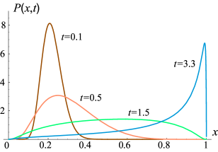
Figure 1: Time evolution of the probability distribution of the population density for white Gaussian noise excitation with intensity $D$. The values of the parameters are: $x_{0}=0.2$, $r=1$, $D=0.5$.

As it is easily seen, the maximum of the unimodal distribution with initial position at $x=0.2$ shifts with time towards the stable point at $x=1$. At the same time, as it follows from Eqs. (9) and (10), for all $t>0$ we have

$$\lim_{x\rightarrow 0^{+}}P\left(x,t\right)=\lim_{x\rightarrow 1^{-}}P\left(x,t\right)=0.$$ (11)

The same picture is observed for another kernel function $\rho\left(z\right)=Kz/\left(2\sinh z\right)$ $\left(K>0\right)$, corresponding to a Lévy process $\eta\left(t\right)$ with finite moments and the following probability density of increments

$$P_{L}\left(z,t\right)=\frac{2^{Kt-1}}{\pi^{2}\Gamma\left(Kt\right)}\Gamma\left(\frac{Kt}{2}+\frac{iz}{\pi}\right)\Gamma\left(\frac{Kt}{2}-\frac{iz}{\pi}\right),$$ (12)

where $\Gamma\left(x\right)$ is the Gamma function. The corresponding time evolution of the probability distribution $P\left(x,t\right)$ for $K=0.43$, $r=1$, and $x_{0}=0.2$ is shown in Fig. 2.

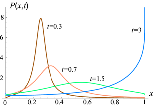
Figure 2: Time evolution of the probability distribution of the population density in the case of Lévy noise with distribution (12). The values of the parameters are: $x_{0}=0.2$, $r=1$, $K=0.43$.

A different situation we have for a Cauchy stable noise $\xi\left(t\right)$ with constant kernel $\rho\left(z\right)=Q$ $\left(\alpha=1\right)$. After evaluation of the integral in Eq. (8), the probability density of the Lévy process increments takes the form of the well-known Cauchy distribution Fel71

$$P_{L}\left(z,t\right)=\frac{D_{1}t}{\pi\left[z^{2}+\left(D_{1}t\right)^{2}\right]},$$ (13)

where $D_{1}=\pi Q$ is the noise intensity parameter. In such a case from Eqs. (9) and (13) for all $t>0$ we find

$$\lim_{x\rightarrow 0^{+}}P\left(x,t\right)=\lim_{x\rightarrow 1^{-}}P\left(x,t\right)=\infty.$$ (14)

As a result, from an initial delta function we immediately obtain a trimodal distribution for $t>0$ and then after some transition time $t_{c}$ a bimodal one with two singularities at the stable points $x=0$ and $x=1$ (see Figs. 3, 4 and 5). We should note that the transition from trimodal to bimodal distribution is a general feature of the model in the presence of a Cauchy stable noise, and it is not limited to some range of parameters. In fact, from Eq. (14) and a delta function initial distribution inside the interval (0,1), this transition always takes place.

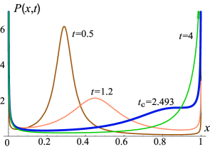
Figure 3: Time evolution of the probability distribution of the population density in the case of white Cauchy noise excitation. The values of the parameters are: $x_{0}=0.2$, $r=1$, $D_{1}=0.5$.

In the following Figs. 4 and 5 we show the time evolution of the probability distribution of the population density for two other values of the noise intensity, namely $D_{1}=1$ and $D_{1}=5$. As the noise intensity increases the probability distribution shows two singularities near $x=0$ and $x=1$ with different amplitude.

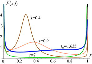
Figure 4: Time evolution of the probability distribution of the population density in the case of white Cauchy noise. The values of the parameters are $x_{0}=0.2$, $r=1$, $D_{1}=1$.

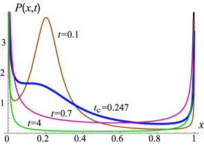
Figure 5: Time evolution of the probability distribution of the population density in the case of white Cauchy noise. The values of the parameters are $x_{0}=0.2$, $r=1$, $D_{1}=5$.

This transition in the shape of the probability distribution of the population density is due to both the multiplicative noise and the Lévy noise source. Using Eqs. (9) and (13) and equating to zero the derivative of $P(x,t)$ with respect to $x$, we obtain the following condition for the extrema in the range $0<x<1$, and particularly for a minimum in the same interval

$$\frac{z(x,t)}{z(x,t)^{2}+(D_{1}t)^{2}}=x-\frac{1}{2}\;,$$ (15)

with

$$z(x,t)=\ln\left[\frac{\left(1-x_{0}\right)x}{x_{0}\left(1-x\right)}\right]-rt\,.$$ (16)

This condition can be solved graphically by finding the intersection between the functions $y_{1}=z(x,t)/(z(x,t)^{2}+(D_{1}t)^{2})$ and $y_{2}=x-1/2$. This is done in the following Figs. 6, 7, 8, where the function $y_{1}$ is plotted for three different values of time and noise intensity. In each figure the black blue curve (color on line) corresponds to the critical value of time $t_{c}$ for which we have a noise induced transition of the probability distribution of the population density from trimodal to bimodal, that is from two minima and one maximum to one minimum inside the interval $0<x<1$. The appearance of one minimum in the probability distribution is the signature of this transition.

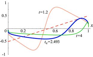
Figure 6: Plots of both sides of Eq. (15) (white Cauchy noise): function $y_{1}$ (solid curves), function $y_{2}$ (dashed curve), for three values of time, namely: $t=1,\,1.5,\,2.493$. The critical time is $t_{c}=2.493$ (black blue curve). The values of the other parameters are: $x_{0}=0.2$, $r=1$, $D_{1}=0.5$.

Figure 7: Plots of both sides of Eq. (15) (white Cauchy noise): function $y_{1}$ (solid curves), function $y_{2}$ (dashed curve), for three values of time, namely: $t=0.5,\,1,\,1.635$. The critical time is $t_{c}=1.635$ (black blue curve). The values of the other parameters are: $x_{0}=0.2$, $r=1$, $D_{1}=1$.

The three values of the critical time $t_{c}$ corresponding to the three values of the Lévy noise intensity investigated are: $D_{1}=0.5,~{}t_{c}=2.493;~{}D_{1}=1,~{}t_{c}=1.635;~{}D_{1}=5,~{}t_{c}=0.247$. One rough evaluation of the critical time $t_{c}$ is obtained by putting equal to $1$ the scale parameter of the Cauchy distribution of Eq. (13), that is $t_{c}\sim 1/D_{1}$. The critical time $t_{c}$ is the time at which the maximum and one minimum of the probability distribution (see Figs. 3, 4, and 5) coalesce in one inflection point and in this point $x$ the function $y_{2}=x-1/2$ becomes tangent at the function $y_{1}$ (see Figs. 6, 7, and 8). It is interesting to note that the critical time $t_{c}$ decreases with the noise intensity $D_{1}$. This is because by increasing the noise intensity, more quickly the population density reaches the two points near the boundaries $x=0$ and $x=1$.

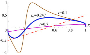
Figure 8: Plots of both sides of Eq. (15) (white Cauchy noise): function $y_{1}$ (solid curves), function $y_{2}$ (dashed curve), for three values of time, namely: $t=0.5,\,1,\,1.635$. The critical time is $t_{c}=0.247$ (black blue curve). The values of the other parameters are: $x_{0}=0.2$, $r=1$, $D_{1}=5$.

III Nonlinear relaxation time of the mean population density

It must be emphasized that to find the time evolution of the mean population density one can use two different approaches. The first one was proposed in Ref. Jac89 . According to the exact solution (7) of the Verhulst equation (4), we can rewrite this expression in the following form

$$x\left(t\right)=f\left(e^{-rt-L\left(t\right)}\right),$$ (17)

where

$$f\left(q\right)=\left(1+\frac{1-x_{0}}{x_{0}}q(t)\right)^{-1}.$$ (18)

Then, by expanding the smooth function (18) in a standard Taylor power series in $q$ around the point $q=0$ we have

$$f\left(q\right)=\sum\limits_{n=0}^{\infty}\frac{f^{\left(n\right)}\left(0\right)}{n!}q^{n}.$$ (19)

After substitution of Eq. (19) in Eq. (17) and averaging we obtain

$$\left\langle x\left(t\right)\right\rangle=\sum\limits_{n=0}^{\infty}\frac{f^{\left(n\right)}\left(0\right)e^{-nrt}}{n!}\left\langle e^{-nL\left(t\right)}\right\rangle$$ (20)

or, in accordance with Eq. (8),

$$\left\langle x\left(t\right)\right\rangle = \sum\limits_{n=0}^{\infty}\frac{f^{\left(n\right)}\left(0\right)e^{-nrt}}{n!}$$

$$\times \exp\left\{t\int_{-\infty}^{+\infty}\frac{e^{-nz}-1+n\sin z}{z^{2}}\,\rho\left(z\right)dz\right\}.$$

For white Gaussian noise $\xi\left(t\right)$ with kernel $\rho\left(z\right)=2D\delta(z)$ we obtain from Eq. (III) the following asymptotic series

$$\left\langle x\left(t\right)\right\rangle=\sum\limits_{n=0}^{\infty}\frac{f^{\left(n\right)}\left(0\right)}{n!}e^{Dtn^{2}-nrt}.$$ (22)

By considering a finite number of terms in this expansion leads to a wrong conclusion about the critical slowing down phenomenon in such a system, as found in Ref. Leu88 . The exact result is obtained, of course, by summing all the terms in Eq. (22). Moreover, for most of the kernels $\rho(z)$ the integral in Eq. (III) diverges. Thus, this approach is inappropriate for our purposes, and it is better to use the direct average in Eq. (7). Therefore, using this second approach we have

$$\left\langle x\left(t\right)\right\rangle=\int\nolimits_{-\infty}^{+\infty}\left(1+\frac{1-x_{0}}{x_{0}}e^{-rt-z}\right)^{-1}P_{L}\left(z,t\right)dz.$$ (23)

Let us consider now different models of white non-Gaussian noise $\xi\left(t\right)$. We start with the white shot noise

$$\xi\left(t\right)=\sum\limits_{i}a_{i}\delta\left(t-t_{i}\right)$$ (24)

having the symmetric dichotomous distribution of the pulse amplitude $P(a)=\left[\delta\left(a-a_{0}\right)+\delta\left(a+a_{0}\right)\right]/2$, mean frequency $\nu$ of pulse train, and kernel $\rho\left(z\right)=\nu z^{2}P\left(z\right)$. From Eq. (8) we have

$$\left\langle e^{iuL\left(t\right)}\right\rangle=e^{-\nu t\left(1-\cos a_{0}u\right)}.$$ (25)

By making the reverse Fourier transform in Eq. (25) we find the probability distribution of the corresponding Lévy process

$$P_{L}\left(z,t\right)=e^{-\nu t}\sum_{n=-\infty}^{+\infty}I_{n}\left(\nu t\right)\delta\left(z-na_{0}\right),$$ (26)

where $I_{n}\left(x\right)$ is the $n$-order modified Bessel function of the first kind. The relaxation of the mean population density $x(t)$ is shown in Fig. 9. According to the Eq. (23) and (26) the stationary value of the population density in such a case is $\left\langle x\right\rangle_{st}=1$, but the relaxation time (3) increases with increasing the mean frequency of pulses.

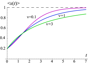
Figure 9: Nonlinear relaxation of the mean population density in the case of white shot noise excitation, for three values of the mean frequency $\nu$, namely $\nu=0.1,1,3$. The values of the other parameters are: $x_{0}=0.2,r=1,a_{0}=1$.

For white non-Gaussian noise with the kernel $\rho(z)=Kz/\left(2\sinh z\right)$ we observe a similar transient dynamics, which is shown in Fig. 10. We have the same stationary value $\left\langle x\right\rangle_{st}$, and the relaxation time $T$ increases with increasing the parameter $K$, which is proportional to the noise intensity.

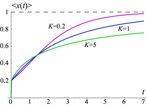
Figure 10: Nonlinear relaxation of the mean population density in the case of Lévy noise with distribution (13), for three values of the parameter $K$, namely $K=0.2,1,5$. The values of the other parameters are: $x_{0}=0.2,r=1$.

Finally, in the case of white Cauchy noise $\xi\left(t\right)$ we obtain interesting exact analytical results. First of all, substituting Eq. (13) in Eq. (23) and changing the variable $z=D_{1}ty$ under the integral, we obtain

$$\left\langle x\left(t\right)\right\rangle=\frac{1}{\pi}\int\nolimits_{-\infty}^{+\infty}\left[1+\frac{1-x_{0}}{x_{0}}e^{-t\left(r+D_{1}y\right)}\right]^{-1}\frac{dy}{1+y^{2}}.$$ (27)

For the stationary mean value $\left\langle x\right\rangle_{st}$ we find from Eq. (27)

$$\left\langle x\right\rangle_{st}=\lim_{t\rightarrow\infty}\left\langle x\left(t\right)\right\rangle=\frac{1}{\pi}\int\nolimits_{-\infty}^{+\infty}\frac{1\left(r+D_{1}y\right)dy}{1+y^{2}},$$ (28)

where $1\left(x\right)$ is the step function. After evaluation of the integral in Eq. (28) we obtain finally

$$\left\langle x\right\rangle_{st}=\frac{1}{2}+\frac{1}{\pi}\arctan\frac{r}{D_{1}}.$$ (29)

As it is seen from Fig. 11 and Eq. (29), for small noise intensity $D_{1}$, with respect to the value of the rate parameter $r=1$, the stationary mean value of the population density is approximately $1$, as for the other white non-Gaussian noise excitations considered. But for large values of $D_{1}$, this asymptotic value, which is independent from the initial value of population density $x_{0}$, tends to $0.5$.

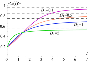
Figure 11: Nonlinear relaxation of the mean population density in the case of white Cauchy noise, for four values of the noise intensity $D_{1}$, namely $D_{1}=0.1,0.5,1,5$. The values of the other parameters are: $x_{0}=0.2,r=1$.

It is interesting also to analyze, for this case of white Cauchy noise, the dependence of the relaxation time $T$ from the noise intensity $D_{1}$. Substituting Eq. (27) in Eq. (3) and changing the order of integration, for initial condition $x_{0}=0.5$, we are able to calculate analytically the double integral in $t$ and in $y$ obtaining the final result

$$T=\frac{\pi\ln 2}{r\left(1+D_{1}^{2}/r^{2}\right)arccot(D_{1}/r)}.$$ (30)

We find a non-monotonic behavior of the relaxation time $T$ versus the noise intensity $D_{1}$ with a maximum at the noise intensity $D_{1}=0.43$, as shown in Fig. 12.

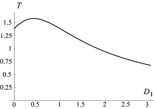
Figure 12: Nonmonotonic behavior of the nonlinear relaxation time $T$ as a function of the white Cauchy noise intensity $D_{1}$. The values of the other parameters are: $x_{0}=0.5,r=1$.

This nonmonotonic behavior is also visible for another initial position $x_{0}=0.2$, as shown in Fig. 11. Here the relaxation time to reach the stationary value of population density $x_{st}$ increases from very low noise intensity ($D_{1}=0.1$) to moderate low intensity ($D_{1}=0.5$), while decreases for higher noise intensities ($D_{1}=1.5$). This is also due to the dependence of $x_{st}$ from the noise intensity $D_{1}$ (see Eq. (30)). We note that this non-monotonic behavior of the relaxation time $T$ is related to the peculiarities of the transient dynamics of the mean population density and it will be object of further investigations.

IV Conclusions

The transient dynamics of the Verhulst model, perturbed by arbitrary non-Gaussian white noise, is investigated. This well-known equation is an appropriate ecological and biological model to describe closed-population dynamics, self-replication of  macromolecules under constraint, cancer growth, spread of viral epidemics, etc… By using the properties of the infinitely divisible distribution of the generalized Wiener process, we analyzed the effect of different non-Gaussian white sources on the nonlinear relaxation of the mean population density and on the time evolution of the probability distribution of the population density. We obtain exact results for the nonstationary probability distribution in all cases investigated and for the Cauchy stable noise we derive the exact analytical expression of the nonlinear relaxation time. Due to the presence of a Lévy multiplicative noise, the probability distribution of the population density exhibits a transition from a trimodal to a bimodal distribution in asymptotics. This transition, characterized by the appearance of a minimum, happens at a critical time $t_{c}$, which can be roughly evaluated as $t_{c}\sim 1/D_{1}$ (where $D_{1}$ is the noise intensity) and exactly evaluated from the condition (15). Finally a nonmonotonic behavior of the nonlinear relaxation time of the population density as a function of the Cauchy noise intensity was found.

References

- (1) W. Horsthemke and R. Lefever, Noise-Induced Transitions: Theory and Applications in Physics, Chemistry and Biology, (Springer–Verlag, Berlin, 1984).
- (2) M. Eigen and P. Schuster, The Hypercycle: A Principle of Natural Self-Organization, (Springer, Berlin, 1979).
- (3) A. Morita, J. Chem. Phys. 76, (1982) 4191–4194.
- (4) S. Ciuchi, F. de Pasquale, and B. Spagnolo, Phys. Rev. E 47, (1993) 3915–3926.
- (5) J. H. Mathis and T. R. Kiffe, Stochastic Population Models: A Compartmental Perspective, (Springer–Verlag, Berlin, 1984).
- (6) M. Eigen, Naturwissenschaften 58, (1971) 465–523.
- (7) L. Acedo, Physica A 370, (2006) 613–624.
- (8) Bao-Quan Ai, Xian-Ju Wang, Guo-Tao Liu, and Liang-Gang Liu, Phys. Rev. E 67, (2003) 022903-1–022903-3.
- (9) G. DeRise and J. A. Adam, J. Phys. A: Math. Gen. 23, (1990) L727S–L731S.
- (10) S. Ciuchi, F. de Pasquale, and B. Spagnolo, Phys. Rev. E 54, (1996) 706–716.
- (11) K. J. McNeil and D. F. Walls, J. Stat. Phys. 10, (1974) 439–448.
- (12) H. Ogata, Phys. Rev. A 28, (1983) 2296–2299.
- (13) F. Schlgl, Z. Phys. 253, (1972) 147–161.
- (14) S. Chaturvedi, C. W. Gardiner, and D. F. Walls, Phys. Lett. A 57, (1976) 404–406.
- (15) C. W. Gardiner and S. Chaturvedi, J. Stat. Phys. 17, (1977) 429–468.
- (16) V. Bouch, J. Phys. A: Math. Gen. 15, (1982) 1841–1848.
- (17) H. K. Leung, J. Chem. Phys. 86, (1987) 6847–6851.
- (18) A. K. Das, Can. J. Phys. 61, (1983) 1046–1049.
- (19) R. Herman and E. W. Montroll, Proc. Natl. Acad. Sci. U.S.A. 69, (1972) 3019–3023.
- (20) E. W. Montroll, Proc. Natl. Acad. Sci. U.S.A. 75, (1978) 4633–4637.
- (21) H. K. Leung, Phys. Rev. A 37, (1988) 1341–1344.
- (22) P. J. Jackson, C. J. Lambert, R. Mannella, P. Martano, P. V. E. McClintock, and N. G. Stocks, Phys. Rev. A 40, (1989) 2875–2878.
- (23) K. Binder, Phys. Rev. B 8, (1973) 3423–3436.
- (24) J. Golec and S. Sathananthan, Math. Comput. Modell. 38, (2003) 585–593.
- (25) R. Mannella, C. J. Lambert, N. G. Stocks, and P. V. E. McClintock, Phys. Rev. A 41, (1990) 3016–3020.
- (26) H. Calisto and M. Bologna, Phys. Rev. E 75, (2007) 050103-1–050103-4(R).
- (27) M. Suzuki, K. Kaneko, and S. Takesue, Prog. Theor. Phys. 67, (1982) 1756–1775.
- (28) M. Suzuki, S. Takesue, and F. Sasagawa, Prog. Theor. Phys. 68, (1982) 98–115.
- (29) L. Brenig and N. Banai, Physica D 5, (1982) 208–226.
- (30) J. Makino and A. Morita, Progr. Theor. Phys. 73, (1985) 1268–1267.
- (31) A. Morita and J. Makino, Phys. Rev. A 34, (1986) 1595–1598.
- (32) A. A. Dubkov and B. Spagnolo, Fluct. Noise Lett. 5, (2005) L267–L274.
- (33) Alexander A. Dubkov, Bernardo Spagnolo, and Vladimir V. Uchaikin, ”Lévy flights Superdiffusion: An Introduction”, Intern. Journ. of Bifurcation and Chaos (2008), in press.
- (34) W. Feller, An Introduction to Probability Theory and its Applications, Vol. 2 (John Wiley & Sons, Inc., New York 1971).