Community Structure in Large Networks: Natural Cluster Sizes and the Absence of Large Well-Defined Clusters

Abstract

A large body of work has been devoted to defining and identifying clusters or communities in social and information networks, i.e., in graphs in which the nodes represent underlying social entities and the edges represent some sort of interaction between pairs of nodes. Most such research begins with the premise that a community or a cluster should be thought of as a set of nodes that has more and/or better connections between its members than to the remainder of the network. In this paper, we explore from a novel perspective several questions related to identifying meaningful communities in large social and information networks, and we come to several striking conclusions.

Rather than defining a procedure to extract sets of nodes from a graph and then attempt to interpret these sets as a “real” communities, we employ approximation algorithms for the graph partitioning problem to characterize as a function of size the statistical and structural properties of partitions of graphs that could plausibly be interpreted as communities. In particular, we define the network community profile plot, which characterizes the “best” possible community—according to the conductance measure—over a wide range of size scales. We study over $100$ large real-world networks, ranging from traditional and on-line social networks, to technological and information networks and web graphs, and ranging in size from thousands up to tens of millions of nodes.

Our results suggest a significantly more refined picture of community structure in large networks than has been appreciated previously. Our observations agree with previous work on small networks, but we show that large networks have a very different structure. In particular, we observe tight communities that are barely connected to the rest of the network at very small size scales (up to $\approx 100$ nodes); and communities of size scale beyond $\approx 100$ nodes gradually “blend into” the expander-like core of the network and thus become less “community-like,” with a roughly inverse relationship between community size and optimal community quality. This observation agrees well with the so-called Dunbar number which gives a limit to the size of a well-functioning community.

However, this behavior is not explained, even at a qualitative level, by any of the commonly-used network generation models. Moreover, it is exactly the opposite of what one would expect based on intuition from expander graphs, low-dimensional or manifold-like graphs, and from small social networks that have served as testbeds of community detection algorithms. The relatively gradual increase of the network community profile plot as a function of increasing community size depends in a subtle manner on the way in which local clustering information is propagated from smaller to larger size scales in the network. We have found that a generative graph model, in which new edges are added via an iterative “forest fire” burning process, is able to produce graphs exhibiting a network community profile plot similar to what we observe in our network datasets.

 

 

1 Introduction

A large amount of research has been devoted to the task of defining and identifying communities in social and information networks, i.e., in graphs in which the nodes represent underlying social entities and the edges represent interactions between pairs of nodes. Most recent papers on the subject of community detection in large networks begin by noting that it is a matter of common experience that communities exist in such networks. These papers then note that, although there is no agreed-upon definition for a community, a community should be thought of as a set of nodes that has more and/or better connections between its members than between its members and the remainder of the network. These papers then apply a range of algorithmic techniques and intuitions to extract subsets of nodes and then interpret these subsets as meaningful communities corresponding to some underlying “true” real-world communities. In this paper, we explore from a novel perspective several questions related to identifying meaningful communities in large sparse networks, and we come to several striking conclusions that have implications for community detection and graph partitioning in such networks. We emphasize that, in contrast to most of the previous work on this subject, we look at very large networks of up to millions of nodes, and we observe very different phenomena than is seen in small commonly-analyzed networks.

1.1 Overview of our approach

At the risk of oversimplifying the large and often intricate body of work on community detection in complex networks, the following five-part story describes the general methodology:

1. Data are modeled by an “interaction graph.” In particular, part of the world gets mapped to a graph in which nodes represent entities and edges represent some type of interaction between pairs of those entities. For example, in a social network, nodes may represent individual people and edges may represent friendships, interactions or communication between pairs of those people.

2. The hypothesis is made that the world contains groups of entities that interact more strongly amongst themselves than with the outside world, and hence the interaction graph should contain sets of nodes, i.e., communities, that have more and/or better-connected “internal edges” connecting members of the set than “cut edges” connecting the set to the rest of the world.

3. A objective function or metric is chosen to formalize this idea of groups with more intra-group than inter-group connectivity.

4. An algorithm is then selected to find sets of nodes that exactly or approximately optimize this or some other related metric. Sets of nodes that the algorithm finds are then called “clusters,” “communities,” “groups,” “classes,” or “modules”.

5. The clusters or communities or modules are evaluated in some way. For example, one may map the sets of nodes back to the real world to see whether they appear to make intuitive sense as a plausible “real” community. Alternatively, one may attempt to acquire some form of “ground truth,” in which case the set of nodes output by the algorithm may be compared with it.

With respect to points (1)–(4), we follow the usual path. In particular, we adopt points (1) and (2), and we then explore the consequence of making such a choice, i.e., of making such an hypothesis and modeling assumption. For point (3), we choose a natural and widely-adopted notion of community goodness (community quality score) called conductance, which is also known as the normalized cut metric [34, 147, 93]. Informally, the conductance of a set of nodes (defined and discussed in more detail in Section 2.3) is the ratio of the number of “cut” edges between that set and its complement divided by the number of “internal” edges inside that set. Thus, to be a good community, a set of nodes should have small conductance, i.e., it should have many internal edges and few edges pointing to the rest of the network. Conductance is widely used to capture the intuition of a good community; it is a fundamental combinatorial quantity; and it has a very natural interpretation in terms of random walks on the interaction graph. Moreover, since there exist a rich suite of both theoretical and practical algorithms [87, 149, 107, 108, 17, 95, 96, 162, 54], we can for point (4) compare and contrast several methods to approximately optimize it. To illustrate conductance, note that of the three $5$-node sets $A$, $B$, and $C$ illustrated in the graph in Figure 1, $B$ has the best (the lowest) conductance and is thus the most community-like.

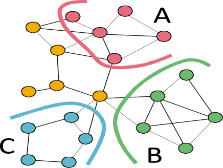
Figure 1: Network communities. Of the three $5$-nodes sets that have been marked, $B$ has the best (i.e., the lowest) conductance, as it has the lowest ratio between the number of edges cut and the number of edges inside. So, set $B$ is the best $5$-node community or the most community-like set of $5$ nodes in this particular network.

However, it is in point (5) that we deviate from previous work. Instead of focusing on individual groups of nodes and trying to interpret them as “real” communities, we investigate statistical properties of a large number of communities over a wide range of size scales in over $100$ large sparse real-world social and information networks. We take a step back and ask questions such as: How well do real graphs split into communities? What is a good way to measure and characterize presence or absence of community structure in networks? What are typical community sizes and typical community qualities?

To address these and related questions, we introduce the concept of a network community profile (NCP) plot that we define and describe in more detail in Section 3.1. Intuitively, the network community profile plot measures the score of “best” community as a function of community size in a network. Formally, we define it as the conductance value of the minimum conductance set of cardinality $k$ in the network, as a function of $k$. As defined, the NCP plot will be NP-hard to compute exactly, so operationally we will use several natural approximation algorithms for solving the Minimum Conductance Cut Problem in order to compute different approximations to it. By comparing and contrasting these plots for a large number of networks, and by computing other related structural properties, we obtain results that suggest a significantly more refined picture of the community structure in large real-world networks than has been appreciated previously.

We have gone to a great deal of effort to be confident that we are computing quantities fundamental to the networks we are considering, rather than artifacts of the approximation algorithms we employ. In particular:

• We use several classes of graph partitioning algorithms to probe the networks for sets of nodes that could plausibly be interpreted as communities. These algorithms, including flow-based methods, spectral methods, and hierarchical methods, have complementary strengths and weaknesses that are well understood both in theory and in practice. For example, flow-based methods are known to have difficulties with expanders [107, 108], and flow-based post-processing of other methods are known in practice to yield cuts with extremely good conductance values [104, 106]. On the other hand, spectral methods are known to have difficulties when they confuse long paths with deep cuts [149, 84], a consequence of which is that they may be viewed as computing a “regularized” approximation to the network community profile plot. (See Section 5 for a more detailed discussion of these and related issues.)

• We compute spectral-based lower bounds and also semidefinite-programming-based lower bounds for the conductance of our network datasets.

• We compute a wide range of other structural properties of the networks, e.g., sizes, degree distributions, maximum and average diameters of the purported communities, internal versus external conductance values of the purported communities, etc.

• We recompute statistics on versions of the networks that have been modified in well-understood ways, e.g., by removing small barely-connected sets of nodes or by randomizing the edges.

• We compare our results across not only over $100$ large social and information networks, but also numerous commonly-studied small social networks, expanders, and low-dimensional manifold-like objects, and we compare our results on each network with what is known from the field from which the network is drawn. To our knowledge, this makes ours the most extensive such analysis of the community structure in large real-world social and information networks.

• We compare results with analytical and/or simulational results on a wide range of commonly and not-so-commonly used network generation models [127, 25, 9, 102, 138, 112, 71, 72].

1.2 Summary of our results

Main Empirical Findings: Taken as a whole, the results we present in this paper suggest a rather detailed and somewhat counterintuitive picture of the community structure in large social and information networks. Several qualitative properties of community structure, as revealed by the network community profile plot, are nearly universal:

• Up to a size scale, which empirically is roughly $100$ nodes, there not only exist cuts with relatively good conductance, i.e., good communities, but also the slope of the network community profile plot is generally sloping downward. This latter point suggests that smaller communities can be combined into meaningful larger communities, a phenomenon that we empirically observe in many cases.

• At the size scale of roughly $100$ nodes, we often observe the global minimum of the network community profile plot; these are the “best” communities, according to the conductance measure, in the entire graph. These are, however, rather interestingly connected to the rest of the network; for example, in most cases, we observe empirically that they are a small set of nodes barely connected to the remainder of the network by just a single edge.

• Above the size scale of roughly $100$ nodes, the network community profile plot gradually increases, and thus there is a nearly inverse relationship between community size and community quality. As a function of increasing size, the best possible communities become more and more “blended into” the remainder of the network. Intuitively, communities blend in with one another and gradually disappear as they grow larger. In particular, in many cases, larger communities can be broken into smaller and smaller pieces, often recursively, each of which is more community-like than the original supposed community.

• Even up to the largest size scales, we observe significantly more structure than would be seen, for example, in an expander-like random graph on the same degree sequence.

A schematic picture of a typical network community profile plot is illustrated in Figure 2(a). In red (labeled as “original network”), we plot community size vs. community quality score for the sets of nodes extracted from the original network. In black (rewired network), we plot the scores of communities extracted from a random network conditioned on the same degree distribution as the original network. This illustrates not only tight communities at very small scales, but also that at larger and larger size scales (the precise cutoff point for which is difficult to specify precisely) the best possible communities gradually “blend in” more and more with the rest of the network and thus gradually become less and less community-like. Eventually, even the existence of large well-defined communities is quite questionable if one models the world with an interaction graph, as in point (1) above, and if one also defines good communities as densely linked clusters that are weakly-connected to the outside, as in hypothesis (2) above. Finally, in blue (bag of whiskers), we also plot the scores of communities that are composed of disconnected pieces (found according to a procedure we describe in Section 4). This blue curve shows, perhaps somewhat surprisingly, that one can often obtain better community quality scores by combining unrelated disconnected pieces.

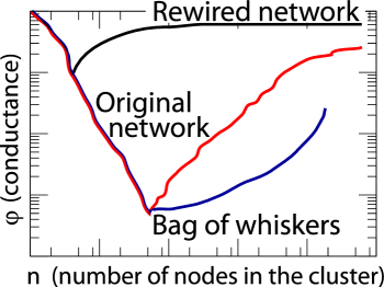
(a) Typical NCP plot

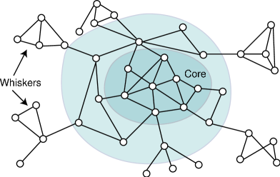
(b) Caricature of network structure

Figure 2: (a) Typical network community profile plot for a large social or information network: networks have better and better communities up to a size scale of $\approx 100$ nodes, and after that size scale communities “blend-in” with the rest of the network (red curve). However, real networks still have more structure than their randomized (conditioned on the same degree distribution) counterparts (black curve). Even more surprisingly, if one allows for disconnected communities (blue curve), the community quality scores often get even better (even though such communities have no intuitive meaning). (b) Network structure for a large social or information network, as suggested by our empirical evaluations. See the text for more information on the “core” and “whiskers,” and note that the core in our real-world networks is actually extremely sparse.

To understand the properties of generative models sufficient to reproduce the phenomena we have observed, we have examined in detail the structure of our social and information networks. Although nearly every network is an exception to any simple rule, we have observed that an “octopus” or “jellyfish” model [42, 152, 148] provides a rough first approximation to structure of many of the networks we have examined. That is, most networks may be viewed as having a “core,” with no obvious underlying geometry and which contains a constant fraction of the nodes, and then there is a periphery consisting of a large number of relatively small “whiskers” that are only tenuously connected to the core. Figure 2(b) presents a caricature of this network structure. Of course, our network datasets are far from random in numerous ways—e.g., they have higher edge density in the core; the small barely-connected whisker-like pieces are generally larger, denser, and more common than in corresponding random graphs; they have higher local clustering coefficients; and this local clustering information gets propagated globally into larger clusters or communities in a subtle and location-specific manner. More interestingly, as shown in Figure 13 in Section 4.4, the core itself consists of a nested core-periphery structure.

Main Modeling Results: The behavior that we observe is not reproduced, at even a qualitative level, by any of the commonly-used network generation models we have examined, including but not limited to preferential attachment models, copying models, small-world models, and hierarchical network models. Moreover, this behavior is qualitatively different than what is observed in networks with an underlying mesh-like or manifold-like geometry (which may not be surprising, but is significant insofar as these structures are often used as a scaffolding upon which to build other models), in networks that are good expanders (which may be surprising, since it is often observed that large social networks are expander-like), and in small social networks such as those used as testbeds for community detection algorithms (which may have implications for the applicability of these methods to detect large community-like structures in these networks). For the commonly-used network generation models, as well as for expander-like, low-dimensional, and small social networks, the network community profile plots are generally downward sloping or relatively flat.

Although it is well understood at a qualitative level that nodes that are “far apart” or “less alike” (in some sense) should be less likely to be connected in a generative model, understanding this point quantitatively so as to reproduce the empirically-observed relationship between small-scale and large-scale community structure turns out to be rather subtle. We can make the following observations:

• Very sparse random graph models with no underlying geometry have relatively deep cuts at small size scales, the best cuts at large size scales are very shallow, and there is a relatively abrupt transition in between. (This is shown pictorially in Figure 2(a) for a randomly rewired version of the original network.) This is a consequence of the extreme sparsity of the data: sufficiently dense random graphs do not have these small deep cuts; and the relatively deep cuts in sparse graphs are due to small tree-like pieces that are connected by a single edge to a core which is an extremely good expander.

• A Forest Fire generative model [112, 113], in which edges are added in a manner that imitates a fire-spreading process, reproduces not only the deep cuts at small size scales and the absence of deep cuts at large size scales but other properties as well: the small barely connected pieces are significantly larger and denser than random; and for appropriate parameter settings the network community profile plot increases relatively gradually as the size of the communities increases.

• The details of the “forest fire” burning mechanism are crucial for reproducing how local clustering information gets propagated to larger size scales in the network, and those details shed light on the failures of commonly-used network generation models. In the Forest Fire Model, a new node selects a “seed” node and links to it. Then with some probability it “burns” or adds an edge to the each of the seed’s neighbors, and so on, recursively. Although there is a “preferential attachment” and also a “copying” flavor to this mechanism, two factors are particularly important: first is the local (in a graph sense, as there is no underlying geometry in the model) manner in which the edges are added; and second is that the number of edges that a new node can add can vary widely, depending on the local structure around the seed node. Depending on the neighborhood structure around the seed, small fires will keep the community well-separated from the network, but occasional large fires will connect the community to the rest of the network and make it blend into the network core.

Thus, intuitively, the structure of the whiskers (components connected to the rest of the graph via a single edge) are responsible for the downward part of the network community profile plot, while the core of the network and the manner in which the whiskers root themselves to the core helps to determine the upward part of the network community profile plot. Due to local clustering effects, whiskers in real networks are larger and give deeper cuts than whiskers in corresponding randomized graphs, fluctuations in the core are larger and deeper than in corresponding randomized graphs, and thus the network community profile plot increases more gradually and levels off to a conductance value well below the value for a corresponding rewired network.

Main Methodological Contributions: To obtain these and other conclusions, we have employed approximation algorithms for graph partitioning to investigate structural properties of our network datasets. Briefly, we have done the following:

• We have used Metis+MQI, which consists of using the popular graph partitioning package Metis [95] followed by a flow-based MQI post-processing [106]. With this procedure, we obtain sets of nodes that have very good conductance scores. At very small size scales, these sets of nodes could plausibly be interpreted as good communities, but at larger size scales, we often obtain tenuously-connected (and in some cases unions of disconnected) pieces, which perhaps do not correspond to intuitive communities.

• Thus, we have also used the Local Spectral method of Anderson, Chung, and Lang [13] to obtain sets of nodes with good conductance value that that are “compact” or more “regularized” than those pieces returned by Metis+MQI. Since spectral methods confuse long paths with deep cuts [149, 84], empirically we obtain sets of nodes that have worse conductance scores than sets returned by Metis+MQI, but which are “tighter” and more “community-like.” For example, at small size scales the sets of nodes returned by the Local Spectral Algorithm agrees with the output of Metis+MQI, but at larger scales this algorithm returns sets of nodes with substantially smaller diameter and average diameter, which seem plausibly more community-like.

We have also used what we call the Bag-of-Whiskers Heuristic to identify small barely connected sets of nodes that exert a surprisingly large influence on the network community profile plot.

Both Metis+MQI and the Local Spectral Algorithm scale well and thus either may be used to obtain sets of nodes from very large graphs. For many of the small to medium-sized networks, we have checked our results by applying one or more other spectral, flow-based, or heuristic algorithms, although these do not scale as well to very large graphs. Finally, for some of our smaller network datasets, we have computed spectral-based and semidefinite-programming-based lower bounds, and the results are consistent with the conclusions we have drawn.

Broader implications: Our observation that, independently of the network size, compact communities exist only up to a size scale of around $100$ nodes agrees well with the “Dunbar number” [59], which predicts that roughly $150$ individuals is the upper limit on the size of a well-functioning human community. Moreover, we should emphasize that our results do not disagree with the literature at small sizes scales. One reason for the difference in our findings is that previous studies mainly focused on small networks, which are simply not large enough for the clusters to gradually blend into one another as one looks at larger size scales. In order to make our observations, one needs to look at large number (due to the complex noise properties of real graphs) of large networks. It is only when Dunbar’s limit is exceeded by several orders of magnitude that it is relatively easy to observe large communities blurring together and eventually vanishing. A second reason for the difference is that previous work did not measure and examine the network community profile of cluster size vs. cluster quality. Finally, we should note that our explanation also aligns well with the common bond vs. common identity theory of group attachment [141] from social psychology, where it has been noted that bond communities tend to be smaller and more cohesive [19], as they are based on interpersonal ties, while identity communities are focused around common theme or interest. We discuss these implications and connections further in Section 7.

1.3 Outline of the paper

The rest of the paper is organized as follows. In Section 2 we describe some useful background, including a brief description of the network datasets we have analyzed. Then, in Section 3 we present our main results on the properties of the network community profile plot for our network datasets. We place an emphasis on how the phenomena we observe in large social and information networks are qualitatively different than what one would expect based on intuition from and experience with expander-like graphs, low-dimensional networks, and commonly-studied small social networks. Then, in Sections 4 and 5, we summarize the results of additional empirical evaluations. In particular, in Section 4, we describe some of the observations we have made in an effort to understand what structural properties of these large networks are responsible for the phenomena we observe; and in Section 5, we describe some of the results of probing the networks with different approximation algorithms in an effort to be confident that the phenomena we observed really are properties of the networks we study, rather than artifactual properties of the algorithms we chose to use to study those networks. We follow this in Section 6 with a discussion of complex network generation models. We observe that the commonly-used network generation models fail to reproduce the counterintuitive phenomena we observe. We also notice that very sparse random networks reproduce certain aspects of the phenomena, and that a generative model based on an iterative “forest fire” burning mechanism reproduces very well the qualitative properties of the phenomena we observe. Finally, in Section 7 we provide a discussion of our results in a broader context, and in Section 8 we present a brief conclusion.

2 Background on communities and overview of our methods

In this section, we will provide background on our data and methods. We start in Section 2.1 with a description of the network datasets we will analyze. Then, in Section 2.2, we review related community detection and graph clustering ideas. Finally, in Section 2.3, we provide a brief description of approximation algorithms that we will use. There exist a large number of reviews on topics related to those discussed in this paper. For example, see the reviews on community identification [128, 53], data clustering [91], graph and spectral clustering [76, 154, 146], graph and heavy-tailed data analysis [129, 29, 50], surveys on various aspects of complex networks [10, 56, 127, 25, 52, 117, 23], the monographs on spectral graph theory and complex networks [34, 42], and the book on social network analysis [155]. See Section 7 for a more detailed discussion of the relationship of our work with some of this prior work.

2.1 Social and information network datasets we analyze

We have examined a large number of real-world complex networks. See Tables 1, 2, and 3 for a summary. For convenience, we have organized the networks into the following categories: Social networks; Information/citation networks; Collaboration networks; Web graphs; Internet networks; Bipartite affiliation networks; Biological networks; Low-dimensional networks; IMDB networks; and Amazon networks. We have also examined numerous small social networks that have been used as a testbed for community detection algorithms (e.g., Zachary’s karate club [160, 5], interactions between dolphins [119, 5], interactions between monks [145, 5], Newman’s network science network [130, 5], etc.), numerous simple network models in which by design there is an underlying geometry (e.g., power grid and road networks [156], simple meshes, low-dimensional manifolds including graphs corresponding to the well-studied “swiss roll” data set [153], a geometric preferential attachment model [71, 72], etc.), several networks that are very good expanders, and many simulated networks generated by commonly-used network generation models(e.g., preferential attachment models [127], copying models [102], hierarchical models [138], etc.).

Network	$N$	$E$	$N_{b}$	$E_{b}$	$\bar{d}$	$\tilde{d}$	$\bar{C}$	$D$	$\bar{D}$	Description
Social networks
Delicious	147,567	301,921	0.40	0.65	4.09	48.44	0.30	24	6.28	del.icio.us collaborative tagging social network
Epinions	75,877	405,739	0.48	0.90	10.69	183.88	0.26	15	4.27	Who-trusts-whom network from epinions.com [142]
Flickr	404,733	2,110,078	0.33	0.86	10.43	442.75	0.40	18	5.42	Flickr photo sharing social network [101]
LinkedIn	6,946,668	30,507,070	0.47	0.88	8.78	351.66	0.23	23	5.43	Social network of professional contacts
LiveJournal01	3,766,521	30,629,297	0.78	0.97	16.26	111.24	0.36	23	5.55	Friendship network of a blogging community [20]
LiveJournal11	4,145,160	34,469,135	0.77	0.97	16.63	122.44	0.36	23	5.61	Friendship network of a blogging community [20]
LiveJournal12	4,843,953	42,845,684	0.76	0.97	17.69	170.66	0.35	20	5.53	Friendship network of a blogging community [20]
Messenger	1,878,736	4,079,161	0.53	0.78	4.34	15.40	0.09	26	7.42	Instant messenger social network
Email-All	234,352	383,111	0.18	0.50	3.27	576.87	0.50	14	4.07	Research organization email network (all addresses) [113]
Email-InOut	37,803	114,199	0.47	0.82	6.04	165.73	0.58	8	3.74	(all addresses but email has to be sent both ways) [113]
Email-Inside	986	16,064	0.90	0.99	32.58	74.66	0.45	7	2.60	(only emails inside the research organization) [113]
Email-Enron	33,696	180,811	0.61	0.90	10.73	142.36	0.71	13	3.99	Enron email dataset [100]
Answers	488,484	1,240,189	0.45	0.78	5.08	251.78	0.11	22	5.72	Yahoo Answers social network
Answers-1	26,971	91,812	0.56	0.87	6.81	59.17	0.08	16	4.49	Cluster 1 from Yahoo Answers
Answers-2	25,431	65,551	0.48	0.80	5.16	56.57	0.10	15	4.76	Cluster 2 from Yahoo Answers
Answers-3	45,122	165,648	0.53	0.87	7.34	417.83	0.21	15	3.94	Cluster 3 from Yahoo Answers
Answers-4	93,971	266,199	0.49	0.82	5.67	94.48	0.08	16	4.91	Cluster 4 from Yahoo Answers
Answers-5	5,313	11,528	0.41	0.73	4.34	29.55	0.12	14	4.75	Cluster 5 from Yahoo Answers
Answers-6	290,351	613,237	0.40	0.71	4.22	57.16	0.09	22	5.92	Cluster 6 from Yahoo Answers
Information (citation) networks
Cit-Patents	3,764,105	16,511,682	0.82	0.96	8.77	21.34	0.09	26	8.15	Citation network of all US patents [112]
Cit-hep-ph	34,401	420,784	0.96	1.00	24.46	63.50	0.30	14	4.33	Citations between physics (arxiv hep-th) papers [78]
Cit-hep-th	27,400	352,021	0.94	0.99	25.69	106.40	0.33	15	4.20	Citations between physics (arxiv hep-ph) papers [78]
Blog-nat05-6m	29,150	182,212	0.74	0.96	12.50	342.51	0.24	10	3.40	Blog citation network (6 months of data) [116]
Blog-nat06all	32,384	315,713	0.87	0.99	19.50	153.08	0.20	18	3.94	Blog citation network (1 year of data) [116]
Post-nat05-6m	238,305	297,338	0.21	0.34	2.50	39.51	0.13	45	10.34	Blog post citation network (6 months) [116]
Post-nat06all	437,305	565,072	0.22	0.38	2.58	35.54	0.11	54	10.48	Blog post citation network (1 year) [116]
Collaboration networks
AtA-IMDB	883,963	27,473,042	0.87	0.99	62.16	517.40	0.79	15	3.48	IMDB actor collaboration network from Dec 2007
CA-astro-ph	17,903	196,972	0.89	0.98	22.00	65.70	0.67	14	4.21	Co-authorship in astro-ph of arxiv.org [112]
CA-cond-mat	21,363	91,286	0.81	0.93	8.55	22.47	0.70	15	5.36	Co-authorship in cond-mat category [112]
CA-gr-qc	4,158	13,422	0.64	0.78	6.46	17.98	0.66	17	6.10	Co-authorship in gr-qc category [112]
CA-hep-ph	11,204	117,619	0.81	0.97	21.00	130.88	0.69	13	4.71	Co-authorship in hep-ph category [112]
CA-hep-th	8,638	24,806	0.68	0.85	5.74	12.99	0.58	18	5.96	Co-authorship in hep-th category [112]
CA-DBLP	317,080	1,049,866	0.67	0.84	6.62	21.75	0.73	23	6.75	DBLP co-authorship network [20]

Table 1: Network datasets we analyzed. Statistics of networks we consider: number of nodes $N$; number of edges $E$; fraction nodes not in whiskers (size of largest biconnected component) $N_{b}/N$; fraction of edges in biconnected component $E_{b}/E$; average degree $\bar{d}=2E/N$; second order average degree $\tilde{d}$; average clustering coefficient $\bar{C}$; diameter $D$; and average path length $\bar{D}$.

Network	$N$	$E$	$N_{b}$	$E_{b}$	$\bar{d}$	$\tilde{d}$	$\bar{C}$	$D$	$\bar{D}$	Description
Web graphs
Web-BerkStan	319,717	1,542,940	0.57	0.88	9.65	1,067.55	0.32	35	5.66	Web graph of Stanford and UC Berkeley [98]
Web-Google	855,802	4,291,352	0.75	0.92	10.03	170.35	0.62	24	6.27	Web graph Google released in 2002 [3]
Web-Notredame	325,729	1,090,108	0.41	0.76	6.69	280.68	0.47	46	7.22	Web graph of University of Notre Dame [11]
Web-Trec	1,458,316	6,225,033	0.59	0.78	8.54	682.89	0.68	112	8.58	Web graph of TREC WT10G web corpus [2]
Internet networks
As-RouteViews	6,474	12,572	0.62	0.80	3.88	164.81	0.40	9	3.72	AS from Oregon Exchange BGP Route View [112]
As-Caida	26,389	52,861	0.61	0.81	4.01	281.93	0.33	17	3.86	CAIDA AS Relationships Dataset
As-Skitter	1,719,037	12,814,089	0.99	1.00	14.91	9,934.01	0.17	5	3.44	AS from traceroutes run daily in 2005 by Skitter
As-Newman	22,963	48,436	0.65	0.83	4.22	261.46	0.35	11	3.83	AS graph from Newman [5]
As-Oregon	13,579	37,448	0.72	0.90	5.52	235.97	0.46	9	3.58	Autonomous systems [1]
Gnutella-25	22,663	54,693	0.59	0.83	4.83	10.75	0.01	11	5.57	Gnutella network on March 25 2000 [143]
Gnutella-30	36,646	88,303	0.55	0.81	4.82	11.46	0.01	11	5.75	Gnutella P2P network on March 30 2000 [143]
Gnutella-31	62,561	147,878	0.54	0.81	4.73	11.60	0.01	11	5.94	Gnutella network on March 31 2000 [143]
eDonkey	5,792,297	147,829,887	0.93	1.00	51.04	6,139.99	0.08	5	3.66	P2P eDonkey graph for a period of 47 hours in 2004
Bi-partite networks
IpTraffic	2,250,498	21,643,497	1.00	1.00	19.23	94,889.05	0.00	5	2.53	IP traffic graph a single router for 24 hours
AtP-astro-ph	54,498	131,123	0.70	0.87	4.81	16.67	0.00	28	7.78	Authors-to-papers network of astro-ph [116]
AtP-cond-mat	57,552	104,179	0.65	0.79	3.62	10.54	0.00	31	9.96	Authors-to-papers network of cond-mat [116]
AtP-gr-qc	14,832	22,266	0.47	0.60	3.00	9.72	0.00	35	11.08	Authors-to-papers network of gr-qc [116]
AtP-hep-ph	47,832	86,434	0.60	0.76	3.61	16.80	0.00	27	8.55	Authors-to-papers network of hep-ph [116]
AtP-hep-th	39,986	64,154	0.53	0.68	3.21	13.07	0.00	36	10.74	Authors-to-papers network of hep-th [116]
AtP-DBLP	615,678	944,456	0.49	0.64	3.07	13.61	0.00	48	12.69	DBLP authors-to-papers bipartite network
Spending	1,831,540	2,918,920	0.34	0.58	3.19	1,536.35	0.00	26	5.62	Users-to-keywords they bid
Hw7	653,260	2,278,448	0.99	0.99	6.98	346.85	0.00	24	6.26	Downsampled advertiser-query bid graph
Netflix	497,959	100,480,507	1.00	1.00	403.57	28,432.89	0.00	5	2.31	Users-to-movies they rated. From Netflix prize [4]
QueryTerms	13,805,808	17,498,668	0.28	0.41	2.53	14.92	0.00	86	19.81	Users-to-queries they submit to a search engine
Clickstream	199,308	951,649	0.39	0.87	9.55	430.74	0.00	7	3.83	Users-to-URLs they visited [126]
Biological networks
Bio-Proteins	4,626	14,801	0.72	0.91	6.40	24.25	0.12	12	4.24	Yeast protein interaction network [51]
Bio-Yeast	1,458	1,948	0.37	0.51	2.67	7.13	0.14	19	6.89	Yeast protein interaction network data [92]
Bio-YeastP0.001	353	1,517	0.73	0.93	8.59	20.18	0.57	11	4.33	Yeast protein-protein interaction map [135]
Bio-YeastP0.01	1,266	8,511	0.79	0.97	13.45	47.73	0.44	12	3.87	Yeast protein-protein interaction map [135]

Table 2: Network datasets we analyzed. Statistics of networks we consider: number of nodes $N$; number of edges $E$; fraction nodes not in whiskers (size of largest biconnected component) $N_{b}/N$; fraction of edges in biconnected component $E_{b}/E$; average degree $\bar{d}=2E/N$; second order average degree $\tilde{d}$; average clustering coefficient $\bar{C}$; diameter $D$; and average path length $\bar{D}$.

Network	$N$	$E$	$N_{b}$	$E_{b}$	$\bar{d}$	$\tilde{d}$	$\bar{C}$	$D$	$\bar{D}$	Description
Nearly low-dimensional networks
Road-CA	1,957,027	2,760,388	0.80	0.85	2.82	3.17	0.06	865	310.97	California road network
Road-USA	126,146	161,950	0.97	0.98	2.57	2.81	0.03	617	218.55	USA road network (only main roads)
Road-PA	1,087,562	1,541,514	0.79	0.85	2.83	3.20	0.06	794	306.89	Pennsylvania road network
Road-TX	1,351,137	1,879,201	0.78	0.84	2.78	3.15	0.06	1,064	418.73	Texas road network
PowerGrid	4,941	6,594	0.62	0.69	2.67	3.87	0.11	46	19.07	Power grid of Western States Power Grid [156]
Mani-faces7k	696	6,979	0.98	0.99	20.05	37.99	0.56	16	5.52	Faces (64x64 grayscale images) (connect 7k closest pairs)
Mani-faces4k	663	3,465	0.90	0.97	10.45	20.20	0.56	29	8.96	Faces (connect 4k closest pairs)
Mani-faces2k	551	1,981	0.84	0.94	7.19	12.77	0.54	32	11.07	Faces (connect 2k closest pairs)
Mani-facesK10	698	6,935	1.00	1.00	19.87	25.32	0.51	6	3.25	Faces (connect every to 10 nearest neighbors)
Mani-facesK3	698	2,091	1.00	1.00	5.99	7.98	0.45	9	4.89	Faces (connect every to 5 nearest neighbors)
Mani-facesK5	698	3,480	1.00	1.00	9.97	12.91	0.48	7	4.03	Faces (connect every to 3 nearest neighbors)
Mani-swiss200k	20,000	200,000	1.00	1.00	20.00	21.08	0.59	103	37.21	Swiss-roll (connect 200k nearest pairs of nodes)
Mani-swiss100k	19,990	99,979	1.00	1.00	10.00	11.02	0.59	162	58.32	Swiss-roll (connect 100k nearest pairs of nodes)
Mani-swiss60k	19,042	57,747	0.93	0.96	6.07	7.03	0.59	243	89.15	Swiss-roll (connect 60k nearest pairs of nodes)
Mani-swissK10	20,000	199,955	1.00	1.00	20.00	25.38	0.56	10	5.47	Swiss-roll (every node connects to 10 nearest neighbors)
Mani-swissK5	20,000	99,990	1.00	1.00	10.00	12.89	0.54	13	8.34	Swiss-roll (every node connects to 5 nearest neighbors)
Mani-swissK3	20,000	59,997	1.00	1.00	6.00	7.88	0.50	17	6.89	Swiss-roll (every node connects to 3 nearest neighbors)
IMDB Actor-to-Movie graphs
AtM-IMDB	2,076,978	5,847,693	0.49	0.82	5.63	65.41	0.00	32	6.82	Actors-to-movies graph from IMDB (imdb.com)
Imdb-top30	198,430	566,756	0.99	1.00	5.71	18.19	0.00	26	8.32	Actors-to-movies graph heavily preprocessed
Imdb-raw07	601,481	1,320,616	0.54	0.79	4.39	20.94	0.00	32	8.55	Country clusters were extracted from this graph
Imdb-France	35,827	74,201	0.51	0.76	4.14	14.62	0.00	20	6.57	Cluster of French movies
Imdb-Germany	21,258	42,197	0.56	0.78	3.97	13.69	0.00	34	7.47	German movies (to actors that played in them)
Imdb-India	12,999	25,836	0.57	0.78	3.98	31.55	0.00	19	6.00	Indian movies
Imdb-Italy	19,189	37,534	0.55	0.77	3.91	11.66	0.00	30	6.91	Italian movies
Imdb-Japan	15,042	34,131	0.60	0.82	4.54	16.98	0.00	19	6.81	Japanese movies
Imdb-Mexico	13,783	36,986	0.64	0.86	5.37	24.15	0.00	19	5.43	Mexican movies
Imdb-Spain	15,494	31,313	0.51	0.76	4.04	14.22	0.00	28	6.44	Spanish movies
Imdb-UK	42,133	82,915	0.52	0.76	3.94	15.14	0.00	23	7.04	UK movies
Imdb-USA	241,360	530,494	0.51	0.78	4.40	25.25	0.00	30	7.63	USA movies
Imdb-WGermany	12,120	24,117	0.56	0.78	3.98	11.73	0.00	22	6.26	West German movies
Amazon product co-purchasing networks
Amazon0302	262,111	899,792	0.95	0.97	6.87	11.14	0.43	38	8.85	Amazon products from 2003 03 02 [49]
Amazon0312	400,727	2,349,869	0.94	0.99	11.73	30.33	0.42	20	6.46	Amazon products from 2003 03 12 [49]
Amazon0505	410,236	2,439,437	0.94	0.99	11.89	30.93	0.43	22	6.48	Amazon products from 2003 05 05 [49]
Amazon0601	403,364	2,443,311	0.96	0.99	12.11	30.55	0.43	25	6.42	Amazon products from 2003 06 01 [49]
AmazonAll	473,315	3,505,519	0.94	0.99	14.81	52.70	0.41	19	5.66	Amazon products (all 4 graphs merged) [49]
AmazonAllProd	524,371	1,491,793	0.80	0.91	5.69	11.75	0.35	42	11.18	Products (all products, source+target) [109]
AmazonSrcProd	334,863	925,872	0.84	0.91	5.53	11.53	0.43	47	12.11	Products (only source products) [109]

Table 3: Network datasets we analyzed. Statistics of networks we consider: number of nodes $N$; number of edges $E$; fraction nodes not in whiskers (size of largest biconnected component) $N_{b}/N$; fraction of edges in biconnected component $E_{b}/E$; average degree $\bar{d}=2E/N$; second order average degree $\tilde{d}$; average clustering coefficient $\bar{C}$; diameter $D$; and average path length $\bar{D}$.

Social networks: The class of social networks in Table 1 is particularly diverse and interesting. It includes several large on-line social networks: a network of professional contacts from LinkedIn (LinkedIn); a friendship network of a LiveJournal blogging community (LiveJournal01); and a who-trusts-whom network of Epinions (Epinions). It also includes an email network from Enron (Email-Enron) and from a large European research organization. For the latter we generated three networks: Email-Inside uses only the communication inside organization; Email-InOut also adds external email addresses where email has been sent both way; and Email-All adds all communication inside the organization and to the outside world. Also included in the class of social networks are networks that are not the central focus of the websites from which they come, but which instead serve as a tool for people to share information more easily. For example, we have: the networks of a social bookmarking site Delicious (Delicious); a Flickr photo sharing website (Flickr); and a network from Yahoo! Answers question answering website (Answers). In all these networks, a node refers to an individual and an edge is used to indicate that means that one person has some sort of interaction with another person, e.g., one person subscribes to their neighbor’s bookmarks or photos, or answers their questions.

Information and citation networks: The class of Information/citation networks contains several different citation networks. It contains two citation networks of physics papers on arxiv.org, (Cit-hep-th and Cit-hep-ph), and a network of citations of US patents (Cit-Patents). (These paper-to-paper citation networks are to be distinguished from scientific collaboration networks and author-to-paper bipartite networks, as described below.) It also contains two types of blog citation networks. In the so-called post networks, nodes are posts and edges represent hyperlinks between blog posts (Post-nat05-6m and Post-nat06all). On the other hand, the so-called blog network is the blog-level-aggregation of the same data, i.e., there is a link between two blogs if there is a post in first that links the post in a second blog (Blog-nat05-6m and Blog-nat06all).

Collaboration networks: The class of collaboration networks contain academic collaboration (i.e., co-authorship) networks between physicists from various categories in arxiv.org (CA-astro-ph, etc.) and between authors in computer science (CA-DBLP). It also contains a network of collaborations between pairs of actors in IMDB (AtA-IMDB), i.e., there is an edge connecting a pair of actors if they appeared in the same movie. (Again, this should be distinguished from actor-to-movie bipartite networks, as described below.)

Web graphs: The class of Web graph networks includes four different web-graphs in which nodes represent web-pages and edges represent hyperlinks between those pages. Networks were obtained from Google (Web-Google), the University of Notre Dame (Web-Notredame), TREC (Web-Trec), and Stanford University (Web-BerkStan). The class of Internet networks consists of various autonomous systems networks obtained at different sources, as well as a Gnutella and eDonkey peer-to-peer file sharing networks.

Bipartite networks: The class of Bipartite networks is particularly diverse and includes: authors-to-papers graphs from both computer science (AtP-DBLP) and physics (AtP-astro-ph, etc.); a network representing users and the URLs they visited (Clickstream); a network representing users and the movies they rated (Netflix); and a users-to-queries network representing query terms that users typed into a search engine (QueryTerms). (We also have analyzed several bipartite actors-to-movies networks extracted from the IMDB database, which we have listed separately below.)

Biological networks: The class of Biological networks include protein-protein interaction networks of yeast obtained from various sources.

Low dimensional grid-like networks: The class of Low-dimensional networks consists of graphs constructed from road (Road-CA, etc.) or power grid (PowerGrid) connections and as such might be expected to “live” on a two-dimensional surface in a way that all of the other networks do not. We also added a “swiss roll” network, a $2$-dimensional manifold embedded in $3$-dimensions, and a “Faces” dataset where each point is an $64$ by $64$ gray-scale image of a face (embedded in $4,096$ dimensional space) and where we connected the faces that were most similar (using the Euclidean distance).

IMDB, Yahoo! Answers and Amazon networks: Finally, we have networks from IMDB, Amazon, and Yahoo! Answers, and for each of these we have separately analyzed subnetworks. The IMDB networks consist of actor-to-movie links, and we include the full network as well as subnetworks associated with individual countries based on the country of production. For the Amazon networks, recall that Amazon sells a variety of products, and for each item $A$ one may compile the list the up to ten other items most frequently purchased by buyers of $A$. This information can be presented as a directed network in which vertices represent items and there is a edge from item $A$ to another item $B$ if $B$ was frequently purchased by buyers of $A$. We consider the network as undirected. We use five networks from a study of Clauset et al. [49], and two networks from the viral marketing study from Leskovec et al. [109]. Finally, for the Yahoo! Answers networks, we observe several deep cuts at large size scales, and so in addition the full network, we analyze the top six most well-connected subnetworks.

In addition to providing a brief description of the network, Tables 1, 2 and 3 show the number of nodes and edges in each network, as well as other statistics which will be described in Section 4.1. (In all cases, we consider the network as undirected, and we extract and analyze the largest connected component.) The sizes of these networks range from about $5,000$ nodes up to nearly $14$ million nodes, and from about $6,000$ edges up to more than $100$ million edges. All of the networks are quite sparse—their densities range from an average degree of about $2.5$ for the blog post network, up to an average degree of about $400$ in the network of movie ratings from Netflix, and most of the other networks, including the purely social networks, have average degree around $10$ (median average degree of $6$). In many cases, we examined several versions of a given network. For example, we considered the entire IMDB actor-to-movie network, as well as sub-pieces of it corresponding to different language and country groups. Detailed statistics for all these networks are presented in Tables 1, 2 and 3 and are described in Section 4. In total, we have examined over $100$ large real-world social and information networks, making this, to our knowledge, the largest and most comprehensive study of such networks.

2.2 Clusters and communities in networks

Hierarchical clustering is a common approach to community identification in the social sciences [155], but it has also found application more generally [80, 90]. In this procedure, one first defines a distance metric between pairs of nodes and then produces a tree (in either a bottom-up or a top-down manner) describing how nodes group into communities and how these group further into super-communities. A quite different approach that has received a great deal of attention (and that will be central to our analysis) is based on ideas from graph partitioning [146, 26]. In this case, the network is a modeled as simple undirected graph, where nodes and edges have no attributes, and a partition of the graph is determined by optimizing a merit function. The graph partitioning problem is find some number $k$ groups of nodes, generally with roughly equal size, such that the number of edges between the groups, perhaps normalized in some way, is minimized.

Let $G=(V,E)$ denote a graph, then the conductance $\phi$ of a set of nodes $S\subset V$, (where $S$ is assumed to contain no more than half of all the nodes), is defined as follows. Let $v$ be the sum of degrees of nodes in $S$, and let $s$ be the number of edges with one endpoint in $S$ and one endpoint in $\overline{S}$, where $\overline{S}$ denotes the complement of $S$. Then, the conductance of $S$ is $\phi=s/v$, or equivalently $\phi=s/(s+2e)$, where $e$ is the number of edges with both endpoints is $S$. More formally:

Definion 1

Given a graph $G$ with adjacency matrix $A$ the conductance of a set of nodes $S$ is defined as:

$$\phi(S)=\frac{\sum_{i\in S,j\notin S}A_{ij}}{\min\{A(S),A(\overline{S})\}},$$ (6)

where $A(S)=\sum_{i\in S}\sum_{j\in V}A_{ij}$, or equivalently $A(S)=\sum_{i\in S}d(i)$, where $d(i)$ is a degree of node $i$ in $G$. Moreover, in this case, the conductance of the graph $G$ is:

$$\phi_{G}=\min_{S\subset V}\phi(S).$$ (7)

Thus, the conductance of a set provides a measure for the quality of the cut $(S,\overline{S})$, or relatedly the goodness of a community $S$.

Indeed, it is often noted that communities should be thought of as sets of nodes with more and/or better intra-connections than inter-connections; see Figure 3 for an illustration. When interested in detecting communities and evaluating their quality, we prefer sets with small conductances, i.e., sets that are densely linked inside and sparsely linked to the outside. Although numerous measures have been proposed for how community-like is a set of nodes, it is commonly noted—e.g., see Shi and Malik [147] and Kannan, Vempala, and Vetta [93]—that conductance captures the “gestalt” notion of clustering [161], and as such it has been widely-used for graph clustering and community detection [76, 154, 146].

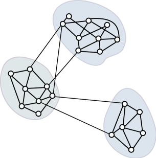
(a) Three communities

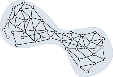
(b) Conductance bottleneck

Figure 3: (a) Caricature of the traditional view of communities as being sets of nodes with more and/or better intra-connections than inter-connections. (b) A graph with its minimum conductance bottleneck illustrated.

There are many other density-based measures that have been used to partition a graph into a set of communities [76, 154, 146]. One that deserves particular mention is modularity [132, 131]. For a given partition of a network into a set of communities, modularity measures the number of within-community edges, relative to a null model that is usually taken to be a random graph with the same degree distribution. Thus, modularity was originally introduced and it typically used to measure the strength or quality of a particular partition of a network. We, however, are interested in a quite different question than those that motivated the introduction of modularity. Rather than seeking to partition a graph into the “best” possible partition of communities, we would like to know how good is a particular element of that partition, i.e., how community-like are the best possible communities that modularity or any other merit function can hope to find, in particular as a function of the size of that partition.

2.3 Approximation algorithms for finding low-conductance cuts

In addition to capturing very well our intuitive notion of what it means for a set of nodes to be a good community, the use of conductance as an objective function has an added benefit: there exists an extensive theoretical and practical literature on methods for approximately optimizing it. (Finding cuts with exactly minimal conductance is NP-hard.) In particular, the theory literature contains several algorithms with provable approximation performance guarantees.

First, there is the spectral method, which uses an eigenvector of the graph’s Laplacian matrix to find a cut whose conductance is no bigger than $\phi$ if the graph actually contains a cut with conductance $O(\phi^{2})$ [32, 55, 66, 123, 34]. The spectral method also produces lower bounds which can show that the solution for a given graph is closer to optimal than promised by the worst-case guarantee. Second, there is an algorithm that uses multi-commodity flow to find a cut whose conductance is within an $O(\log n)$ factor of optimal [107, 108]. Spectral and multi-commodity flow based methods are complementary in that the worst-case $O(\log n)$ approximation factor is obtained for flow-based methods on expander graphs [107, 108], a class of graphs which does not cause problems for spectral methods, whereas spectral methods can confuse long path with deep cuts [84, 149], a difference that does not cause problems for flow-based methods. Third, and very recently, there exists an algorithm that uses semidefinite programming to find a solution that is within $O(\sqrt{\log n})$ of optimal [17]. This paper sparked a flurry of theoretical research on a family of closely related algorithms including [15, 99, 16], all of which can be informally described as combinations of spectral and flow-based techniques which exploit their complementary strengths. However, none of those algorithms are currently practical enough to use in our study.

Of the above three theoretical algorithms, the spectral method is by far the most practical. Also very common are recursive bisection heuristics: recursively divide the graph into two groups, and then further subdivide the new groups until the desired number of clusters groups is achieved. This may be combined with local improvement methods like the Kernighan-Lin and Fiduccia-Mattheyses procedures [97, 65], which are fast and can climb out of some local minima. The latter was combined with a multi-resolution framework to create Metis [95, 96], a very fast program intended to split mesh-like graphs into equal sized pieces. The authors of Metis later created Cluto [162], which is better tuned for clustering-type tasks. Finally we mention Graclus [54], which uses multi-resolution techniques and kernel $k$-means to optimize a metric that is closely related to conductance.

While the preceding were all approximate algorithms for finding the lowest conductance cut in a whole graph, we now mention MQI [77, 106], an exact algorithm for the slightly different problem of finding the lowest conductance cut in half of a graph. This algorithm can be combined with a good method for initially splitting the graph into two pieces (such as Metis or the Spectral method) to obtain a surprisingly strong heuristic method for finding low conductance cuts in the whole graph [106]. The exactness of the second optimization step frequently results in cuts with extremely low conductance scores, as will be visible in many of our plots. MQI can be implemented by solving single parametric max flow problems, or sequences of ordinary max flow problems. Parametric max flow (with MQI described as one of the applications) was introduced by [77], and recent empirical work is described in [18], but currently there is no publicly available code that scales to the sizes we need. Ordinary max flow is a very thoroughly studied problem. Currently, the best theoretical time bounds are [82], the most practical algorithm is [83], while the best implementation is hi_pr by [33]. Since Metis+MQI using the hi_pr code is very fast and scalable, while the method empirically seems to usually find the lowest or nearly lowest conductance cuts in a wide variety of graphs, we have used it extensively in this study.

We will also extensively use Local Spectral Algorithm of Andersen, Chung, and Lang [13] to find node sets of low conductance, i.e., good communities, around a seed node. This algorithm is also very fast, and it can be successfully applied to very large graphs to obtain more “well-rounded”, “compact,” or “evenly-connected” communities than those returned by Meits+MQI. The latter observation (described in more detail in Section 5) is since local spectral methods also confuse long paths (which tend to occur in our very sparse network datasets) with deep cuts. This algorithm takes as input two parameters—the seed node and a parameter $\epsilon$ that intuitively controls the locality of the computation—and it outputs a set of nodes. Local spectral methods were introduced by Spielman and Teng [150, 13], and they have roughly the same kind of quadratic approximation guarantees as the global spectral method, but they have computational cost is proportional to the size of the obtained piece [35, 37, 36].

3 The Network Community Profile Plot (NCP plot)

In this section, we discuss the network community profile plot (NCP plot), which measures the quality of network communities at different size scales. We start in Section 3.1 by introducing it. Then, in Section 3.2, we present the NCP plot for several examples of networks which inform peoples’ intuition and for which the NCP plot behaves in a characteristic manner. Then, in Sections 3.3 and 3.4 we present the NCP plot for a wide range of large real world social and information networks. We will see that in such networks the NCP plot behaves in a qualitatively different manner.

3.1 Definitions for the network community profile plot

In order to more finely resolve community structure in large networks, we introduce the network community profile plot (NCP plot). Intuitively, the NCP plot measures the quality of the best possible community in a large network, as a function of the community size. Formally, we may define it as the conductance value of the best conductance set of cardinality $k$ in the entire network, as a function of $k$.

Definion 2

Given a graph $G$ with adjacency matrix $A$, the network community profile plot (NCP plot) plots $\Phi(k)$ as a function of $k$, where

$$\Phi(k)=\min_{S\subset V,|S|=k}\phi(S),$$ (8)

where $|S|$ denotes the cardinality of the set $S$, and where the conductance $\phi(S)$ of $S$ is given by equation (6).

Since this quantity is intractable to compute, we will employ well-studied approximation algorithms for the Minimum Conductance Cut Problem to approximate it. In particular, operationally we will use several natural heuristics based on approximation algorithms to do graph partitioning in order to compute different approximations to the NCP plot. Although other procedures will be described in Section 5, we will primarily employ two procedures. First, Metis+MQI, i.e., the graph partitioning package Metis [95] followed by the flow-based post-processing procedure MQI [106]; this procedure returns sets that have very good conductance values. Second, the Local Spectral Algorithm of Andersen, Chung, and Lang [13]; this procedure returns sets that are somewhat more “compact” or “smoothed” or “regularized,” but that often have somewhat worse conductance values.

Just as the conductance of a set of nodes provides a quality measure of that set as a community, the shape of the NCP plot provides insight into the community structure of a graph as a whole. For example, the magnitude of the conductance tells us how well clusters of different sizes are separated from the rest of the network. One might hope to obtain some sort of “smoothed” measure of the notion of the best community of size $k$ (e.g., by considering an average of the conductance value over all sets of a given size or by considering a smoothed extremal statistic such as a $95$-th percentile) rather than conductance of the best set of that size. We have not defined such a measure since there is no obvious way to average over all subsets of size $k$ and obtain a meaningful approximation to the minimum. On the other hand, our approximation algorithm methodology implicitly incorporates such an effect. Although Metis+MQI finds sets of nodes with extremely good conductance value, empirically we observe that they often have little or no internal structure—they can even be disconnected. On the other hand, since spectral methods in general tend to confuse long paths with deep cuts [149, 84], the Local Spectral Algorithm finds sets that are “tighter” and more “well-rounded” and thus in many ways more community-like. (See Sections 2.3 and 5 for details on these algorithmic issues and interpretations.)

3.2 Community profile plots for expander, low-dimensional, and small social networks

The NCP plot behaves in a characteristic manner for graphs that are “well-embeddable” into an underlying low-dimensional geometric structure. To illustrate this, consider Figure 4. In Figure 4(a), we show the results for a $1$-dimensional chain, a $2$-dimensional grid, and a $3$-dimensional cube. In each case, the NCP plot is steadily downward sloping as a function of the number of nodes in the smaller cluster. Moreover, the curves are straight lines with a slope equal to $-1/d$, where $d$ is the dimensionality of the underlying grids. In particular, as the underlying dimension increases then the slope of the NCP plot gets less steep. Thus, we observe:

Observation 1

If the network under consideration corresponds to a $d$-dimensional grid, then the NCP plot shows that

$$-\frac{1}{d}=\frac{\log(\phi(k))}{\log(k)}.$$ (9)

This is simply a manifestation of the isoperimetric (i.e., surface area to volume) phenomenon: for a grid, the “best” cut is obtained by cutting out a set of adjacent nodes, in which case the surface area (number of edges cut) increases as $O(m^{d-1}$), while the volume (number of vertices/edges inside the cluster) increases as $O(m^{d})$.

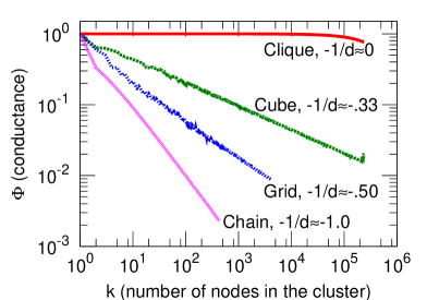
(a) Several low-dimensional meshes.

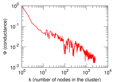
(b) PowerGrid

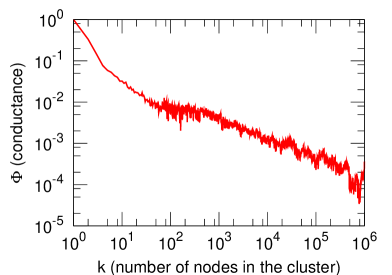
(c) Road-CA

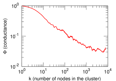
(d) Manifold

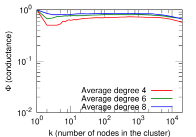
(e) Expander: dense $G_{nm}$ graph

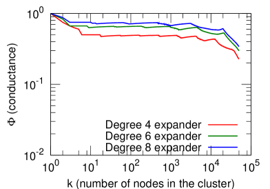
(f) Expander: union of matchings

Figure 4: Network community profile plots for expander-like graphs and several networks that “live” in low-dimensional spaces. (4(a)) A large clique graph, a cube (3d mesh), a grid (2d mesh) and a chain (line). Note that the slope of community profile plot directly corresponds to dimensionality of the graph. (4(b)) and (4(c)) Two networks on the Earth’s surface and thus that are reasonably well-embeddable in two dimensions. (4(d)) A 2d “swiss roll” manifold embedded in $3$ dimensions, where every we connected every point to $10$ nearest neighbors. (4(e)) and (4(f)) Two networks that are very good expanders.

This qualitative phenomenon of a steadily downward sloping NCP plot is quite robust for networks that “live” in a low-dimensional structure, e.g., on a manifold or the surface of the earth. For example, Figure 4(b) shows the NCP plot for a power grid network of Western States Power Grid [156], and Figure 4(c) shows the NCP plot for a road network of California. These two networks have very different sizes—the power grid network has $4,941$ nodes and $6,594$ edges, and the road network has $1,957,027$ nodes and $2,760,388$ edges—and they arise in very different application domains. In both cases, however, we see predominantly downward sloping NCP plot, very much similar to the profile of a simple $2$-dimensional grid. Indeed, the “best-fit” line for power grid gives the slope of $\approx-0.45$, which by (9) suggests that $d\approx 2.2$, which is not far from the “true” dimensionality of $2$. Moreover, empirically we observe that minima in the NCP plot correspond to community-like sets, which are occasionally nested. This corresponds to hierarchical community organization. For example, the nodes giving the dip at $k=19$ are included in the nodes giving the dip at $k=883$, while dips at $k=94$ and $k=105$ are both included in the dip at $k=262$.

In a similar manner, Figure 4(d) shows the profile plot for a graph generated from a “swiss roll” dataset which is commonly examined in the manifold and machine learning literature [153]. In this case, we still observe a downward sloping NCP plot that corresponds to internal dimensionally of the manifold (2 in this case). Finally, Figures 4(e) and 4(f) show NCP plots for two graphs that are very good expanders. The first is a $G_{nm}$ graph with $100,000$ nodes and a number of edges such that the average degree is $4$, $6$, and $8$. The second is a constant degree expander: to make one with degree $d$, we take the union of $d$ disjoint but otherwise random complete matchings, and we have plotted the results for $d=4,6,8$. In both of these cases, the NCP plot is roughly flat, which we also observed in Figure 4(a) for a clique, which is to be expected since the minimum conductance cut in the entire graph cannot be too small for a good expander [88].

Somewhat surprisingly (especially when compared with large networks in Section 3.3), a steadily decreasing downward NCP plot is seen for small social networks that have been extensively studied in validating community detection algorithms. Several examples are shown in Figures 5. For these networks, the interpretation is similar to that for the low-dimensional networks: the downward slope indicates that as potential communities get larger and larger, there are relatively more intra-edges than inter-edges; and empirically we observe that local minima in the NCP plot correspond to sets of nodes that are plausible communities. Consider, e.g., Zachary’s karate club [160] network (ZacharyKarate), an extensively-analyzed social network [128, 131, 94]. The network has $34$ nodes, each of which represents a member of a karate club, and $78$ edges, each of which represent a friendship tie between two members. Figure 5(a) depicts the karate club network, and Figure 5(b) shows its NCP plot. There are two local minima in the plot: the first dip at $k=5$ corresponds to the Cut $A$, and the second dip at $k=17$ corresponds to Cut $B$. Note that Cut $B$, which separates the graph roughly in half, has better conductance value than Cut $A$. This corresponds with the intuition about the NCP plot derived from studying low-dimensional graphs. Note also that the karate network corresponds well with the intuitive notion of a community, where nodes of the community are densely linked among themselves and there are few edges between nodes of different communities.

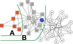
(a) Zachary’s karate club network …

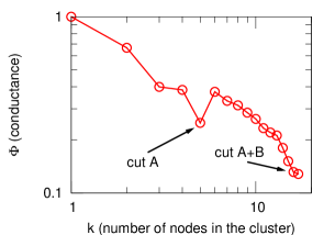
(b) …and it’s community profile plot

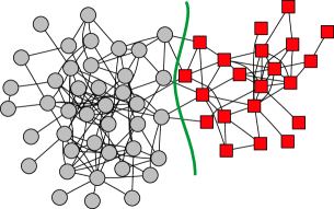
(c) Dolphins social network …

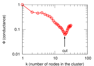
(d) …and it’s community profile plot

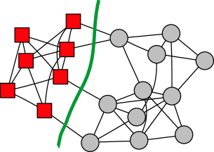
(e) Monks social network …

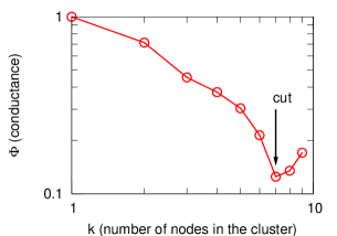
(f) …and it’s community profile plot

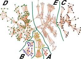
(g) Network science network …

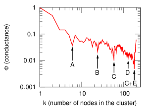
(h) …and it’s community profile plot

Figure 5: Depiction of several small social networks that are common test sets for community detection algorithms and their network community profile plots. (5(a)–5(b)) Zachary’s karate club network. (5(c)–5(d)) A network of dolphins. (5(e)–5(f)) A network of monks. (5(g)–5(h)) A network of researchers researching networks.

In a similar manner: Figure 5(c) shows a social network (with $62$ nodes and $159$ edges) of interactions within a group of dolphins [119]; Figure 5(e) shows a social network of monks (with $18$ nodes representing individual monks and $41$ edges representing social ties between pairs of monks) in a cloister [145]; and Figure 5(g) depicts Newman’s network (with $914$ collaborations between $379$ researchers) of scientists who conduct research on networks [132]. For each network, the NCP plot exhibits a downward trend, and it has local minima at cluster sizes that correspond to good communities: the minimum for the dolphins network (Figure 5(d)) corresponds to the separation of the network into two communities denoted with different shape and color of the nodes (gray circles versus red squares); the minima of the monk network (Figure 5(f)) corresponds to the split of $7$ Turks (red squares) and the so-called loyal opposition (gray circles) [145]; and empirically both local minima and the global minimum in the network science network (Figure 5(h)) correspond to plausible communities. Note that in the last case, the figure also displays hierarchical structure in which case the community defined by Cut $C$ is included in a larger community that has better conductance value.

At this point, we can observe that the following two general observations hold for networks that are well-embeddable in a low-dimensional space and also for small social networks that have been extensively studied and used to validate community detection algorithms. First, minima in the NCP plots, i.e., the best low-conductance cuts of a given size, correspond to communities-like sets of nodes. Second, the NCP plots are generally relatively gradually sloping downwards, meaning that smaller communities can be combined into larger sets of nodes that can also be meaningfully interpreted as communities.

3.3 Community profile plots for large social and information networks

We have examined NCP plots for each of the networks listed in Tables 1, 2 and 3. In Figure 6, we present NCP plots for six of these networks. (These particular networks were chosen to be representative of the wide range of networks we have examined, and for ease of comparison we will compute other properties for them in future sections. See Figures 7, 8, and 9 in Section 3.4 for the NCP plots of other networks listed in Tables 1, 2 and 3, and for a discussion of them.) The most striking feature of these plots is that the NCP plot is steadily increasing for nearly its entire range.

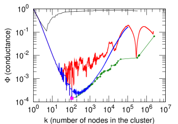
(a) LiveJournal01

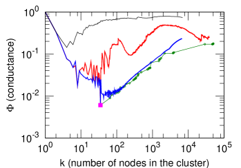
(b) Epinions

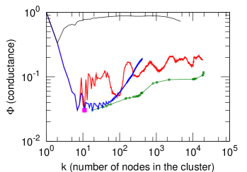
(c) Cit-hep-th

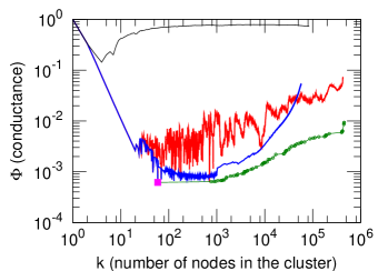
(d) Web-Google

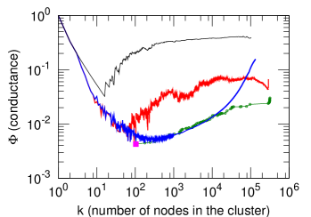
(e) Atp-DBLP

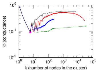
(f) Gnutella-31

Figure 6: [Best viewed in color.] Network community profile plots for a representative sample of large networks listed in Tables 1, 2 and 3. The red curves plot the results of the Local Spectral Algorithm on the specified network; green curves plot the results of Metis+MQI; blue curves plot the results of the Bag-of-Whiskers Heuristic; and black curves plot the results of the Local Spectral Algorithm applied to a randomly rewired version of the same network. Notice that in all cases the “best” communities are quite small (typically between $10$ and $100$ nodes) and that the network community profile plot steadily increases for nearly its entire range. See Figures 7, 8, and 9 for the NCP plots of other networks.

Consider, first, the NCP plot for the LiveJournal01 social network, as shown in Figure 6(a), and focus first on the red curve, which presents the results of applying the Local Spectral Algorithm. We make the following observations:

• Up to a size scale, which empirically is roughly $100$ nodes, the slope of the NCP plot is generally sloping downward.

• At that size scale, we observe the global minimum of the NCP plot. This set of nodes as well as others achieving local minima of the NCP plot in the same size range are the “best” communities, according to the conductance measure, in the entire graph.

• These best communities (the best denoted by a square) are barely connected to the rest of the graph, e.g., they are typically connected to the rest of the nodes by a single edge.

• Above the size scale of roughly $100$ nodes, the NCP plot gradually increases over several orders of magnitude. The “best” communities in the entire graph are quite good (in that they have size roughly $10^{2}$ nodes and conductance scores less than $10^{-3}$) whereas the “best” communities of size $10^{5}$ or $10^{6}$ have conductance scores of about $10^{-1}$. In between these two size extremes, the conductance scores get gradually worse, although there are numerous local dips and even one relatively large dip between $10^{5}$ and $10^{6}$ nodes.

Note that both axes in Figure 6 are logarithmic, and thus the upward trend of the NCP plot is over a wide range of size scales. Note also that the green curve plots the results of Metis+MQI (that returns disconnected clusters), and the blue curve plots the results of applying the Bag-of-Whiskers Heuristic, as described in Section 4.3. These procedures will be discussed in detail in Sections 4 and 5.

The black curve in Figure 6(a) plots the results of the Local Spectral Algorithm applied to a rewired version of the LiveJournal01 network, i.e., to a random graph conditioned on the same degree distribution as the original network. (We obtain such random graph by starting with the original network and then randomly selecting pairs of edges and rewiring the endpoints. By doing the rewiring long enough, we obtain a random graph that has the same degree sequence as the original network [122].)

Interestingly, the NCP of a rewired network first slightly decreases but then increases and flattens out. Several things should be noted:

• The original LiveJournal01 network has considerably more structure, i.e., deeper/better cuts, than its rewired version, even up to the largest size scales. That is, we observe significantly more structure than would be seen, for example, in an random graph on the same degree sequence.

• Relative to the original network, the “best” community in the rewired graph, i.e., the global minimum of the conductance curve, shifts upward and towards the left. This means that in rewired networks the best conductance clusters get smaller and have worse conductance scores.

• Sets at and near the minimum are small trees that are connected to the core of the random graph by a single edge.

• After the small dip at a very small size scale ($\approx 10$ nodes), the NCP plot increases to a high level rather quickly. This is due to the absence of structure in the core.

Finally, also note that the variance in the rewired version of the NCP plot (data not shown) is not much larger than the width of the curve in the figure.

We have observed qualitatively similar results in nearly every large social and information network we have examined. For example, several additional examples are presented in Figure 6: another network from the class of social networks (Epinions, in Figure 6(b)); an information/citation network (Cit-hep-th, in Figure 6(c)); a Web graph (Web-Google, in Figure 6(d)); a Bipartite affiliation network (AtP-DBLP, in Figure 6(e)); and an Internet network (Gnutella-31, in Figure 6(f)).

Qualitative observations are consistent across the range of network sizes, densities, and different domains from which the networks are drawn. Of course, these six networks are very different than each other—some of these differences are hidden due to the definition of the NCP plot, whereas others are evident. Perhaps the most obvious example of the latter is that even the best cuts in Gnutella-31 are not significantly smaller or deeper than in the corresponding rewired network, whereas for Web-Google we observe cuts that are orders of magnitude deeper.

Intuitively, the upward trend in the NCP plot means that separating large clusters from the rest of the network is especially expensive. It suggests that larger and larger clusters are “blended in” more and more with the rest of the network. The interpretation we draw, based on these data and data presented in subsequent sections is that, if a density-based concept such as conductance captures our intuitive notion of community goodness and if we model large networks with interaction graphs, then the best possible communities get less and less community-like as they grow in size.

3.4 More community profile plots for large social and information networks

Figures 7, 8, and 9 show additional examples of NCP plots for networks from Tables 1, 2 and 3. In the first two rows of Figure 7, we have several examples of purely Social networks and two email networks, in the third row we have patent and blog Information/citation networks, and in the final row we have three examples of actor and author Collaboration networks. In Figure 8, we see three examples each of Web graphs, Internet networks, Bipartite affiliation networks, and Biological networks. Finally, in the first row of Figure 9, we see Low-dimensional networks, including two road and a manifold network; in the second row, we have an IMDB Actor-to-Movie graphs and two subgraphs induced by restricting to individual countries; in the third row, we see three Amazon product co-purchasing networks; and in the final row we see a Yahoo! Answers networks and two subgraphs that are large good conductance cuts from the full network.

Social networks
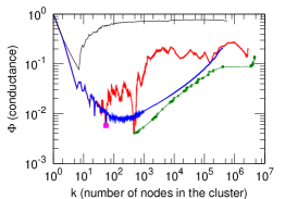
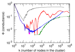
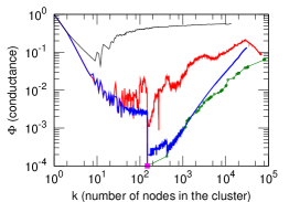
LinkedIn	Messenger	Delicious
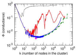
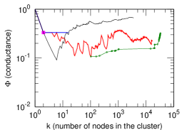
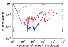
Flickr	Email-InOut	Email-enron
Information networks (citation and blog networks)
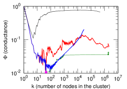
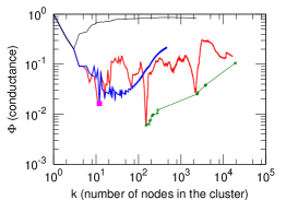
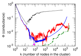
Patents	Blog-nat06all	Post-nat06all
Collaboration networks
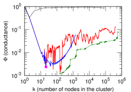
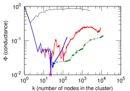
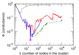
AtA-IMDB	CA-astro-ph	CA-hep-ph

Figure 7: [Best viewed in color.] Community profile plots of networks from Table 1.

Web graphs
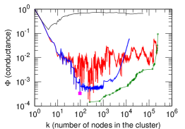
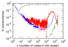
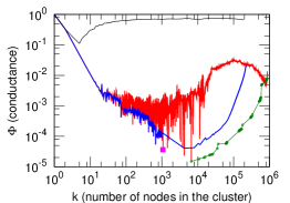
Web-BerkStan	Web-Notredame	Web-Trec
Internet networks
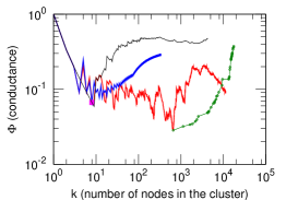
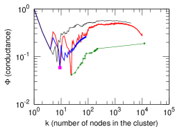
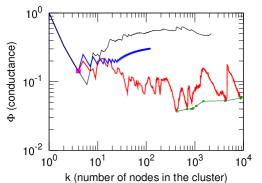
As-Newman	Gnutella-25	As-Oregon
Bipartite affiliation networks
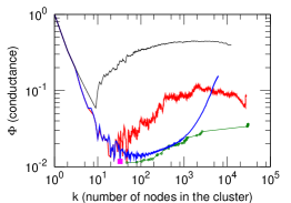
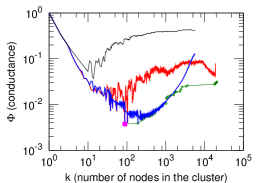
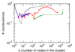
AtP-cond-mat	AtP-hep-th	Clickstream
Biological networks
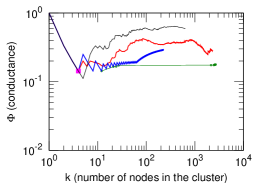
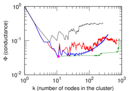
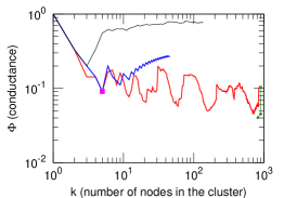
Bio-Proteins	Bio-Yeast	Bio-YeastP0.01

Figure 8: [Best viewed in color.] Community profile plots of networks from Table 2.

Low-dimensional networks
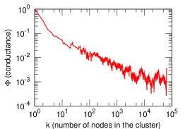
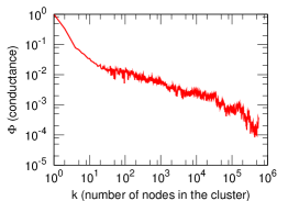
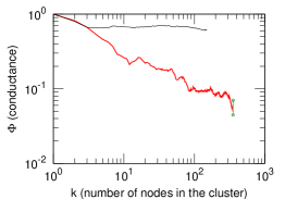
Road-USA	Road-PA	Mani-facesK5
IMDB Actor-to-Movie graphs
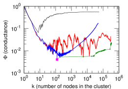
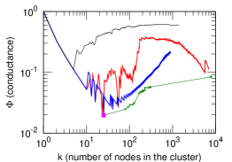
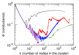
Imdb-raw07	Imdb-Mexico	Imdb-WGermany
Amazon product co-purchasing networks
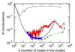
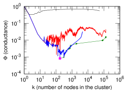
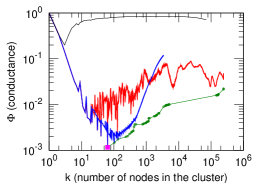
AmazonAllProd	Amazon0302	AmazonAll
Yahoo Answers networks
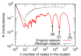
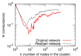
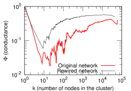
Answers	Answers-5	Answers-6

Figure 9: [Best viewed in color.] Community profile plots of networks from Table 3, as well as Answers and two sub-pieces of Answers.

For most of these networks, the same four versions of the NCP plot are plotted that were presented in Figure 6. Note that, as before, the scale of the vertical axis in these graphs is not all the same; the minima range from $10^{-2}$ to $10^{-5}$. These network datasets are drawn from a wide range of areas, and these graphs contain a wealth of information, a full analysis of which is well beyond the scope of the paper. Note, however, that the general trends we discussed in Section 3.3 still manifest themselves in nearly every network.

The Imdb-raw07 network is interesting in that its NCP plot does not increase much (at least not the version computed by the Local Spectral Algorithm) and we clearly observe large sets with good conductance values. Upon examination, many of the large good conductance cuts seem to be associated with different language groups. Two things should be noted. First, and not surprisingly, in this network and others, we have observed that there is some sensitivity to how the data are prepared. For example, we obtain somewhat stronger communities if ambiguous nodes (and there are a lot of ambiguous nodes in network datasets with millions of nodes) are removed than if, e.g., they are assigned to a country based on a voting mechanism of some other heuristic. A full analysis of these data preparation issues is beyond the scope of this paper, but our overall conclusions seem to hold independent of the preparation details. Second, if we examine individual countries—two representative examples are shown—then we see substantially less structure at large size scales.

The Yahoo! Answers social network (see Answers) also has several large cuts with good conductance value—actually, the best cut in the network has more $10^{5}$ nodes. (It is likely that exogenous factors are responsible for these large deep cuts.) Using standard graph partitioning procedures, we obtained four large disjoint clusters consisting of ca. $5,300$, $25,400$, $27,000$, and $290,000$ nodes, respectively, corresponding to the four dips (two of which visually overlap) in the NCP plot. We then examined the community profile plots for each of these pieces. The two representative examples of which we show clearly indicate a NCP plot that is much more like other network datasets we have examined.

4 More structural observations of our network datasets

We have examined in greater detail our network datasets in order to understand which structural properties are responsible for the observed properties of the NCP plot. We first present statistics for our network datasets in Section 4.1. Then, in Section 4.2 we describe a heuristic to identify small sets of nodes that have strong connections amongst themselves but that are connected to the remainder of the network by only a single edge. In Section 4.3, we show that these “whiskers” (or disjoint unions of them) are often the “best” conductance communities in the network. Last, in Section 4.4 we examine NCP plots for networks in which these whiskers have been removed.

4.1 General statistics on our network datasets

In Tables 1, 2, and 3, we also present the following statistics for our network datasets: the number of nodes $N$; the number of edges $E$; the fraction of nodes in the largest biconnected component $N_{b}/N$; the fraction of edges in the largest biconnected component $E_{b}/E$; the average degree $\bar{d}=2E/N$; the empirical second-order average degree [42] $\tilde{d}$; average clustering coefficient [156] $\bar{C}$; the estimated diameter $D$; and the estimated average path length $\bar{D}$. (The diameter was estimated using the following algorithm: pick a random node, find the farthest node $X$ (via shortest path); move to $X$ and find the farthest node from $X$; iterate this procedure until the distance to the farthest node does not increase anymore. The average path length was estimated based on $10,000$ randomly sampled nodes.)

In nearly every network we have examined, there is a substantial fraction of nodes that are barely connected to the main part of the network, i.e., that are part of a small cluster of ca. $10$ to $100$ nodes that are attached to the remainder of the network via one or a small number of edges. In particular, a large fraction of the network is made out of nodes that are not in the biconnected core.

For example, the Epinions network has $75,877$ nodes and $405,739$ edges, and the core of the network has only $36,111$ ($47\%$) nodes and $365,253$ ($90\%$) edges. For Delicious, the core is even smaller: it contains only $40\%$ of the nodes, and $65\%$ of the edges. Averaging over our network datasets, we see that the largest biconnected component contains around only $60\%$ of the nodes and $80\%$ of the edges of the original network. This is somewhat akin to the so-called “Jellyfish” model [152, 148] (which was proposed as a model for the graph of internet topology) and also to the “Octopus” model (for random power law graphs [42], which is described in more detail in Section 6.2). Moreover, the global minimum of the NCP plot is nearly always one of these pieces that is connected by only a single edge. Since these small barely-connected pieces seem to have a disproportionately large influence on the community structure of our network datasets, we examine them in greater detail in the next section.

4.2 Network “whiskers” and the “core”

We define whiskers, or more precisely $1$-whiskers, to be maximal subgraphs that can be detached from the rest of the network by removing a single edge. (Occasionally, we use the term whiskers informally to refer to barely connected sets of nodes more generally.) To find $1$-whiskers, we employ the following algorithm. Using a depth-first search algorithm, we find the largest biconnected component $B$ of the graph $G$. (A graph is biconnected if the removal of any single edge does not disconnect the graph.) We then delete all the edges in $G$ that have one of their end points in $B$. We call the connected components of this new graph $G^{\prime}$ $1$-whiskers, since they correspond to largest subgraphs that can be disconnected from $G$ by removing just a single edge. Recall that Figure 2(b) contains a schematic picture a network, including several of its whiskers.

Not surprisingly, there is a wide range of whisker sizes and shapes. Figure 10 shows the distribution of $1$-whisker sizes for a representative selection of our network datasets. Empirically, $1$-whisker size distribution is heavy-tailed, with the largest whisker size ranging from around less than $10$ to well above $100$. The largest whiskers in co-authorship and citation networks have around $10$ nodes, whiskers in bipartite graphs also tend to be small, and very large whiskers are found in a web graph. Figure 10 also compares the size of the whiskers with the sizes of whiskers in a rewired version of the same network. (The first thing to note is that due to the sparsity of the networks, the rewired versions all have whiskers.) In rewired networks the whiskers tend to be much smaller than in the original network. A particularly noteworthy exception is found in the Autonomous systems networks and the Gnutella-31 network. (See Figure 10(f) for an example of the latter.) In these cases, the whiskers are so small that even the rewired version of the network has more and larger whiskers. This makes sense, given how those networks were designed: clearly, many large whiskers would have negative effects on the Internet connectivity in case of link failures.

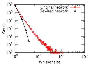
(a) LiveJournal01

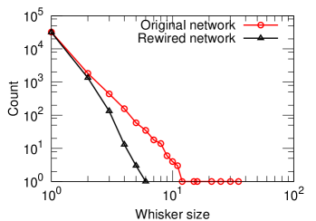
(b) Epinions

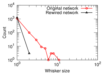
(c) Cit-hep-th

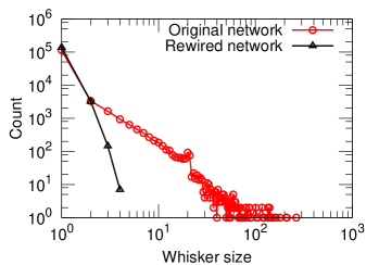
(d) Web-Google

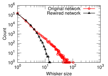
(e) Atp-DBLP

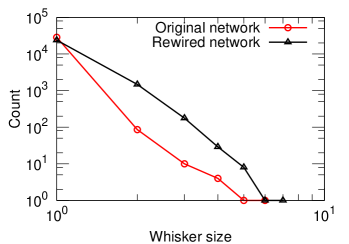
(f) Gnutella-31

Figure 10: Distribution of whisker sizes in the true network and the rewired network (random graph with same degree distribution) for the six networks presented in Figure 6. The ten largest whiskers for the Epinions social network (the full distribution of which is presented here in panel (b)) are presented in Figure 11.

Figure 11 shows the ten largest whiskers of the Epinions social network, the full size distribution of which was plotted in Figure 10(b), and Figure 12 shows the ten largest whiskers of the CA-cond-mat co-authorship network. In these networks, the whiskers have on the order of $10$ nodes, and they are seen to have a rich internal structure. Similar but substantially more complex figures could be generated for networks with larger whiskers. In general, the results we observe are consistent with a knowledge of the fields from which the particular datasets have been drawn. For example, in Web-Google we see very large whiskers. This probably represents a well-connected network between the main categories of a website (e.g., different projects), while the individual project websites have a main index page that then points to the rest of the documents.

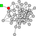
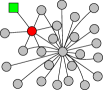
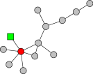
Figure 11: Ten largest whiskers of the Epinions social network. The green square node is the node from the bi-connected core of the network to which the whisker is connected. For visual clarity, the whisker node that connects to the core of the network is displayed in red, and thus it is the edge between the red circle and the green square node that if cut disconnects the whisker from the core. The distribution of whisker sizes and comparison to rewired network is plotted in Figure 10(b).

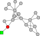
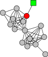
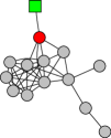
Figure 12: Ten largest whiskers of the CA-cond-mat co-authorship network. The green square node belongs to the network core, and by cutting the edge connecting it with red circular node we separate the community of circles from the rest of the network (depicted as a green square).

The discrepancy between the sizes of the whiskers in the original and the rewired networks gives hints that real networks have much richer structure than that imposed by their heavy-tailed degree distribution. One might ask whether the conclusion from this is that real-world graphs should be thought of as being somewhat like sparse random graphs, since, e.g., both have whiskers, or should be thought of as very different than sparse random graphs, since, e.g., the whiskers have much more internal structure. We will return to this issue in Section 6.

4.3 Bags of whiskers and communities of composed whiskers

Empirically, if one looks at the sets of nodes achieving the minimum in the NCP plot (green Metis+MQI curve), then before the global NCP minimum communities are whiskers and above that size scale they are often unions of disjoint whiskers. To understand the extent to which these whiskers and unions of whiskers are responsible for the “best” conductance sets of different sizes, we have developed the Bag-of-Whiskers Heuristic. We artificially compose “communities” from disconnected whiskers and measure conductance of such clusters. Clearly, interpreting and relating such communities to real-world communities makes little sense as these communities are in fact disconnected.

In more detail, we performed the following experiment: suppose we have a set $W=\{w_{1},w_{2},\ldots\}$ of whiskers. In order to construct the optimal conductance cluster of size $k$, we need to solve the following problem: find a set $C$ of whiskers such that $\sum_{i\in C}N(w_{i})=k$ and $\sum_{i\in C}\frac{d(w_{i})}{|C|}$ is maximized, where $N(w_{i})$ is the number of nodes in $w_{i}$ and $d(w_{i})$ is its total internal degree. We then use a dynamic programming to get an approximate solution to this problem. This way, for each size $k$, we find a cluster that is composed solely from (disconnected) whiskers. Figure 6 as well as Figures 7, 8 and 9 show the results of this heuristic applied to many of our network datasets (blue curve).

There are several observations we can make:

• The largest whisker (denoted with a red square) is the lowest point in nearly all NCP plots. This means that the best conductance community is in a sense trivial as it cuts just a single edge, and in addition that a very simple heuristic can find this set.

• For community size below the critical size of $\approx 100$ nodes (i.e., of size smaller than the largest whisker), the best community in the network is actually a whisker and can be cut by a single edge (blue and red curve overlap).

• For community size larger than the critical size of $\approx 100$, the Bag-of-Whiskers communities have better scores than the internally well-connected communities extracted by Local Spectral (red curve). The shape of this blue curve in that size region depends on the distribution of sizes of whiskers, but in nearly every case it is seen to yield better conductance sets than the Local Spectral Algorithm.

Moreover, the Bag-of-Whiskers Heuristic often agrees, exactly or approximately, with results from Metis+MQI (green curve). In particular, the best conductance sets of a given size are often disconnected, and when they are connected they are often only tenuously connected. Thus, if one only cares about finding good cuts then the best cuts in these large sparse graphs are obtained by composing unrelated disconnected pieces. Intuitively, a compact cluster is internally well and evenly connected. Possible measures for cluster compactness include: cluster connectedness, diameter, conductance of the cut inside the cluster, ratio of conductance of the cut outside versus the cut inside. We discuss this in more detail in Section 5.

4.4 Community profile of networks with no $1$-whiskers

Given the surprisingly significant effect on the community structure of real-world networks that whiskers and unions of disjoint whiskers have, one might wonder whether we see something qualitatively different if we consider a real-world network in which these barely-connected pieces have been removed. To study this, we found all $1$-whiskers and removed them from our networks, using the procedure we described in Section 4.2, i.e., we selected the largest biconnected component for each of our network datasets. This way, we kept only the network core, and we then computed the NCP plots for these modified networks. Figure 13 shows the NCP plots of networks constructed when we remove whiskers (i.e., keep only the network core) for the six networks we studied in detail before.

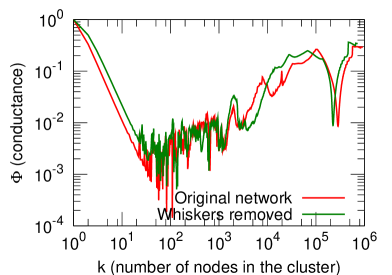
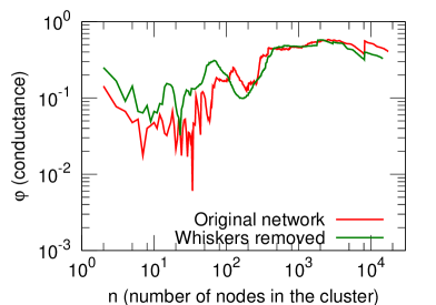
(a) LiveJournal01	(b) Epinions
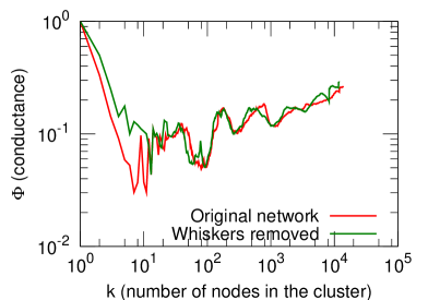
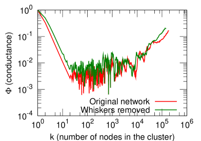
(c) Cit-hep-th	(d) Web-Google
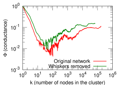
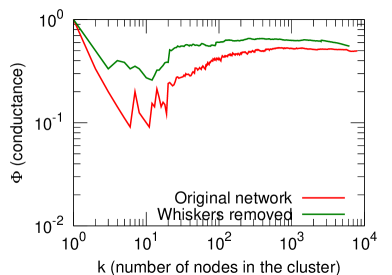
(e) Atp-DBLP	(f) Gnutella-31

Figure 13: [Best viewed in color.] Network community profile plots with (in red) and without (in green) $1$-whiskers, for each of the six networks shown Figure 6. Whiskers were removed as described in the text. In the former case, we plot results for the full network, and in the latter case, we plot results for the largest bi-connected component.

Notice that whisker removal does not change the NCP plot much: the plot shifts slightly upward, but the general trends remain the same. Upon examination, the global minimum occurs with a “2-whisker” that is connected by two edges to the remainder of the graph. Intuitively, the largest biconnected core has a large number of barely connected pieces—connected now by two edges rather than by one edge—and thus the “core” itself has a core-periphery structure. Since the “volume” for these pieces is similar to that for the original whiskers, whereas the “surface area” is a factor of two larger, the conductance value is roughly a factor of two worse. Thus, although we have been discussing $1$-whiskers in this section, one should really view them as the simplest example of weakly-connected pieces that exert a significant effect on the community structure in large real-world networks.

5 Comparison to other algorithms

So far, we have been primarily relying on two graph partitioning algorithms: a Local Spectral Algorithm and Metis+MQI. Next, we want to demonstrate that what we are observing is a true structural property of our network datasets, rather than properties of our algorithms; and we want to use the differences between different approximation algorithms to further highlight structural properties of our network datasets. In this section we discuss several meta-issues related to this, including whether or not our algorithms are sufficiently powerful to recover the true shape of the minimal conductance curves, and whether we should actually be trying to optimize a slightly different measure that combines conductance of the separating cut with the piece compactness.

Recall that we defined the NCP plot to be a curve showing the minimum conductance $\phi$ as a function of piece size $k$. Finding the points on this curve is NP-hard. Any cut that we find will only provide an upper bound on the true minimum at the resulting piece’s size. Given that fact, how confident can we be that the curve of upper bounds that we have computed has the same rising or falling shape as the true curve?

One method for finding out whether any given algorithm is doing a good job of pushing down the upper bounding curve in a non-size-biased way is to compare its curves for numerous graphs with those produced by other algorithms. In such experiments, it is good if the algorithms are very powerful and also independent of each other. We have done extensive experiments along these lines, and our choice of Local Spectral and Metis+MQI as the two algorithms for the main body of this paper was based on the results. In Section 5.1 we mention a few interesting points related to this.

A different method for reducing our uncertainty about the shape of the true curve would be to also compute lower bounds on the curve. Ideally, one would compute a complete curve of tight lower bounds, leaving a thin band between the upper- and lower-bounding curves, which would make the rising or falling shape of the true curve obvious. In Section 5.2 we discuss some experiments with lower bounds. Although we only obtained a few lower bounds rather than a full curve, the results are consistent with our main results obtained from upper-bounding curves.

Finally, in Section 5.3 we will discuss our decision to use the Local Spectral algorithm in addition to Metis+MQI in the main body of the paper, despite the fact that Metis+MQI clearly dominates Local Spectral at the nominal task of finding the lowest possible upper bounding curve for the minimal conductance curve. The reason for this decision is that Local Spectral often returns “nicer” and more “compact” pieces because rather than minimizing conductance alone, it optimizes a slightly different measure that produces a compromise between the conductance of the bounding cut and the “compactness” of the resulting piece.

5.1 Cross-checking between algorithms

As just mentioned, one way to gain some confidence in the upper bounding curves produced by a given algorithm is to compare them with the curves produced by other algorithms that are as strong as possible, and as independent as possible. We have extensively experimented with several variants of the global spectral method, both the usual eigenvector-based embedding on a line, and an SDP-based embedding on a hypersphere, both with the usual hyperplane-sweep rounding method and a fancier flow-based rounding method which includes MQI as the last step. In addition, special post-processing can be done to obtain either connected or disconnected sets. After examining the output of those 8 comparatively expensive algorithms on more than $100$ graphs, we found that our two cheaper main algorithms did miss an occasional cut on an occasional graph, but nothing at all serious enough to change our main conclusions. All of those detailed results are suppressed in this paper.

We have also done experiments with a practical version of the Leighton-Rao algorithm [107, 108], similar to the implementation described in [105] and [106]. These results are especially interesting because the Leighton-Rao algorithm, which is based on multi-commodity flow, provides a completely independent check on Metis, and on Spectral Methods generally, and therefore on our two main algorithms, namely Metis+MQI and Local Spectral. The Leighton-Rao algorithm has two phases. In the first phase, edge congestions are produced by routing a large number of commodities through the network. We adapted our program to optimize conductance (rather than ordinary ratio cut score) by letting the expected demand between a pair of nodes be proportional to the product of their degrees. In the second phase, a rounding algorithm is used to convert edge congestions into actual cuts. Our method was to sweep over node orderings produced by running Prim’s MST algorithm on the congestion graph, starting from a large number of different initial nodes, using a range of different scales to avoid quadratic run time. We used two variations of this method, one that only produces connected sets, and another one that can also produce disconnected sets.

In the second row of Figure 14, we show Leighton-Rao curves for three example graphs. Our standard Local Spectral and Metis+MQI curves are drawn in black, while the Leighton-Rao curves for connected and possibly disconnected sets are drawn in green and magenta respectively. We note that for small to medium scales, the Leighton-Rao curves for connected sets resemble the Local Spectral curves, while the Leighton-Rao curves for possibly disconnected sets resemble the Metis+MQI curves. This is big hint about the structure of the sets produced by Local Spectral and Metis+MQI, that we will discuss further in Section 5.3.

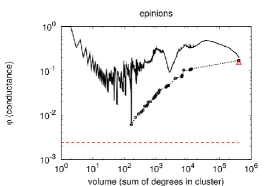
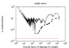
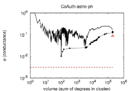
Lower bounds on the conductance of best cut in the network.

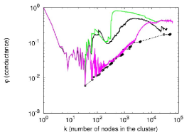
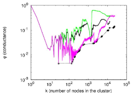
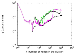
Leighton-Rao: connected clusters (green), disconnected clusters (magenta).

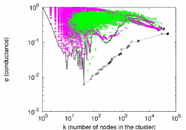
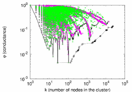
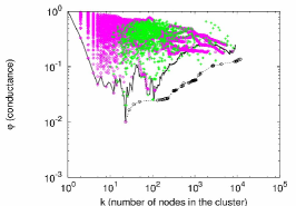
NCP plots obtained by Graclus and Newman’s Dendrogram algorithm.

Figure 14: Result of other algorithms for three networks: Epinions, Email-Enron, and CA-astro-ph. Top row plots (in black) conductance curves as obtained by Local Spectral and Metis+MQI. Top row also shows lower bounds on conductance of any cut (Spectral lower bound, dashed line) and the cut separating the graph in half (SDP lower bound, red triangle). Middle row shows NCP plots for connected (green) and disconnected (magenta) pieces from our implementation of the Leighton-Rao algorithm. Bottom row shows the conductance of some cuts found by Graclus and by Newman’s Dendrogram algorithm. The overall conclusion is that the qualitative shape of the NCP plots is a structural property of large networks and the plot remains practically unchanged regardless of what particular community detection algorithm we use.

At large scales, the Leighton-Rao curves for these example graphs shoot up and become much worse than our standard curves. This is not surprising because expander graphs are known to be the worst case input for the Leighton-Rao approximation guarantee, and we believe that these graphs contain an expander-like core that is necessarily encountered at large scales. We remark that Leighton-Rao does not work poorly at large scales on every kind of graph. (In fact, for large low-dimensional mesh-like graphs, Leighton-Rao is a very cheap and effective method for finding cuts at all scales, while our local spectral method becomes impractically slow at medium to large scales. We will not discuss this point further, except to note that in the main body of the paper we have silently substituted Leighton-Rao curves for local spectral curves for the large road networks and similar graphs.)

We have now covered the main theoretical algorithms that are practical enough to actually run, which are based on spectral embeddings and on multi-commodity flow. Starting with [17], there has been a recent burst of theoretical activity showing that spectral and flow-based ideas, which were already known to have complementary strengths and weaknesses, can in fact be combined to obtain the best ever approximations. At present none of the resulting algorithms are sufficiently practical at the sizes that we require, so they were not included in this study.

Finally, we mention that in addition to the above theoretically-based practical methods for finding low-conductance cuts, there exist a very large number of heuristic graph clustering methods. We have tried a number of them, including Graclus [54] and Newman’s modularity optimizing program (we refer to it as Dendrogram) [80]. Graclus attempts to find a partitioning of a graph into pieces bounded by low-conductance cuts using a kernel k-means algorithm. We ran Graclus repeatedly, asking for $2,3,\dots,i,\dots,i*\sqrt{2},...$ pieces. Then we measured the size and conductance of all of the resulting pieces. Newman’s Dendrogram program constructs a recursive partitioning of a graph (that is, a dendrogram) from the bottom up by repeatedly deleting the surviving edge with the highest betweenness centrality. A flat partitioning could then be obtained by cutting at the level which gives the highest modularity score, but instead of doing that, we measured the size of conductance of every piece defined by a subtree in the dendrogram.

In the bottom row of Figure 14, we present these results as scatterplots. Again our two standard curves are drawn in black. No Graclus or Dendrogram point lies below the Metis+MQI curve. The lower-envelopes of the points are roughly similar to those produced by Local Spectral.

Our main point with these experiments is that the lowest points produced by either Graclus or Dendrogram gradually rise as one moves from small scales to larger scales, so in principle we could have made the same observations about the structure of large social and information networks by running one of those easily downloadable programs instead of the algorithms that we did run. We chose the algorithms we did due to their speed and power, although they may not be as familiar to many readers.

5.2 Lower bounds on cut conductance

As mentioned above, our main arguments are all based on curves which are actually upper bounds on the true minimum conductance curve. To get a better idea of how good those upper bounds are, we also compute some lower bounds. Here we will discuss the spectral lower bound [34] on the conductance of cuts of arbitrary balance, and we will also discuss a related SDP-based lower bound [28] on the conductance of any cut that divides the graph into two pieces of equal volume.

First, we introduce the following notation: $\vec{d}$ is a column vector of the graph’s node degrees; $D$ is a square matrix whose only nonzero entries are the graph’s node degrees on the diagonal; $A$ is the adjacency matrix of $G$; $L=D-A$ is then the non-normalized Laplacian matrix of $G$; 1 is vector of 1’s; and $A\bullet B=trace(A^{T}B)$ is the matrix dot-product operator.

Now, consider the following optimization problem (which is well known to be equivalent to an eigenproblem):

$$\lambda_{G}={\rm min}\left\{\frac{x^{T}Lx}{x^{T}Dx}:x\perp\vec{d},x\neq 0\right\}.$$

Let $\hat{x}$ be a vector achieving the minimum value $\lambda_{G}$. Then $\frac{\lambda_{G}}{2}$ is the spectral lower bound on the conductance of any cut in the graph, regardless of balance, while $\hat{x}$ defines a spectral embedding of the graph on a line, to which rounding algorithms can be applied to obtain actual cuts that can serve as upper bounds at various sizes.

Next, we discuss an SDP-based lower bound on cuts which partition the graph into two sets of exactly equal volume. Consider:

$$\mathcal{C}_{G}={\rm min}\left\{\frac{1}{4}L\bullet Y:diag(Y)={\bf 1},Y\bullet(\vec{d}\,\vec{d}^{\,T})=0,Y\succeq 0\right\},$$

and let $\hat{Y}$ be a matrix achieving the minimum value $\mathcal{C}_{G}$. Then $\mathcal{C}_{G}$ is a lower bound on the weight of any cut with perfect volume balance, and $2\mathcal{C}_{G}/{\rm Vol}(G)$ is a lower bound on the conductance of any cut with perfect volume balance. We briefly mention that since $Y\succeq 0$, we can view $Y$ as a Gram matrix that can be factored can be factored as $RR^{T}$. Then the rows of $R$ are the coordinates of an embedding of the graph on a hypersphere. Again, rounding algorithms can be applied to the embedding to obtain actual cuts that can server as upper bounds.

The spectral and SDP embeddings defined here were the basis for the extensive experiments with global spectral partitioning methods that were alluded to in Section 5.1. However, in this section, it is the lower bounds that concern us. In the top row of Figure 14, we present the spectral and SDP lower bounds for three example graphs. The spectral lower bound, which applies to cuts of any balance, is drawn as a horizontal line which appears near the bottom of each plot. The SDP lower bound, which only applies to cuts separating a specific volume, namely ${\rm Vol}(G)/2$, appears as an upwards-pointing triangle near the right side of the each plot. (Note that plotting this point required us to use volume rather than number of nodes for the x-axis of these three plots.)

Clearly, for these graphs, the lower bound at ${\rm Vol}(G)/2$, is higher than the spectral lower bound which applies at smaller scales. More importantly, the lower bound at ${\rm Vol}(G)/2$, is higher than our upper bounds at many smaller scales, so the true curve must go up, at least at the very end, as one moves from small to large scales.

Take, for example, the top left plot of Figure 14 where in black we plot the conductance curves obtained by our (Local Spectral and Metis+MQI) algorithms. With a red dashed line we also plot the lower bound of best possible cut in the network, and with red triangle we plot the lower bound for the cut that separates the graph in two equal volume parts. Thus, the true conductance curve (which is intractable to compute) lies below black but above red line and red triangle. This also demonstrates that the conductance curve which starts at upper left corner of the NCP plot first goes down and reaches the minimum close to the horizontal dashed line (Spectral lower bound) and then sharply rise and ends up above the red triangle (SDP lower bound). This verifies that our conductance curves and obtained NCP plots are not the artifacts of community detection algorithms we employed.

Finally, in Table 4 we list for about 40 graphs the spectral and SDP lower bounds on overall conductance and on volume-bisecting conductance, and also the ratio between the two. It is interesting to see that for these graphs this ratio of lower bounds does a fairly good job of discriminating between falling-NCP-plot graphs, which have a small ratio, and rising-NCP-plot graphs, which have a large ratio. Small networks (like CollegeFootball, ZacharyKarate and MonksNetwork) have downward NCP plot and a small ratio of the SDP and Spectral lower bounds. On the other hand large networks (e.g., Epinions or Answers-3) that have downward and then upward NCP plot (as in Figure 2(a)) have large ratio of the two lower bounds. This is further evidence that small networks have fundamentally different community structure from large networks and that one has to examine very large networks to observe the gradual absence of communities of size above $\approx 100$ nodes.

	Spectral	SDP	ratio
	lowerbnd	lowerbnd	of
	on $\phi$,	on $\phi$, at	lower
Network	any size.	${\rm Vol}(G)/2$	bnds
CollegeFootball [5]	0.068402	0.091017	1.330624
MonksNetwork [5]	0.069660	0.117117	1.681269
ZacharyKarate [5]	0.066136	0.127625	1.929736
PowerGrid	0.000136	0.000268	1.978484
PoliticalBooks [5]	0.018902	0.038031	2.011991
PoliticalBlogs [5]	0.040720	0.084052	2.064157
RB-Hierarchical [138]	0.011930	0.030335	2.542792
Email-InOut	0.038669	0.113367	2.931752
NetworkScience [5]	0.001513	0.004502	2.974695
As-Oregon	0.012543	0.042976	3.426417
Blog-nat05-6m	0.031604	0.108979	3.448250
Imdb-India	0.009104	0.033318	3.659573
Cit-hep-ph	0.007858	0.029243	3.721553
Bio-Proteins	0.033714	0.126137	3.741358
As-RouteViews	0.018681	0.070462	3.771821
Gnutella-31	0.029946	0.118711	3.964127
Imdb-Japan	0.003327	0.013396	4.026721
Gnutella-30	0.030621	0.124929	4.079853
DolphinsNetwork [5]	0.019762	0.103676	5.246171
As-Newman	0.009681	0.058952	6.089191
AtP-gr-qc	0.000846	0.006040	7.141270
Cit-hep-th	0.009193	0.068880	7.492522
AtP-cond-mat	0.001703	0.013452	7.897650

	Spectral	SDP	ratio
	lowerbnd	lowerbnd	of
	on $\phi$,	on $\phi$, at	lower
Network	any size.	${\rm Vol}(G)/2$	bnds
Gnutella-25	0.014185	0.131032	9.237332
Answers-2	0.009660	0.107422	11.120081
CA-cond-mat	0.003593	0.047064	13.098027
Answers-1	0.011896	0.159251	13.386528
Imdb-France	0.003462	0.048010	13.867591
Answers-5	0.008714	0.124703	14.311255
Imdb-Mexico	0.003893	0.070345	18.067513
CA-gr-qc	0.000934	0.017421	18.659710
AtP-hep-th	0.000514	0.009714	18.899660
AtP-hep-ph	0.000723	0.013770	19.040287
Imdb-WGermany	0.003025	0.065158	21.538867
AtP-astro-ph	0.001183	0.027256	23.036835
CA-hep-th	0.001561	0.041125	26.350412
CA-astro-ph	0.003143	0.086890	27.648094
Imdb-UK	0.001283	0.036572	28.514376
Imdb-Germany	0.000661	0.021017	31.810460
Blog-nat06all	0.002361	0.092908	39.350874
Imdb-Italy	0.000679	0.031954	47.077242
Email-Enron	0.001763	0.089876	50.965424
CA-hep-ph	0.000889	0.052249	58.755927
Epinions	0.002395	0.150242	62.739252
Answers-3	0.002636	0.185340	70.306807
Imdb-Spain	0.000562	0.046327	82.397702

Table 4: Lower bounds on the conductance for our network datasets. Recall that the spectral lower bound applies to any cut, while the SDP lower bound applies to cuts at a specified volume fraction, taken here to be half. See the top row of Figure 14 for plots for three of these networks.

5.3 Local Spectral and Metis+MQI

In this section we discuss our rationale for using Local Spectral in addition to Metis+MQI as one of our two main algorithms for finding sets bounded by low conductance cuts. This choice requires some justification because the NCP plots are intended to show the tightest possible upper bound on the lowest conductance cut for each piece size, while the curve for Local Spectral is generally above that for Metis+MQI.

Our reason for using Local Spectral in addition to Metis+MQI is that Local Spectral returns pieces that are internally “nicer”. For graphs with a rising NCP plot, we have found that many of the low conductance sets returned by Metis+MQI (or Leighton-Rao, or the Bag-of-Whiskers Heuristic) are actually disconnected. Since internally disconnected sets are not very satisfying “communities”, it is natural to wonder about NCP plot-style curves with the additional requirement that pieces must be internally well connected. In Section 5.1, we generated such a curve using Leighton-Rao, and found that the curve corresponding to connected pieces was higher than a curve allowing disconnected sets.

In the top row of Figure 15, we show scatter plots illustrating a similar comparison between the conductance of the cuts bounding connected pieces generated by Local Spectral and by Metis+MQI. Our method for getting connected pieces from Metis+MQI here is simply to separately measure each of the pieces in a disconnected set. The blue points in the figures show the conductance of some cuts found by Local Spectral. The red points show the conductance of some cuts found by Metis+MQI. Apparently, Local Spectral and Metis+MQI find similar pieces at very small scales, but at slightly larger scales a gap opens up between the red cloud and the blue cloud. In other words, at those scales Metis+MQI is finding lower conductance cuts than Local Spectral, even when the pieces must be internally connected.

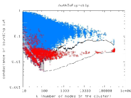
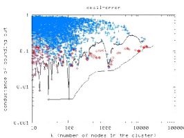
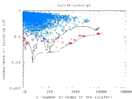
Conductance of connected clusters found by Local Spectral (blue) and Metis+MQI (red)

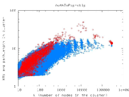
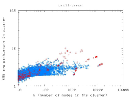
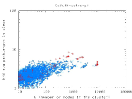
Cluster compactness: average shortest path length

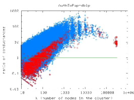
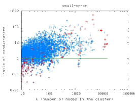
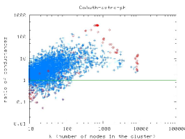
Cluster compactness: external vs. internal conductance

Figure 15: Result of comparing Local Spectral (blue) and Metis+MQI (red) on connected clusters for three networks: AtP-DBLP, Email-Enron, and CA-astro-ph. In the top row, we plot the conductance of the bounding cut. In the middle row, we plot the average shortest path length in the cluster. In the bottom row, we plot the ratio of the external conductance to the internal conductance. Observe that generally Metis+MQI yields better (lower conductance) cuts while Local Spectral yields pieces that are more compact: they have shorter path lengths and internal connectivity.

However, there is still a measurable sense in which the Local Spectral pieces are “nicer” and more “compact,” as shown in the second row of scatter plots in Figure 15. For each of the same pieces for which we plotted a conductance in the top row, we are now plotting the average shortest path length between random node pairs in that piece. In these plots, we see that in the same size range where Metis+MQI is generating clearly lower conductance connected sets, we now see that Local Spectral is generating pieces with clearly shorter internal paths. In other words, the Local Spectral pieces are more “compact”.

Last, in Figure 16, we further illustrate this point with drawings of some example subgraphs. The two subgraphs shown on the left of Figure 16 were found by Local Spectral, while the two subgraphs shown on the right of Figure 16 were found by Metis+MQI. Clearly, these two pairs of subgraphs have a qualitatively different appearance, with the Metis+MQI pieces looking longer and stringier than the Local Spectral pieces. All of these subgraphs contain roughly 500 nodes, which is a bit more than the natural cluster size for that graph, and thus the differences between the algorithms start to show up. In these cases, Local Spectral has grown a cluster out a bit past its natural boundaries (thus the spokes), while Metis+MQI has strung together a couple of different sparsely connected clusters. (We remark that the tendency of Local Spectral to trade off cut quality in favor of piece compactness isn’t just an empirical observation, it is a well understood consequence of the theoretical analysis of spectral partitioning methods.)

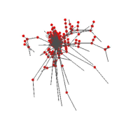
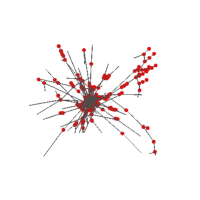
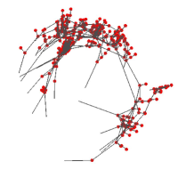
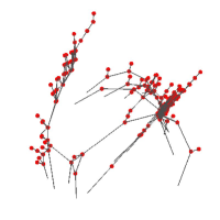
Figure 16: Two examples of “communities” found by the LocalSpectral algorithm (on the left) and two from the Metis+MQI algorithm (on the right). Note that the Local Spectral “communities” are more compact—they are tighter and have smaller diameter since the algorithm has difficulty pushing probability mass down long extended paths—while the Metis+MQI “communities” are more sprawling—they have larger diameter and more diverse internal structure, but better conductance scores. In both cases, we have shown communities with ca. $500$ nodes (many of which overlap at resolution of this figure), i.e., just above the “whisker” size scale.

Finally, in the bottom row of Figure 15 we briefly introduce the topic of internal vs. external cuts, which is something that none of our algorithms are explicitly trying to optimize. These are again scatter plots showing the same set of Local Spectral and Metis+MQI pieces as before, but now the y-axis is external conductance divided by internal conductance. External conductance is the quantity that we usually plot, namely the conductance of the cut which separates the piece from the graph. Internal conductance is the score of a low conductance cut inside the piece (that is, in the induced subgraph on the piece’s nodes). Intuitively, good communities should have small ratios, ideally below 1.0, which would mean that they are well separated from the rest of the network, but that they are internally well-connected. However, the three bottom-row plots show that for these three sample graphs, there are mostly no ratios well below 1.0 except at small sizes. (Of course, any given graph could happen to contain a very distinct piece of any size, and the roughly thousand-node piece in the Email-Enron network is a good example.)

This demonstrates another aspect of our findings: small communities of size below $\approx 100$ nodes are internally compact and well separated from the remainder of the network, whereas larger pieces are so hard to separate that separating them from the network is more expensive than separating them internally.

6 Models for network community structure

In this section, we use results from previous sections to devise a model that explains the shape of NCP plots. In Section 6.1, we examine the NCP plot for a wide range of existing commonly-used network generation models, and we see that none of them reproduces the observed properties, at even a qualitative level. Then, in Section 6.2, we analytically demonstrate that certain aspects of the NCP plot, e.g., the existence of deep cuts at small size scales, can be explained by very sparse random graph models. Then, in Section 6.3, we present a simple toy model to develop intuition about the effect we must reproduce with a realistic generative model. Finally, in Section 6.4, we will combine these and other ideas to describe a Forest Fire graph generation model that reproduces quite well our main observations.

6.1 Community profile plots for commonly-used network generation models

We have studied a wide range of commonly-used network generative models in an effort to reproduce the upward-sloping NCP plots and to understand the structural properties of the real-world networks that are responsible for this phenomenon. In each case, we have experimented with a range of parameters, and in no case have we been able to reproduce our empirical observations, at even a qualitative level. In Figure 17, we summarize these results.

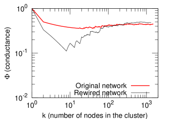
(a) Preferential attachment

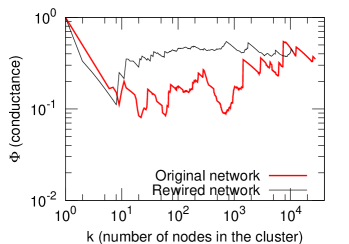
(b) Copying model

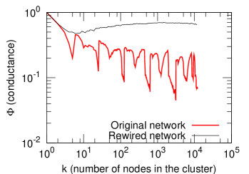
(c) Barabasi Hierarchical

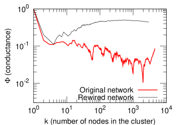
(d) Community guided attachment

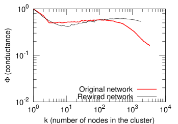
(e) Geometric PA [71]

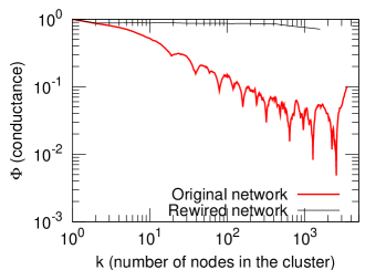
(f) Nested Communities

Figure 17: [Best viewed in color.] Network community profile for networks generated from commonly-used procedures to generate graphs with heavy-tailed degree distributions: (17(a)) Preferential attachment; (17(b)) Copying model; (17(c)) Hierarchical model; (17(d)) Community guided attachment; (17(e)) Geometric preferential attachment; and (17(f)) Nested community model. See the text for details. Red curves plot the results of the Local Spectral Algorithm on the specified network, and black curves plot the results of the Local Spectral Algorithm applied to a randomly rewired version of the same network.

There has been a large body of work subsequent to that of Albert and Barabási [9] on models in which edges are added via a preferential-attachment or rich-gets-richer mechanism [127, 25]. Much of this work aims at reproducing properties of real-world graphs such as heavy-tailed degree distributions [11, 27, 62]. In these preferential attachment models, one typically connects each new node to the existing network by adding exactly $m$ edges to existing nodes with a probability that depends on the current degree of that existing node. Figure 17(a) shows the NCP plot for a $10,000$ node network generated according to the original preferential attachment model [9], where at each time step a node joins the graph and connects to $m=2$ existing nodes. Note that the NCP plot is very shallow and flat (more even than the corresponding rewired graph), and thus the network that is generated is expander-like at all size scales.

A different type of generative model is one in which edges are added via a copying mechanism [102]. In this copying model, a new node joins the network by attaching exactly $m$ edges to existing nodes as follows: the new node first selects uniformly at random a “seed” or “ambassador” node $u$; then, for each of its $m$ edges, with probability $\beta$ the new node links to an existing node chosen randomly, and with probability $1-\beta$ it links to a random neighbor of node $u$. In Figure 17(b), we show the results for a network with $50,000$ nodes, generated with $m=2$ and $\beta=0.05$. Although intuitively the copying model aims to produce communities by linking a new node to neighbors of a existing node, this does not seem to be the right mechanism to reproduce the NCP plot since potential ambassador nodes are all treated similarly and since new nodes always create the same number of edges.

Next, in Figure 17(c), we consider an example of a network that was designed to have a recursively hierarchical community structure [139, 138]. In this model, we start with a $5$-node square-like structure with a central node, and then recursively expand the square and link it to the middle node of the network. This network has power-law degree distribution, and clustering coefficient that decays as in a characteristic manner [138]. In this case, however, the NCP plot is sloping downwards. The local dips in the plot correspond to multiples of the size of the basic module of the graph. Although the model generates links such that nodes that are farther apart in the hierarchy link less frequently, the NCP plot clearly indicates that in aggregate larger communities are easily separated than smaller communities.

A different way to generate power-law degree distributions is the Community Guided Attachment model [112]. Here we decompose the nodes of a graph into a nested groups of nodes, such that the difficulty of forming links between nodes in different groups increases exponentially with the distance in the community hierarchy. Graphs generated by this principle have both power-law degree distributions and they also obey the Densification Power Law [112, 113]. As Figure 17(d) shows, though, the NCP plot is sloping downward. Qualitatively this plot from CGA is very similar to the plot of the recursive hierarchical construction in Figure 17(c), which is not surprising given the similarities of the models.

Figure 17(e) shows the NCP plot for a geometric preferential attachment model [71, 72]. This model aims to achieve a heavy-tailed degree distribution as well edge locality, and it does so by making the connection probabilities depend both on the two-dimensional geometry and on the preferential attachment scheme. As we see, the effect of the underlying geometry eventually dominates the NCP plot since the best bi-partitions are fairly well-balanced [71]. Intuitively, geometric preferential attachment graphs look locally expander-like, but at larger size scales the the union of such small expander graphs behaves like a geometric mesh. We also experimented with the small-world model by Watts and Strogatz [156], in which the NCP plot in some sense behaves exactly the opposite (plot not shown): first the NCP plot decreases, and then it flattens out. Intuitively, a small-world network looks locally like a mesh, but when one reaches larger size scales, the randomly rewired edges start to appear and the graph looks like an expander.

Finally, we explored in more detail networks with explicitly planted community structure. For example, we started with $10$ isolated communities generated using the $G_{n,p}$ model, and then we generated a random binary tree. For each internal node at height $h$ we link the nodes in both sides of the tree with probability $p^{h}$, for a probability parameter $p$. This and other related networks gives a graph of nested communities resembling the hierarchical clustering algorithm of Newman and Girvan [132]. We see, however, from Figure 17(f) that the NCP plot slopes steadily downward, and furthermore we observe that dips correspond to the cuts that separate the communities.

These experiments demonstrate that hierarchically nested networks and networks with underlying geometric or expander like structure exhibit very different NCP plots than observed in real networks. So the question still remains: what causes NCP plot to decrease and then start to increase?

6.2 Very sparse random graphs have very unbalanced deep cuts

In this section, we will analyze a very simple random graph model which reproduces relatively deep cuts at small size scales and which has a NCP plot that then flattens out. Understanding why this happens will be instructive as a baseline for understanding the community properties we have observed in our real-world networks.

Here we work with the random graph model with given expected degrees, as described by Chung and Lu [42, 40, 44, 39, 41, 45, 46, 43]. Let $n$, the number of nodes in the graph, and a vector ${\bf{w}}=(w_{1},\ldots,w_{n})$, which will be the expected degree sequence vector (where we will assume that $\max_{i}w_{i}^{2}<\sum_{k}w_{k}$), be given. Then, in this random graph model, an edge $e_{ij}$ between nodes $i$ and $j$ is added, independently, with probability $p_{ij}=w_{i}w_{j}/\sum_{k}w_{k}$. Thus, $P(e_{ij}=1)=p_{ij}$ and $P(e_{ij}=0)=1-p_{ij}$. We use $G(\bf{w})$ to denote a random graph generated in this manner. (Note that this model is different than the so-called “configuration model” in which the degree distribution is exactly specified and which was studied by Molloy and Reed [124, 125] and also Aiello, Chung, and Lu [7, 8]. This model is also different than generative models such as preferential attachment models [9, 127, 25] or models based on optimization [57, 58, 61], although common to all of these generative models is that they attempt to reproduce empirically-observed power-law behavior [11, 62, 27, 129, 50].)

In this random graph model, the expected average degree is $w_{av}=\frac{1}{n}\sum_{i=1}^{n}w_{i}$ and the expected second-order average degree is $\tilde{w}=\sum_{i=1}^{n}w_{i}^{2}/\sum_{k}w_{k}$. Let $w_{G}=\sum_{i}w_{i}$ denote the expected total degree. Given a subset $S$ of nodes, we define the volume of $S$ to be $w_{S}=\sum_{v\in S}w_{v}$ and we say that $S$ is $c$-giant if its volume is at least $cw_{G}$, for some constant $c>0$. We will denote the actual degrees of the graph $G$ by $\{d_{1},d_{2},\ldots,d_{n}\}$, and will define $d(S)$ to be the sum of the actual degrees of the vertices in $S$. Clearly, by linearity of expectation, for any subset $S$, $E(d(S))=w_{S}$.

The special case of the $G(\bf{w})$ model in which $\bf{w}$ has a power law distribution is of interest to us here. (The other interesting special case, in which all the expected degrees $w_{i}$ are equal to $np$, for some $p\in[0,1]$, corresponds to the classical Erdös-Renyi $G_{np}$ random graph model [24].) Given the number of nodes $n$, the power-law exponent $\beta$, and the parameters $w$ and $w_{\max}$, Chung and Lu [42] give the degree sequence for a power-law graph:

$$w_{i}=ci^{-1/(\beta-1)}\mbox{ for }i\mbox{ s.t. }i_{0}\leq i<n+i_{0},$$ (10)

where, for the sake of consistency with their notation, we index the nodes from $i_{0}$ to $n+i_{0}-1$, and where $c=c(\beta,w,n)$ and $i_{0}=i_{0}(\beta,w,n,w_{\max})$ are as follows:

$$c=\alpha wn^{1/(\beta-1)}\mbox{ and }i_{0}=n\left(\alpha\frac{w}{w_{\max}}\right)^{\beta-1},$$ (11)

where we have defined $\alpha=\frac{\beta-2}{\beta-1}$. It is easy to verify that: $w_{\max}=\max_{i}w_{i}$ is the maximum expected degree; the average expected degree is given by $w_{av}=\frac{1}{n}\sum_{i=1}^{n}w_{i}=w(1+o(1))$; the minimum expected degree is given by $w_{\min}=\min_{i}w_{i}=w\alpha(1-o(1))$; and the number of vertices that have expected degree in the range $(k-1,k]$ is proportional to $k^{-\beta}$.

The following theorem characterizes the shape of the NCP plot for this $G(\bf{w})$ model when the degree distribution follows Equation (10), with $\beta\in(2,3)$. The theorem makes two complementary claims. First, there exists at least one (small but moderately deep) cut in the graph of size $\Theta(\log n)$ and conductance $\Theta(\frac{1}{\log n})$. Second, for some constants $c^{\prime}$ and $\epsilon$, there are no cuts in the graph of size greater than $c^{\prime}\log n$ having conductance less than $\epsilon$. That is, this model has clusters of of logarithmic size with logarithmically deep cuts, and once we get beyond this size scale there do not exist any such deep cuts.

Theorem 1

Consider the random power-law graph model $G(\bf{w})$, where $\bf{w}$ is given by Equation (10), where $w>5.88$, and the power-law exponent $\beta$ satisfies $2<\beta<3$. Then, then with probability $1-o(1)$:

1. There exists a cut of size $\Theta(\log n)$ whose conductance is $\Theta\left(\frac{1}{\log n}\right)$.

2. There exists $c^{\prime},\epsilon>0$ such that there are no sets of size larger than $c^{\prime}\log n$ having conductance smaller than $\epsilon$.

Proof: Combine the results of Lemma 1 and Lemma 3.  

The two claims of Theorem 1 are illustrated in Figure 18(a). Note that when $w\geq\frac{4}{e}$ and $\beta\in(2,3)$ then a typical graph in this model is not fully connected but does have a giant component [42]. (The well-studied $G_{n,p}$ random graph model [24] has a similar regime when $p\in(1/n,\log n/n)$, as will be discussed in Section 7.4.)

In addition, under certain conditions on the average degree and second order average degree, the average distance between nodes is in $O\left(\log\log n\right)$ and yet the diameter of the graph is $\Theta\left(\log n\right)$. Thus, in this case, the graph has an “octopus” structure, with a subgraph containing $n^{c/(\log\log n)}$ nodes constituting a deep core of the graph. The diameter of this core is $O(\log\log n)$ and almost all vertices are at a distance of $O(\log\log n)$ from this core. However, the pairwise average distance of nodes in the entire graph is $O(\log n/\log\tilde{w})$. A schematic picture of the $G(\bf{w})$ model when $\beta\in(2,3)$ is presented in Figure 18(b).

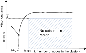
(a) NCP plot suggested by our main theorem

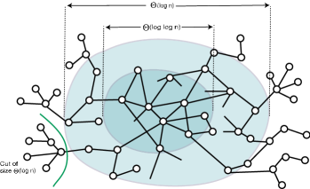
(b) Structure of $G(\bf{w})$ model

Figure 18: The $G(\bf{w})$ model in the sparse $\beta\in(2,3)$ parameter regime. (a) Network community profile plot, as suggested by our main theorem. (b) Caricature of network structure.

Our first lemma claims that for the $G(\bf{w})$ model, if the degree distribution $\bf{w}$ follows the above power-law, then there exists a moderately large cut with small conductance. In order to prove the existence of a cut of size $\Theta(\log n)$ and conductance $\Theta(\frac{1}{\log n})$, it is sufficient to concentrate on the existence of whiskers that are large enough. In particular, to prove the following lemma, we compute the probability that there exists a cut of both volume and size $\Theta(\log n)$ and cut-size $1$. (Note that although we formally state the lemma in terms of the power-law random graph model, the proof will show that the main claim holds for a more general representation of the heavy-tailed degree distribution.)

Lemma 1

For the $G(\bf{w})$ model, where $w$ follows a power-law degree distribution with $2<\beta<3$ then, with probability $1-o(1)$ there exists a set of size $\Theta(\log n)$ with conductance $\Theta(\frac{1}{\log n})$.

Proof: Let $S$ be a subset with the following description. $S=\{v_{0},v_{1},\ldots,v_{k}\}$, where $k=c_{1}\log n$. Let $w_{i}$ denote the degree of $v_{i}$. We have that $w_{0}\in[c_{2}\log n,2c_{2}\log n]$ and $w_{i}\leq w$ for all $i>0$. Thus the expected volume of $S$ is $w_{S}\in[(2\alpha wc_{2}+c_{1})\log n,(2\alpha wc_{2}+c_{1})\log n]$, and the size of $S$ is $c_{1}\log n+1$. Note that the expected volume of the graph can be computed as $w_{G}=wn$, and hence $\rho=\frac{1}{w_{G}}=\frac{1}{wn}$.

Now, let $n_{1}$ denote the number of vertices of expected degree at most $2\alpha w$. By simple calculation, $n_{1}\geq n/2$. The number of possible choices for the vertex $v_{0}$ can be computed as follows. Let $B$ be the set of vertices having degree greater than $2\alpha wc_{2}\log n$ and $A$ be the set of vertices with degree at most $2\alpha wc_{2}\log n$. Then the number of nodes with degree in $[c_{2}\log n,2c_{2}\log n]$ is given by the size of $V\setminus(A\cup B)$ which is

$$\alpha w\left(\frac{n}{c_{2}\log n}\right)^{\beta-1}-\alpha w\left(\frac{n}{2c_{2}\log n}\right)^{\beta-1}\geq\alpha w\left(\frac{n}{c_{2}\log n}\right)^{\beta-1},$$

since $\beta>2$. Thus the number of possible such subsets $S$ is given by the number of choices for $v_{0}$ times the number of possible choices for the nodes $v-1,\ldots,v_{k}$. Thus, the number $N$ of possible such subsets $S$ is at least

$$N={n_{1}\choose c_{1}\log n}\times\alpha\left(\frac{n}{2c_{2}\log n}\right)^{\beta-1}.$$

We say that $S$ is good if, after instantiating all the edges, $S$ has a star of size $c_{1}\log n$ centered at $v_{0}$, and $v_{0}$ is connected to $\bar{S}$ by exactly one edge, and none of the other vertices in $S$ have any edge to $\bar{S}$. The probability that a particular set $S$ is good is the product of the following terms: the probability $p_{1}$ that there is star of size $c_{1}\log n$ with $v_{0}$ at the center, the probability $p_{2}$ that none of the nodes $v_{1},\ldots,v_{k}$ link to any nodes in $\bar{S}$, and the probability $p_{3}$ that $v_{0}$ connects to $\bar{S}$ using exactly one edge. We now calculate the three probabilities as follows. First,

$$p_{1}=\prod_{i\in[1\ldots k]}w_{0}w_{i}\rho\geq(w_{0}\alpha w\rho)^{c_{1}\log n},$$

since each $w_{i}\geq w_{\min}\geq\alpha w$. Next,

$$p_{2}=\prod_{i=1,\ldots k}\prod_{j\notin S}(1-w_{j}\rho)\geq\prod_{i=1,\ldots k}\prod_{j\notin S}e^{-w_{i}\rho/2}=e^{-(c_{1}\rho 2\alpha ww_{\bar{S}}\log n)/2},$$

obtained by using $1-x\geq e^{-x/2}$ for $0<x<1$, and $w_{i}\leq 2\alpha w$ for $i\in S,i>1$. Finally, we get $p_{3}$ as follows. First note

$$p_{3}= \;\sum_{j\in\bar{S}}w_{0}w_{j}\rho\prod_{k\neq j,k\in\bar{S}}(1-w_{k}w_{0}\rho)$$

$$\geq \;\sum_{j\in\bar{S}}w_{0}w_{j}\rho e^{-(w_{\bar{S}}\;-w_{j})w_{0}\rho/2}$$

$$= \;w_{0}\rho e^{-w_{\bar{S}}w_{0}\rho/2}(\sum_{j\in\bar{S}}w_{j}e^{w_{j}w_{0}\rho/2}).$$

Then, since $w_{j}w_{0}\rho\ll 1$ and since $e^{x}\geq 1+x$, we have that

$$p_{3}\geq \;w_{0}\rho e^{-w_{\bar{S}}w_{0}\rho/2}(\sum_{j\in\bar{S}}w_{j}(1+\frac{w_{j}w_{0}\rho}{2}))$$

$$\geq \;w_{0}\rho e^{-w_{\bar{S}}w_{0}\rho/2}(w_{\bar{S}}+w_{0}\rho\tilde{w}_{\bar{S}}/2),$$

where $\tilde{w}_{\bar{S}}=\sum_{j\in\bar{S}}w_{j}^{2}$. So the final probability of goodness of $S$ is

$$p=p_{1}\times p_{2}\times p_{3} \geq (w_{0}\alpha w\rho)^{c_{1}\log n}\times e^{-(c_{1}\rho 2\alpha ww_{\bar{S}}\log n)/2}\times w_{0}\rho e^{-w_{\bar{S}}w_{0}\rho/2}(w_{\bar{S}}+w_{0}\rho\tilde{w}_{\bar{S}}/2)$$

$$= (w_{0}\alpha w\rho)^{c_{1}\log n}\times e^{-(c_{1}\gamma 2\alpha w\log n)}\times w_{0}\rho e^{-\gamma w_{0}}(w_{\bar{S}}+w_{0}\rho\tilde{w}_{\bar{S}}/2),$$

using $\gamma=\rho w_{\bar{S}}/2$. So the expected number of such good subsets $S$ is

$$Np \geq{n_{1}\choose c_{1}\log n}\times\alpha w\left(\frac{n}{2c_{2}\log n}\right)^{\beta-1}\times(w_{0}\alpha w\rho)^{c_{1}\log n}\times e^{-(c_{1}\gamma 2\alpha w\log n)}\times w_{0}\rho e^{-\gamma w_{0}}(w_{\bar{S}}+w_{0}\rho\tilde{w}_{\bar{S}}/2)$$

$$\geq\left(\frac{n_{1}}{c_{1}\log n}\right)^{c_{1}\log n}\times\frac{\alpha wn^{\beta-1}}{(2c_{2}\log n)^{\beta-1}}\times(w_{0}\alpha w\rho)^{c_{1}\log n}\times e^{-(c_{1}\gamma 2\alpha w\log n)}\times w_{0}\rho e^{-\gamma w_{0}}\times nw/2,$$

using Stirling’s formula and the fact that $w_{\bar{S}}\geq nw/2$. Using the value of $n_{1}$ and since $nw\rho=1$,

$$Np \geq\left(\frac{n}{2c_{1}\log n}\right)^{c_{1}\log n}\times\frac{\alpha wn^{\beta-1}}{(2c_{2}\log n)^{\beta-1}}\times(w_{0}\alpha w\rho)^{c_{1}\log n}\times e^{-(c_{1}\gamma 2\alpha w\log n)}\times e^{-\gamma w_{0}}\times w_{0}/2$$

$$\geq\left(\frac{w_{0}\alpha}{2c_{1}\log n}\right)^{c_{1}\log n}\times\frac{\alpha wn^{\beta-1}}{(2c_{2}\log n)^{\beta-1}}\times(w_{0}\alpha w\rho)^{c_{1}\log n}\times e^{-(c_{1}\gamma 2\alpha w\log n)}\times e^{-\gamma w_{0}}\times w_{0}/2.$$

Using $w_{0}\geq c_{2}\log n$, we have that have that

$$Np \geq\left(\frac{c_{2}\alpha}{2c_{1}}\right)^{c_{1}\log n}\times\frac{\alpha wn^{\beta-1}}{2(2c_{2}\log n)^{\beta-2}}\times e^{-(c_{1}\gamma 2\alpha w\log n)}\times e^{-\gamma w_{0}}$$

$$\geq e^{\Theta\log n}\times\frac{\alpha w}{2(2c_{2}\log n)^{\beta-2}},$$

where $\Theta=c_{1}\log(\frac{c_{2}\alpha}{2c_{1}})+(\beta-1)-\gamma\alpha wc_{1}-2\gamma c_{2}$. Note that for $2<\beta<3$, we have that $0<\alpha<\frac{1}{2}$. Also, $\gamma=\frac{1}{2}-o(1)$. Thus, choosing $c_{2}=2ec_{1}/\alpha$ and $c_{1}=\frac{\beta-2}{2\gamma\alpha w+4\gamma e/\alpha-1}$, we get $\Theta=1$. So,

$$Np \geq e^{\log n}\times\frac{\alpha w}{2(2c_{2}\log n)^{\beta-2}}=\Omega(\log n)$$

Then, the probability is a particular set $S$ is good is $p\geq\Omega\left(\frac{(\log n)}{N}\right)$. Hence the probability of getting a good set is

$$1-(1-p)^{N}\geq 1-\left(1-\Omega\left(\frac{(\log n)^{\beta-2}}{N}\right)\right)^{N}\geq 1-o(1)$$

 

We next state the well-known Chernoff bound [42], which we will use below.

Lemma 2

Let $X=\sum_{i}X_{i}$ where the $X_{i}$ are independent random variables with $X_{i}\geq-M$. Define $\|X\|^{2}=\sum_{i}{\mathbf{E}}(X_{i}^{2})$. Then,

$${\mathbf{Pr}}(X\geq{\mathbf{E}}(X)-\lambda)\leq\exp\left(-\frac{\lambda^{2}}{2(\|X\|^{2}+M\lambda/3)}\right).$$ (12)

Finally, we show that there are no deep cuts with size greater than $\Theta(\log n)$. To state this lemma, define a connected set $S$ to be $\epsilon$-deficit set if it has actual volume $d(S)\leq\frac{1}{2}d(G)$ and if the conductance of the cut $(S,\bar{S})$ is at most $\epsilon$, i.e., if the number of edges leaving $S$ is at most $\epsilon d(S)$.

Lemma 3

For the $G(\bf{w})$ model, where $w$ follows a power-law degree distribution with $2<\beta<3$, if the average degree $w$ satisfies $w\geq 5.88$, then with probability $1-o(1)$ there exists constants $c^{\prime},\epsilon$ such that there is no $\epsilon$-deficit set of size more than $c^{\prime}\log n$.

Proof: Let $e(S,\bar{S})$ denote the actual number of edges between $S$ and $\bar{S}$. First we compute the probability that a given set $S$ is $\epsilon$-deficit, that is, $S$ satisfies $e(S,\bar{S})<\epsilon d(S)$. Let $\delta=\frac{2\epsilon}{1-\epsilon}$. For our case, define the variables $X_{(i,j)}=e_{ij}$ for $(i,j)\in(S,\bar{S})$ and $X_{(i,j)}=-\delta e_{ij}$ for $(i,j)\in(S,S)$. Then the sum $X=\sum X_{(i,j)}=\sum_{(i,j)\in(S,\bar{S})}e_{ij}-\delta\sum_{(i,j)\in(S,\bar{S})}e_{ij}$. Note that $e(S,\bar{S})<\epsilon d(S)\iff X\leq 0$. Using the fact that ${\mathbf{E}}(e_{ij})=w_{i}w_{j}\rho$, we have $\|X\|^{2}=\sum{\mathbf{E}}(X_{ij}^{2})=w_{S}w_{\bar{S}}\rho+\delta^{2}w_{S}^{2}\rho$. Furthermore, exploiting the fact that each $X_{i}\geq-\delta$, we get that

$${\mathbf{Pr}}(X\leq 0) = {\mathbf{Pr}}(X\leq{\mathbf{E}}(X)-{\mathbf{E}}(X))$$

$$\leq \exp\left(-\frac{{\mathbf{E}}(X)^{2}}{2(\|X\|^{2}+\delta{\mathbf{E}}(X)/3)}\right)$$

$$= \exp\left(-\frac{\rho^{2}w_{S}^{2}(w_{\bar{S}}-\delta w_{S})^{2}}{2(w_{S}\rho(w_{\bar{S}}+\delta^{2}w_{S})+\delta w_{S}\rho(w_{\bar{S}}-\delta w_{S})/3)}\right).$$

Canceling $\rho w_{S}$ from both numerator and denominator,

$${\mathbf{Pr}}(X\leq 0) \leq \exp\left(-\frac{\rho w_{S}(w_{\bar{S}}-\delta w_{S})^{2}}{2(w_{\bar{S}}+\delta^{2}w_{S}+\delta w_{\bar{S}}/3-\delta^{2}w_{S}/3)}\right)$$

$$\leq \exp\left(-\frac{\rho w_{S}(w_{\bar{S}}-\delta w_{S})^{2}}{2(1+\delta/3+2\delta^{2}/3)w_{\bar{S}}}\right)\leq\exp\left(-\frac{\rho w_{S}w_{\bar{S}}(1-2\delta w_{S}/w_{\bar{S}})}{2(1+\delta/3+2\delta^{2}/3)}\right)$$

$$\leq \exp\left(-\frac{\rho w_{S}w_{\bar{S}}(1-2\delta)}{2(1+\delta/3+2\delta^{2}/3)}\right)\leq\exp\left(-\rho w_{S}w_{\bar{S}}A_{\delta}/2\right),$$

where $A_{\delta}=\frac{1-2\delta}{(1+2\delta/3+2\delta^{2}/3)}$. So this bounds the probability that a particular set $S$ of size $k$ is $\epsilon$-deficit. We will bound the expected number of such $\epsilon$-deficit subsets of size $k$. First, let $N_{k,\epsilon,\gamma}$ denote the expected number of $\epsilon$-deficit sets of size $k$ that have expected volume $w_{S}\leq\gamma w_{G}$. By linearity of expectation,

$$N_{k,\epsilon,\gamma} \leq \sum_{\stackrel{{\scriptstyle S:|S|=k}}{{w_{S}\leq\gamma w_{G}}}}w_{i_{1}}\ldots w_{i_{k}}w_{S}^{k-2}\rho^{k-1}\exp\left(-\rho w_{S}w_{\bar{S}}A_{\delta}/2\right)$$

$$\leq \sum_{\stackrel{{\scriptstyle S:|S|=k}}{{w_{S}\leq\gamma w_{G}}}}\frac{w_{S}^{2k-2}}{k^{k}}\rho^{k-1}\exp(\left(-w_{S}(1-\gamma)A_{\delta}\right)),$$

where we used the fact that $\gamma=\rho w_{\bar{S}}/2$ and also the AM-GM inequality to say that $\prod_{i\in S}w_{i}\leq\left(\frac{\sum_{i\in S}w_{i}}{k}\right)^{k}$. Now, $F(x)=x^{2k-2}e^{-xA_{\delta}(1-\gamma)}$ is maximized at $x=\frac{2k-2}{A_{\delta}(1-\gamma)}$. Thus, the above sum is maximized when $w_{S}=\frac{2k-2}{A_{\delta}(1-\gamma)}$. Hence,

$$N_{k,\epsilon,\gamma} \leq \frac{n^{k}}{k!}\frac{\rho^{k-1}}{k^{k}}\frac{2^{(2k-2)}\cdot(k-1)^{(2k-2)}}{(A_{\delta}(1-\gamma))^{(2k-2)}}\exp(-2k+2)$$

$$\leq \frac{(n\rho)^{k}}{\rho\sqrt{k}(k/e)^{k}}\frac{1}{k^{k}}\frac{2^{(2k-2)}\cdot(k-1)^{(2k-2)}}{(A_{\delta}(1-\gamma))^{(2k-2)}}\exp(-2k+2).$$

Using $(1-\frac{1}{k})^{2k}\leq e^{-2}$, it follows that

$$N_{k,\epsilon,\gamma} \leq \frac{1}{4e\sqrt{k}(k-1)^{2}}\left(\frac{4}{ewA_{\delta}^{2}(1-\gamma)^{2}}\right)^{k}.$$

We would like $\sum_{k=c\log n}^{cn}N_{k,\epsilon,\gamma}$ to be $o(1)$, for which we need

$$\frac{4}{ewA_{\delta}^{2}(1-\gamma)^{2}}<1,$$

which gives a bound on average degree:

$$w\geq\frac{4}{A_{\delta}^{2}(1-\gamma)^{2}e}.$$

For sets of volume $w_{S}\geq\gamma w_{G}$, we have the following. From the double-sided Chernoff bound, for any fixed set $S$,

$$|w_{S}-d(S)|\leq\lambda\mbox{ with probability }1-2\exp\left(-\frac{\lambda^{2}}{2(w_{S}+\lambda/3)}\right).$$

So if $\lambda=\sqrt{w_{S}}\log n$, we have the above statement with probability $1-2\exp(-3\log^{2}n/8)$. Similarly,

$$|e(S,\bar{S})-{\mathbf{E}}(e(S,\bar{S}))|\leq\lambda\mbox{ with probability }1-2\exp\left(-\frac{\lambda^{2}}{2(\rho w_{S}w_{\bar{S}}+\lambda/3)}\right).$$

By having $\lambda=\sqrt{\rho w_{S}w_{\bar{S}}}\log n$ the above probability becomes $1-2\exp(-3\log^{2}n/8)$. Now, if both these events occur, then the conductance of the set $S$ is at least $1/3$. So the only way we can get an $\epsilon$-deficit set is at by having one of these conditions to be invalid. The total number of sets of expected volume $\gamma w_{G}$ is bounded by $w_{G}\choose\gamma w_{G}$. So, the expected number of $\epsilon$-deficit sets of volume at least $\gamma w_{G}$ is bounded by

$$\sum_{\gamma\leq\theta\leq 1/2}{w_{G}\choose\theta w_{G}}4\exp(-3\log^{2}n/8)\leq\int_{\gamma\leq\theta\leq 1/2}\frac{1}{\sqrt{\theta w_{G}}}\left(\frac{1}{\theta}\right)^{\theta w_{G}}4\exp(-3\log^{2}n/8)\leq o(1).$$

Thus, putting the two bounds together, the expected number of $\epsilon$-deficit sets of size greater that $c\log n$ is at most $o(1)$. Thus with probability $1-o(1)$ there does not exist an $\epsilon$-deficit set of size greater than $c\log n$.  

6.3 An intuitive toy model for generating an upward-sloping NCP plot

We have seen that commonly-studied models, including preferential attachment models, copying models, simple hierarchical models, and models in which there is an underlying mesh-like or manifold-like geometry are not the right way to think out the community structure of large social and information networks. We have also seen that the extreme sparsity of the networks, coupled with randomness, can be responsible for the deep cuts at small scales.

To build intuition as to what the gradually increasing NCP plot might mean, consider Figure 19. This is a toy example of a network construction in which the NCP plot has a deep dip at a small size scale and then steadily increases. The network shown in Figure 19(a) is an infinite tree that has two parts. The top part, a subtree (with one node in this example, but more generally consisting of $n_{T}$ nodes) is indicative of the whiskers, or the “small scale” structure of the graph. The remaining tree has the property that the number of children increases monotonically with the level of the node. This property is indicative of the fact that as the size of a cluster grows, the number of neighbors that it has also increases. The key insight in this construction is that the best conductance cuts first cut at the top of the growing tree and then gradually work their way “down” the tree, starting with the small subtrees and moving gradually down the levels, as depicted in Figure 19(a).

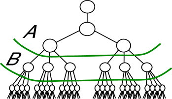
(a) A toy network model $\ldots$

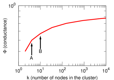
(b) $\ldots$ and its community profile plot.

Figure 19: Schematic picture of the properties of a network responsible for the upward-sloping community profile plot. (a) This toy model is designed so that the optimal conductance cuts are achieved by cutting nodes from the top of the tree. (b) The minimum of the NCP plot is achieved by cutting the single top node, and then larger and larger cuts have gradually worse and worse conductance values.

Thus, intuitively, one can think of small well-separated communities—those below the $n_{T}$ size scale that consist of subsets of the small trees—starting to grow, and as they pass the $n_{T}$ size scale and become bigger and bigger, they blend in more and more with the central part of the network, which (since it exhibits certain expander-like properties) does not have particularly well-defined communities. Note (more generally) that if there are $n_{T}$ nodes in the small tree at the top of the graph, then the dip in the NCP plot in Figure 19(b) is of depth $2/(n_{T}+1)$. In particular, if $n_{T}=\Theta(\log n)$ then the depth of this cut is $\Theta(1/\log n)$.

Intuitively, the NCP plot increases since the “cost” per edge for every additional edge inside a cluster increases with the size of the cluster. For example, in cut $A$ in Figure 19(a), the “price” for having $3$ internal edges is to cut $6$ edges, i.e., $2$ edges cut per edge inside. To expand the cluster by just a single edge, one has to move one level down in the tree (toward the cut $B$) where now the price for a single edge is $4$ edges, and so on.

6.4 A more realistic model of network community structure

The question arises now as to whether we can find a simple generative model that can explain both the existence of small well-separated whisker-like clusters and also an expander-like core whose best clusters get gradually worse as the purported communities increase in size. Intuitively, a satisfactory network generation model must successfully take into account the following two mechanisms:

• The model should produce a relatively large number of relatively small—but still large when compared to random graphs—well connected and distinct whisker-like communities. (This should reproduce the downward part of the community profile plot and the minimum at small size scales.)

• The model should produce a large expander-like core, which may be thought of as consisting of intermingled communities, perhaps growing out from the whisker-like communities, the boundaries of which get less and less well-defined as the communities get larger and larger and as they gradually blend in with rest of the network. (This should reproduce the gradual upward sloping part of the community profile plot.)

The so-called Forest Fire Model [112, 113] captures exactly these two competing phenomena. The Forest Fire Model is a model of graph generation (that generates directed graphs—an effect we will ignore) in which new edges are added via a recursive “burning” mechanism in an epidemic-like fashion. Since the details of the recursive burning process are critical for the model’s success, we explain it in some detail.

To describe the Forest Fire Model of [112, 113], let us fix two parameters, a forward burning probability $p_{f}$ and a backward burning probability $p_{r}$. We start the entire process with a single node, and at each time step $t>1$, we consider a new node $v$ that joins the graph $G_{t}$ constructed thus far. The node $v$ forms out-links to nodes in $G_{t}$ as follows:

• Node $v$ first choose a node $w$, which we will refer to as a “seed” node or an “ambassador” node, uniformly at random and forms a link to $w$.

• Node $v$ selects $x$ out-links and $y$ in-links of $w$ that have not yet been visited. ($x$ and $y$ are two geometrically distributed random numbers with means $p_{f}/(1-p_{f})$ and $p_{r}/(1-p_{r})$, respectively. If not enough in-links or out-links are available, then $v$ selects as many as possible.) Let $w_{1},w_{2},\ldots,w_{x+y}$ denote the nodes at the other ends of these selected links.

• Node $v$ forms out-links to $w_{1},w_{2},\ldots,w_{x+y}$, and then applied step (ii) recursively to each of the $w_{1},w_{2},\ldots,w_{x+y}$, except that nodes cannot be visited a second time during the process.

Thus, burning of links in the Forest Fire Model begins at node $w$, spreads to $w_{1},w_{2},\ldots,w_{x+y}$, and proceeds recursively until the process dies out. One can view such a process intuitively as corresponding to a model in which a person comes to the party and first meets an ambassador who then introduces him or her around. If the person creates a small number of friendships these will likely be from the ambassadors “community,” but if the person happens to create many friendships then these will likely go outside the ambassador’s circle of friends. This way, the ambassador’s community might gradually get intermingled with the rest of the network.

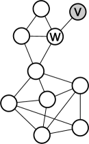
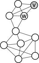
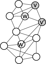
Figure 20: The Forest Fire burning process. Left: a new node $v$ joins the network and selects a seed node $w$. Middle: $v$ then attaches itself by recursively linking to $w$’s neighbors, $w$’s neighbor-neighbors, and so on, according to the “forest fire” burning mechanism described in the text. Right: a new node $v^{\prime}$ joins the network, selects seed $w^{\prime}$, and recursively adds links using the same “forest fire” burning mechanism. Notice that if $v^{\prime}$ causes a large “fire,” it links to a large number of existing nodes. In this way, as potential communities around node $w$ grow, the NCP plot is initially decreasing, but then larger communities around $w$ gradually blend-in with the rest of the network, which leads the NCP plot to increase.

Two properties of this model are particularly significant. First, although many nodes might form one or a small number of links, certain nodes can produce large conflagrations, burning many edges and thus forming a large number of out-links before the process ends. Such nodes will help generate a skewed out-degree distribution, and they will also serve as “bridges” that connect formerly disparate parts of the network. This will help make the NCP plot gradually increase. Second, there is a locality structure in that as each new node $v$ arrives over time, it is assigned a “center of gravity” in some part of the network, i.e., at the ambassador node $w$, and the manner in which new links are added depends sensitively on the local graph structure around node $w$. Not only does the probability of linking to other nodes decrease rapidly with distance to the current ambassador, but because of the recursive process regions with a higher density of links tend to attract new links.

Figure 20 illustrates this. Initially, there is a small community around node $w$. Then, node $v$ joins and using the Forest Fire mechanism locally attaches to nodes in the neighborhood of seed node $w$. The growth of the community around $w$ corresponds to downward part of the NCP plot. However, if a node $v^{\prime}$ then joins and causes a large fire, this has the effect of larger and larger communities around $w$ blending into and merging with the rest of the network.

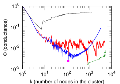
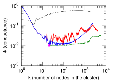
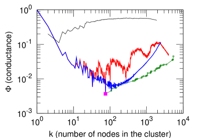
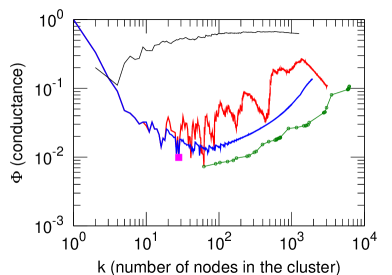
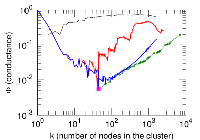
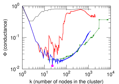
Figure 21: [Best viewed in color.] Community profile plots for the Forest Fire Model at various parameter settings. The backward burning probability is $p_{b}=0.3$, and we increase (left to right, top to bottom) the forward burning probability $p_{f}=\{0.26,0.31,0.33,0.35,0.37,0.40\}$. Note that the largest and smallest values for $p_{f}$ lead to less realistic community profile plots, as discussed in the text.

Not surprisingly, however, the Forest Fire Model is sensitive to the choice of the burning probabilities $p_{f}$ and $p_{b}$. We have experimented with a wide range of network sizes and values for these parameters, and in Figure 21, we show the community profile plots of several $10,000$ node Forest Fire networks generated with $p_{b}=0.3$ and several different values of $p_{f}$. The first thing to note is that since we are varying $p_{f}$ the six plots in Figure 21, we are viewing networks with very different densities. Next, notice that if, e.g., $p_{f}=0.33$ or $p_{f}=0.35$ then we observe a very natural behavior: the conductance nicely decreases, reaches the minimum somewhere between $10$ and $100$ nodes, and then slowly but not too smoothly increases. Not surprisingly, it is in this parameter region where the Forest Fire Model has been shown to exhibit realistic time evolving graph properties such as densification and shrinking diameters [112, 113].

Next, also notice that if $p_{f}$ is too low or too high, then we obtain qualitatively different results. For example, if $p_{f}=0.26$, then the community profile plot gradually decreases for nearly the entire plot. For this choice of parameters, the Forest Fire does not spread well since the forward burning probability is too small, the network is extremely sparse and is tree-like with just a few extra edges, and so we get large well separated “communities” that get better as they get larger. On the other hand, when burning probability is too high, e.g., $p_{f}=0.40$, then the NCP plot has a minimum and then rises extremely rapidly. For this choice of parameters, if a node which initially attached to a whisker successfully burns into the core, then it quickly establishes many successful connections to other nodes in the core. Thus, the network has relatively large whiskers that failed to establish such a connection and a very expander-like core, with no intermediate region, and the increase in the community profile plot is quite abrupt.

We have examined numerous other properties of the graphs generated by the Forest Fire Model and have found them to be broadly consistent with the social and information networks we have examined. One property, however, that is of particular interest is what the whiskers look like. Figure 22 shows an example of several whiskers generated by the Forest Fire Model if we choose $p_{b}=0.30$ and $p_{f}=0.37$. They are larger and more well-structured than the tree-like whiskers from the random graph model of Section 6.2. Also notice that they all look plausibly community-like with a core of the nodes densely linked among themselves and the bridge edge then connects the whisker to the rest of the network.

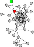
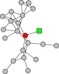
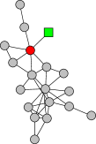
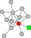
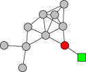
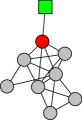
Figure 22: Examples of whiskers from a simulation of the Forest Fire Model with parameter settings $p_{f}=0.37$ and $p_{b}=0.3$. The green square node belongs to the network core, and by cutting the edge connecting it with red circular node we separate the community of circles from the rest of the network (depicted as a green square).

We conclude by noting that there has also been interest in developing hierarchical graph generation models, i.e., models in which a hierarchy is given and the linkage probability between pairs of nodes decreases as a function of their distance in the hierarchy [139, 138, 31, 6, 110, 48, 159, 111]. The motivation for this comes largely from the intuition that nodes in social networks and are joined in to small relatively tight groups that are then further join into larger groups, and so on. As Figures 17(c) and 17(d) make clear, however, such models do not immediately lead to community structure similar to what we have observed and which has been reproduced by the Forest Fire Model. On the other hand, although there are significant differences between hierarchical models and the Forest Fire Model, [112, 113] notes that there are similarities. In particular, in the Forest Fire Model a new node $v$ is assigned an ambassador $w$ as an entry point to the network. This is analogous to a child having a parent in the hierarchy which helps to determine how that node links to the remainder of the network. Similarly, many hierarchical models have a connection probability that decreases exponentially in the hierarchical tree distance. In the Forest Fire Model, the probability that a node $v$ will burn along a particular path to another node $u^{\prime}$ is exponentially small in the path length, although the analogy is not perfect since there may exist many possible paths.

7 Discussion

In this section, we discuss several aspects of our main results in a broader context. In particular, in Section 7.1, we compare to several data sets in which there is some notion of “ground truth” community and we also describe several broader non-technical implications of our results. Then, in Section 7.3, we describe recent work on community detection and identification. Finally, in Section 7.4, we discuss several technical and algorithmic issues and questions raised by our work.

7.1 Comparison with “ground truth” and sociological communities

In this subsection, we examine the relationship between network communities of the sort we have been discussing so far and some notion of “ground truth.” When considering a real network, one hopes that the output of a community finding algorithms will be “real” communities that exist in some meaningful sense in the real world. For example, in the Karate club network in Figure 5(a), the cut found by the algorithm corresponds in some sense to a true community, in that it splits the nodes almost precisely as they split into two newly formed karate clubs. In this section, we take a different approach: we take networks in which there are explicitly defined communities, and we examine how well these communities are separated from the rest of the network. In particular, we examine a minimum conductance profile of several network datasets, where we can associate with each node one or more community labels which are exogenously specified. Note that we are overloading the term “community” here, as in this context the term might mean one of two things: first, it can refer to groups of nodes with good conductance properties; and second, it can refer to groups of nodes that belong to the same self-defined or exogenously-specified group.

We consider the following five datasets:

• LiveJournal12 [20]: LiveJournal is an on-line blogging site where users can create friendship links to other users. In addition, users can create groups which other users can then join. In LiveJournal, there are $385,959$ such groups, and a node belongs to $3.5$ groups on the average. Thus, in addition to the information in the interaction graph, we have labels specifying those groups with which a user is associated, and thus we may view each such group as determining a “ground truth” community.

• CA-DBLP [20]: We considered a co-authorship network in which nodes are authors and there is an edge if authors co-authored at least one paper. Here, publication venues (e.g., journals and conferences) can play the role of “ground truth” communities. That is, an author is a member of a particular group or community if he or she published at a particular conference or in a particular journal. In our DBLP network, there are $2,547$ such groups, with a node belonging to $2.6$ on the average.

• AmazonAllProd [49]: This is a network of products that are commonly purchased together at amazon.com. (Intuitively one might expect that, e.g., gardening books are frequently purchased together, so the network structure might reflect a well-connected cluster of gardening books.) Here, each item belongs to one or more hierarchically organized categories (book, movie genres, product types, etc.), and products from the same category define a group which we will view as a “ground truth” community. Items can belong to $49,732$ different groups, and each item belongs to $14.3$ groups on the average.

• AtM-IMDB: This network is a bipartite actors-to-movies network composed from IMDB data, and an actor $A$ is connected to movie $B$ if $A$ appeared in $B$. For each movie we also know the language and the country where it was produced. Countries and languages may be taken as “ground truth” communities or groups, where every movie belongs to exactly one group and actors belongs to all groups to which movies that they appeared in belong. In our dataset, we have $393$ language groups and $181$ country groups.

• Email-Inside and Email-InOut [113]: This is an email communication network from a large European research organization conducting research in natural sciences: physics, chemistry, biology and computer science. Each of $986$ members of the organization belongs to exactly one of $45$ departments, and we use the department memberships to define “ground truth” communities.

Although none of these notions of “ground truth” is perfect, many community finding algorithms use precisely this form of anecdotal evaluation: a network is taken, network communities are found, and then the correspondence of network communities to “ground truth” communities is evaluated. Note, in contrast, we are evaluating how “ground truth” communities behave at different size scales with respect to our methodology, rather than examining how the groups we find relate to “ground truth” communities. Furthermore, note that the notions of “ground truth” are not all the same—we might expect that people publish papers across several different venues in a very different way than actors appear in movies from different countries. More detailed statistics for each of these networks may be found in Tables 1, 2 and 3.

To examine the quality of “ground truth” communities in the these network datasets, we take all groups and measure the conductance of the cut that separates that group from the rest of the network. Thus, we generated NCP plots in the following way. For every “ground truth” community, we measure the conductance of the cut separating it from the rest of the graph, from which we obtain a scatter plot of community size versus conductance. Then, we take the lower-envelope of this plot, i.e., for every integer $k$ we find the conductance value of the community of size $k$ that has the lowest conductance. Figure 23 shows the results for these network datasets; the figure also shows the NCP plot obtained from using the Local Spectral Algorithm on both the original network (plotted in red) and on the rewired network (plotted in black).

       

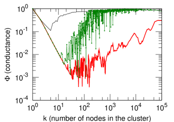
(a) LiveJournal12

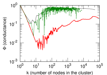
(b) CA-DBLP

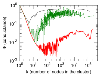
(c) AmazonAllProd

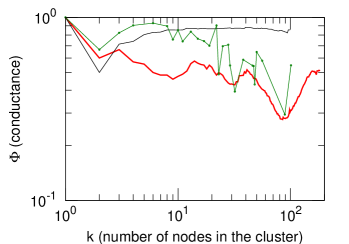
(d) Email-Inside

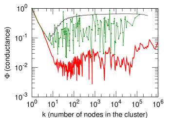
(e) AtM-IMDB Country

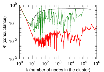
(f) AtM-IMDB Language

Figure 23: [Best viewed in color.] Network community profile plots for explicitly “ground truth” communities (green), compared with that for the original network (red) and a rewired version of the network (black): (a) LiveJournal12; (b) CA-DBLP; (c) AmazonAllProd; (d) Email-Inside; and (e-f) AtM-IMDB.

Several observations can be made:

• The conductance of “ground truth” communities follows that for the network communities up to until size $10$-$100$ nodes, i.e., larger communities get successively more community-like. As “ground truth” communities get larger, their conductance values tend to get worse and worse, in agreement with network communities discovered with graph partitioning approximation algorithms. Thus, the qualitative trend we observed in nearly every large sparse real-world network (of the best communities blending in with the rest of the network as they grow in size) is seen to hold for small “ground truth” communities.

• One might expect that the NCP plot for the “ground truth” communities (the green curves) will be somewhere between the NCP plot of the original network (red curves) and that for the rewired network (black curves), and this is seen to be the case in general. The NCP plot for network communities goes much deeper and rises more gradually than for “ground truth” communities. This is also consistent with our general observation that only small communities tend to be dense and well separated, and to separate large groups one has to cut disproportionately many edges.

• For the two social networks we studied (LiveJournal12 and CA-DBLP), larger “ground truth” communities have conductance scores that get quite “random”, i.e., they are as well separated as they would be in a randomly rewired network (green and black curves overlap). This is likely associated with the relatively weak and overlapping notion of “ground truth” we associated with those two network datasets. On the other hand, for AmazonAllProd and AtM-IMDB networks, the general trend still remains but large “ground truth” communities have conductance scores that lie well below the rewired network curve.

Our email network illustrates a somewhat different point. The NCP plot for Email-Inside should be compared with that for Email-InOut, which is displayed in Figure 7. The Email-Inside email network is rather small, and so it has a decreasing community profile plot, in agreement with the results for small social networks. Since communication is mainly focused between the members of the same department, both network and “ground truth” communities are well expressed. Next, compare the NCP plot of Email-Inside with that of Email-InOut (Figure 7). We see that the NCP plot of Email-Inside slopes downwards (as we consider only the communication inside the organization), but as soon as we consider the communication inside the organization and to the outside world (Email-InOut, or alternatively, see Email-Enron) then we see a completely different and more familiar picture—the NCP plot drops and then slowly increases. This suggests that the organizational structure, (e.g., departments) manifest themselves in the internal communication network, but as soon as we put the organization into the broader context (i.e., how it communicates to the rest of the world) then the internal department structure seems to disappear.

7.2 Connections and broader implications

In contrast to numerous studies of community structure, we find that there is a natural size scale to communities. Communities are relatively small, with sizes only up to about $100$ nodes. We also find that above size of about $100$, the “quality” of communities gets worse and worse and communities more and more “blend into” the network. Eventually, even the existence of communities (at least when viewed as sets with stronger internal than external connectivity) is rather questionable. We show that large social and information networks can be decomposed into a large number of small communities and a large dense and intermingled network “core”—we empirically establish that the “core” contains on average $60\%$ of the nodes and $80\%$ of all edges. But, as demonstrated by Figure 13, the “core” itself has a nontrivial structure—in particular, it has a core-whisker structure that is analogous to the original complete network.

The Dunbar number: Our observation on the limit of community size agrees with Dunbar [59] who predicted that roughly $150$ is the upper limit on the size of a well-functioning human community. Moreover, Allen [12] gives evidence that on-line communities have around $60$ members, and on-line discussion forums start to break down at about $80$ active contributors. Church congregations, military companies, divisions of corporations, all are close to the sum of $150$ [12]. We are thus led to ask: Why, above this size, is community quality inversely proportional to its size? And why are NCP plots of small and large networks so different?

Previous studies mainly focused on small networks (e.g., see [53]), which are simply not large enough for the clusters to gradually blend into one another as one looks at larger size scales. Our results do not disagree with literature at small sizes. But it seems that in order to make our observations one needs to look at large networks. It is only when Dunbar’s limit is passed that we find large communities blurring and eventually vanishing. A second reason is that previous work did not measure and examine the network community profile of cluster size vs. cluster quality.

Common bond vs. common identity communities: Dunbar’s explanation aligns well with the common bond vs. common identity theory of group attachment [141] from social psychology. Common identity theory makes predictions about people’s attachment to the group as a whole, while common bond theory predicts people’s attachment to individual group members. The distinction between the two refers to people’s different reasons for being in a group. Because they like the group as a whole we get identity-based attachment, or because they like individuals in the group we get bond-based attachment. Anecdotally, bond-based groups are based on social interaction with others, personal knowledge of them, and interpersonal attraction to them. On the other hand, identity-based groups are based on common identity of its members, e.g., liking to play a particular on-line game, contributing to Wikipedia, etc. It has been noted that bond communities tend to be smaller and more cohesive [19], as they are based on interpersonal ties, while identity communities are focused around common theme or interest. See [141] for a very good review of the topic.

Translating this to our context, the bond vs. identity communities mean that small, cohesive and well-separated communities are probably based on common bonds, while bigger groups may be based on common identity, and it is hard to expect such big communities to be well-separated or well-expressed in a network sense. This further means the transition between common bond (i.e., maintaining close personal ties) and common identity (i.e., sharing a common interest or theme) occurs at around one hundred nodes. It seems that at this size the cost of maintaining bond ties becomes too large and the group either dies or transitions into a common identity community. It would be very interesting as a future research topic to explore differences in community network structure as the community grows and transitions from common bond to common identity community.

Edge semantics: Another explanation could be that in small, carefully collected networks, the semantics of edges is very precise while in large networks we know much less about each particular edge, e.g., especially when online people have very different criteria for calling someone a friend. Traditionally social scientists through questionnaires “normalized” the links by making sure each link has the same semantics/strength.

Evidence in previous work: There has also been some evidence that hints towards the findings we make here. For example, Clauset et al. [49] analyzed community structure of a graph related to the AmazonAllProd, and they found that around $50\%$ of the nodes belonged to the largest “miscellaneous” community. This agrees with the typical size of the network core, and one could conclude that the largest community they found likely corresponds to the intermingled core of the network, and most of the rest of the communities are whisker-like.

In addition, recently there have been several works hinting that the network communities subject is more complex than it seems at the first sight. For example, it has been found that even random graphs can have good modularity scores [85]. Intuitively, random graphs have no community structure, but there can still exist sets of nodes with good community scores, at least as measured by modularity (due to random fluctuations about the mean). Moreover, very recently a study of robustness of community structure showed that the canonical example of presence of community structure in networks [160] may have no significant community structure [94].

More general thoughts: Our work also raises an important question of what is a natural community size and whether larger communities (in a network sense) even exist. It seems that when community size surpasses some threshold, the community becomes so diverse that it stops existing as a traditionally understood “network community.” Instead, it blends in with the network, and intuitions based on connectivity and cuts seem to fail to identify it. Approaches that consider both the network structure and node attribute data might help to detect communities in these cases.

Also, conductance seems like a very reasonable measure that satisfies intuition about community quality, but we have seen that if one only worries about conductance, then bags of whiskers and other internally disconnected sets have the best scores. This raises interesting questions about cluster compactness, regularization, and smoothness: what is a good definition of compactness, what is the best way to regularize these noisy networks, and how should this be connected to the notion of community separability?

A common assumption is that each node belongs to exactly one community. Our approach does not make such an assumption. Instead, for each given size, we independently find best set of nodes, and “communities” of different sizes often overlap. As long there is a boundary between communities (even if boundaries overlap), cut- and edge-density- based techniques (like modularity and conductance) may have the opportunity to find those communities. However, it is the absence of clear community boundaries that makes the NCP plot go upwards.

7.3 Relationship with community identification methods

A great deal of work has been devoted to finding communities in large networks, and much of this has been devoted to formalizing the intuition that a community is a set of nodes that has more and/or better intra-linkages between its members than inter-linkages with the remainder of the network. Very relevant to our work is that of Kannan, Vempala, and Vetta [93], who analyze spectral algorithms and describe a community concept in terms of a bicriterion depending on the conductance of the communities and the relative weight of inter-community edges. Flake, Tarjan, and Tsioutsiouliklis [69] introduce a similar bicriterion that is based on network flow ideas, and Flake et al. [67, 68] defined a community as a set of nodes that has more intra-edges than inter-edges. Similar edge-counting ideas were used by Radicchi et al. [136] to define and apply the notions of a strong community and a weak community.

Within the “complex networks” community, Girvan and Newman [80] proposed an algorithm that used “centrality” indices to find community boundaries. Following this, Newman and Girvan [132] introduced modularity as a posteriori measure of the strength of community structure. Modularity measures inter- (and not intra-) connectivity, but it does so with reference to a randomized null model. Modularity has been very influential in the recent community detection literature [128, 53], and one can use spectral techniques to approximate it [157, 131]. On the other hand, Guimerà, Sales-Pardo, and Amaral [85] and Fortunato and Barthélemy [73] showed that random graphs have high-modularity subsets and that there exists a size scale below which communities cannot be identified. In part as a response to this, some recent work has had a more statistical flavor [86, 140, 144, 94, 133]. In light of our results, this work seems promising, both due to potential “overfitting” issues arising from the extreme sparsity of the networks, and also due to the empirically-promising regularization properties exhibited by local spectral methods.

We have made extensive use of the Local Spectral Algorithm of Andersen, Chung, and Lang [13]. Similar results were originally proven by Spielman and Teng [150, 151], who analyzed local random walks on a graph; see Chung [35, 37, 36] for an exposition of the relationship between these methods. Andersen and Lang [14] showed that these techniques can find (in a scalable manner) medium-sized communities in very large social graphs in which there exist reasonably well-defined communities. In light of our results, such methods seem promising more generally. Other recent work that has focused on developing local and/or near-linear time heuristics for community detection include [49, 158, 47, 21, 137].

In addition to this work we have cited, there exists work which views communities from a very different perspective. For example, Kumar et al. [103] view communities as a dense bipartite subgraph of the Web; Gibson, Kleinberg, and Raghavan [79] view communities as consisting of a core of central authoritative pages linked together by hub pages; Hopcroft et al. [89, 90] are interested in the temporal evolution of communities that are robust when the input data to clustering algorithms that identify them are moderately perturbed; and Palla et al. [134] view communities as a chain of adjacent cliques and focus on the extent to which they are nested and overlap. The implications of our results for this body of work remain to be explored.

7.4 Relationship with other theoretical work

In this subsection, we describe the relationship between our work and recent work with similar flavor in graph partitioning, algorithms, and graph theory.

Recent work has focused on the expansion properties of power law graphs and the real-world networks they model. For example, Mihail, Papadimitriou, and Saberi [121], as well as Gkantsidis, Mihail, and Saberi [81], studied Internet routing at the level of Autonomous Systems (AS), and showed that the preferential attachment model and a random graph model with power law degree distributions each have good expansion properties if the minimum degree is greater than $2$ or $3$, respectively. This is consistent with the empirical results, but as we have seen the AS graphs are quite unusual, when compared with nearly every other social and information network we have studied. On the other hand, Estrada has made the observation that although certain communication, information, and biological networks have good expansion properties, social networks do not [60]. This is interpreted as evidence that such social networks have good small highly-cohesive groups, a property which is not attributed to the biological networks that were considered. From the perspective of our analysis, these results are interesting since it is likely that these small highly-cohesive groups correspond to sets near the global minimum of the network community profile plot. Reproducing deep cuts was also a motivation for the development of the geometric preferential attachment models of Flaxman, Frieze, and Vera [71, 72]. Note, however, that the deep cuts they obtain arise from the underlying geometry of the model and thus are nearly bisections.

Consider also recent results on the structural and spectral properties of very sparse random graphs. Recall that the $G_{np}$ random graph model [24] consists of those graphs on $n$ nodes, in which there is an edge between every pair vertices with a probability $p$, independently. Recall also that if $p\in(1/n,\log n/n)$, then a typical graph in $G_{np}$ has a giant component, i.e., connected subgraph consisting of a constant fraction of the nodes, but the graph is not fully connected [24]. (If $p<1/n$, the a typical graph is disconnected and there does not exist a giant component, while if $p>\log n/n$, then a typical graph is fully connected.) As noted, e.g., by Feige and Ofek [63], this latter regime is particularly difficult to analyze since with fairly high probability there exist vertices with degrees that are much larger than their expected degree. As reviewed in Section 6.2, however, this regime is not unlike that in a power law random graph in which the power law exponent $\beta\in(2,3)$ [38, 118, 42].

Chakrabarti et al. [30] defined the “min-cut” plot which has similarities with our NCP plot. They used a different approach in which a network was recursively bisected and then the quality of the obtained clusters was plotted against as a function of size; and the “min-cut” plots were only used as yet-another statistic to test when assessing how realistic are synthetically generated graphs. Note, however, that the “min-cut” plots have qualitatively similar behavior to our NCP plots, i.e., they initially decrease, reach a minimum, and then increase.

Of particular interest to us are recent results on the mixing time of random walks in this $p\in(1/n,\log n/n)$ regime of the $G_{np}$ (and the related $G_{nm}$) random graph model. Benjamini, Kozma, and Wormald [22] and Fountoulakis and Reed [75, 74] have established rapid mixing results by proving structural results about these very sparse graphs. In particular, they proved that these graphs may be viewed as a “core” expander subgraph, whose deletion leaves a large number of “decorations,” i.e., small components such that a bounded number are attached to any vertex in the core. The particular constructions in their proofs is complicated, but they have a similar flavor to the core-and-whiskers structure we have empirically observed. Similar results were observed by Fernholz and Ramachandran [64], whose analysis separately considered the $2$-core of these graphs and then the residual pieces. They show that a typical longest shortest path between two vertices $u$ and $v$ consists of a path of length $O(\log n)$ from $u$ to the $2$-core, then a path of length $O(\log n)$ across the $2$-core, and finally a path of length $O(\log n)$ from the $2$-core to $v$. Again, this is reminiscent of the core-and-whiskers properties we have observed. In all these cases, the structure is very different than traditional expanders [88], which we also empirically observe. Eigenvalues of power law graphs have also been studied by Mihail and Papadimitriou [120], Chung, Lu, Vu [44, 45, 46], and Flaxman, Frieze, and Fenner [70].

8 Conclusion

We investigated statistical properties of community-like sets of nodes in large real-world social and information networks. We discovered that community structure in these networks is very different than what we expected from the experience with small networks and from what commonly-used models would suggest.

In particular, we defined a network community profile plot (NCP plot), and we observed that good network communities exist only up to a size scale of $\approx 100$ nodes. This agrees well with the observations of Dunbar. For size scales above $\approx 100$ nodes, the NCP plot slopes upwards as the conductance score of the best possible set of nodes gets gradually worse and worse as those sets increase in size. Thus, if the world is modeled by a sparse “interaction graph” and if a density-based notion such as conductance is an appropriate measure of community quality, then the “best” possible “communities” in nearly every real-world network we examined gradually gets less and less community-like and instead gradually “blends in” with the rest of the network, as the purported communities steadily grow in size. Although this suggests that large networks have a core-periphery or jellyfish type of structure, where small “whiskers” connect themselves into a large dense intermingled network “core,” we also observed that the “core” itself has an analogous core-periphery structure.

None of the commonly-used network generation models, including preferential-attachment, copying, and hierarchical models, generates networks that even qualitatively reproduce this community structure property. We found, however, that a model in which edges are added recursively, via an iterative “forest fire” burning mechanism, produces remarkably good results. Our work opens several new questions about the structure of large social and information networks in general, and it has implications for the use of graph partitioning algorithms on real-world networks and for detecting communities in them.

References

- [1] University of Oregon Route Views Project. Online data and reports. http://www.routeviews.org, 1997.
- [2] TREC Web Corpus: WT10g. http://ir.dcs.gla.ac.uk/test_collections/wt10g.html, 2000.
- [3] Google Programming Contest. http://www.google.com/programming-contest/, 2002.
- [4] Netflix prize. http://www.netflixprize.com/, 2006.
- [5] Network data. http://www-personal.umich.edu/~mejn/netdata/, July 16, 2007.
- [6] J. Abello. Hierarchical graph maps. Computers and Graphics, 28(3):345–359, 2004.
- [7] W. Aiello, F.R.K. Chung, and L. Lu. A random graph model for massive graphs. In STOC ’00: Proceedings of the 32nd annual ACM Symposium on Theory of Computing, pages 171–180, 2000.
- [8] W. Aiello, F.R.K. Chung, and L. Lu. A random graph model for power law graphs. Experimental Mathematics, 10:53–66, 2001.
- [9] R. Z. Albert and A-L. Barabási. Emergence of scaling in random networks. Science, 286(5439):509–512, 1999.
- [10] R. Z. Albert and A-L. Barabási. Statistical mechanics of complex networks. Reviews of Modern Physics, 74:47–97, 2002.
- [11] R. Z. Albert, H. Jeong, and A-L. Barabási. The diameter of the world wide web. Nature, 401:130–131, 1999.
- [12] Christopher Allen. Life with alacrity: The Dunbar number as a limit to group sizes, 2004.
- [13] R. Andersen, F.R.K. Chung, and K. Lang. Local graph partitioning using PageRank vectors. In FOCS ’06: Proceedings of the 47th Annual IEEE Symposium on Foundations of Computer Science, pages 475–486, 2006.
- [14] R. Andersen and K. Lang. Communities from seed sets. In WWW ’06: Proceedings of the 15th International Conference on World Wide Web, pages 223–232, 2006.
- [15] S. Arora, E. Hazan, and S. Kale. approximation to sparsest cut in time. In FOCS ’04: Proceedings of the 45th Annual Symposium on Foundations of Computer Science, pages 238–247, 2004.
- [16] S. Arora and S. Kale. A combinatorial, primal-dual approach to semidefinite programs. In STOC ’07: Proceedings of the 39th annual ACM Symposium on Theory of Computing, pages 227–236, 2007.
- [17] S. Arora, S. Rao, and U. Vazirani. Expander flows, geometric embeddings and graph partitioning. In STOC ’04: Proceedings of the 36th annual ACM Symposium on Theory of Computing, pages 222–231, 2004.
- [18] M. Babenko, J. Derryberry, A. Goldberg, R. Tarjan, and Y. Zhou. Experimental evaluation of parametric max-flow algorithms. In WEA ’07: Proceedings of the 6th Workshop on Experimental Algorithms, pages 256–269, 2007.
- [19] K.W. Back. Influence through social communication. Journal of Abnormal and Social Psychology, 46:9–23, 1951.
- [20] L. Backstrom, D. Huttenlocher, J. Kleinberg, and X. Lan. Group formation in large social networks: membership, growth, and evolution. In KDD ’06: Proceedings of the 12th ACM SIGKDD International Conference on Knowledge Discovery and Data Mining, pages 44–54, 2006.
- [21] J.P. Bagrow and E.M. Bollt. Local method for detecting communities. Physical Review E, 72:046108, 2005.
- [22] I. Benjamini, G. Kozma, and N. Wormald. The mixing time of the giant component of a random graph. arXiv:math/0610459, October 2006.
- [23] S. Boccaletti, V. Latora, Y. Moreno, M. Chavez, and D.U. Hwang. Complex networks: Structure and dynamics. Physics Reports, 424(4-5):175–308, 2006.
- [24] B. Bollobás. Random Graphs. Academic Press, London, 1985.
- [25] B. Bollobás and O. M. Riordan. Mathematical results on scale-free random graphs. In S. Bornholdt and H.G. Schuster, editors, Handbook of Graphs and Networks, pages 1–34. Wiley, 2004.
- [26] U. Brandes, M. Gaertler, and D. Wagner. Engineering graph clustering: Models and experimental evaluation. Journal of Experimental Algorithmics, 12(1), 2007.
- [27] A. Broder, R. Kumar, F. Maghoul, P. Raghavan, S. Rajagopalan, R. Stata, A. Tomkins, and J. Wiener. Graph structure in the Web. In WWW ’00: Proceedings of the 9th International Conference on World Wide Web, pages 309–320, 2000.
- [28] S. Burer and R.D.C. Monteiro. A nonlinear programming algorithm for solving semidefinite programs via low-rank factorization. Mathematical Programming (series B), 95(2):329–357, 2003.
- [29] D. Chakrabarti and C. Faloutsos. Graph mining: Laws, generators, and algorithms. ACM Computing Surveys, 38(1):2, 2006.
- [30] D. Chakrabarti, C. Faloutsos, and Y. Zhan. Visualization of large networks with min-cut plots, A-plots and R-MAT. International Journal of Human-Computer Studies, 65(5):434–445, 2007.
- [31] D. Chakrabarti, Y. Zhan, and C. Faloutsos. R-MAT: A recursive model for graph mining. In SDM ’04: Proceedings of the 4th SIAM International Conference on Data Mining, 2004.
- [32] J. Cheeger. A lower bound for the smallest eigenvalue of the laplacian. In Problems in Analysis, Papers dedicated to Salomon Bochner, pages 195–199. Princeton University Press, 1969.
- [33] B.V. Cherkassky and A.V. Goldberg. On implementing push-relabel method for the maximum flow problem. In IPCO ’95: Proceedings of the 4th International IPCO Conference on Integer Programming and Combinatorial Optimization, pages 157–171, 1995.
- [34] F.R.K. Chung. Spectral graph theory, volume 92 of CBMS Regional Conference Series in Mathematics. American Mathematical Society, 1997.
- [35] F.R.K Chung. Four proofs of cheeger inequality and graph partition algorithms. In Proceedings of ICCM, 2007.
- [36] F.R.K. Chung. The heat kernel as the pagerank of a graph. Proceedings of the National Academy of Sciences of the United States of America, 104(50):19735–19740, 2007.
- [37] F.R.K. Chung. Random walks and local cuts in graphs. Linear Algebra and its Applications, 423:22–32, 2007.
- [38] F.R.K. Chung and L. Lu. The diameter of sparse random graphs. Advances in Applied Mathematics, 26(4):257–279, 2001.
- [39] F.R.K. Chung and L. Lu. The average distances in random graphs with given expected degrees. Proceedings of the National Academy of Sciences of the United States of America, 99(25):15879–15882, 2002.
- [40] F.R.K. Chung and L. Lu. Connected components in random graphs with given expected degree sequences. Annals of Combinatorics, 6(2):125–145, 2002.
- [41] F.R.K. Chung and L. Lu. The average distances in a random graph with given expected degrees. Internet Mathematics, 1:91–113, 2003.
- [42] F.R.K. Chung and L. Lu. Complex Graphs and Networks, volume 107 of CBMS Regional Conference Series in Mathematics. American Mathematical Society, 2006.
- [43] F.R.K. Chung and L. Lu. The volume of the giant component of a random graph with given expected degrees. SIAM Journal on Discrete Mathematics, 20:395–411, 2006.
- [44] F.R.K. Chung, L. Lu, and Van Vu. Eigenvalues of random power law graphs. Annals of Combinatorics, 7:21–33, 2003.
- [45] F.R.K. Chung, L. Lu, and Van Vu. The spectra of random graphs with given expected degrees. Proceedings of the National Academy of Sciences of the United States of America, 100(11):6313–6318, 2003.
- [46] F.R.K. Chung, L. Lu, and Van Vu. The spectra of random graphs with given expected degrees. Internet Mathematics, 1:257–275, 2004.
- [47] A. Clauset. Finding local community structure in networks. Physical Review E, 72:026132, 2005.
- [48] A. Clauset, C. Moore, and M.E.J. Newman. Structural inference of hierarchies in networks. arXiv:physics/0610051, October 2006.
- [49] A. Clauset, M.E.J. Newman, and C. Moore. Finding community structure in very large networks. arXiv:cond-mat/0408187, August 2004.
- [50] A. Clauset, C.R. Shalizi, and M.E.J. Newman. Power-law distributions in empirical data. arXiv:0706.1062, June 2007.
- [51] V. Colizza, A. Flammini, M.A. Serrano, and A. Vespignani. Characterization and modeling of protein protein interaction networks. Physica A Statistical Mechanics and its Applications, 352:1–27, 2005.
- [52] L. da F. Costa, F.A. Rodrigues, G. Travieso, and P.R. Villas Boas. Characterization of complex networks: A survey of measurements. Advances in Physics, 56(1):167–242, 2007.
- [53] L. Danon, J. Duch, A. Diaz-Guilera, and A. Arenas. Comparing community structure identification. Journal of Statistical Mechanics: Theory and Experiment, 29(09):P09008, 2005.
- [54] I.S. Dhillon, Y. Guan, and B. Kulis. Weighted graph cuts without eigenvectors: A multilevel approach. IEEE Transactions on Pattern Analysis and Machine Intelligence, 29(11):1944–1957, 2007.
- [55] W.E. Donath and A.J. Hoffman. Algorithms for partitioning graphs and computer logic based on eigenvectors of connection matrices. IBM Technical Disclosure Bulletin, 15(3):938–944, 1972.
- [56] S.N. Dorogovtsev and J.F.F. Mendes. Evolution of networks. Advances in Physics, 51:1079–1187, 2002.
- [57] J. Doyle and J.M. Carlson. Power laws, highly optimized tolerance, and generalized source coding. Physical Review Letters, 84(24):5656–5659, 2000.
- [58] J. Doyle and J.M. Carlson. Complexity and robustness. Proceedings of the National Academy of Sciences of the United States of America, 99:2538–2545, 2002.
- [59] Robin Dunbar. Grooming, Gossip, and the Evolution of Language. Harvard Univ Press, October 1998.
- [60] E. Estrada. Spectral scaling and good expansion properties in complex networks. Europhysics Letters, 73:649–655, 2006.
- [61] A. Fabrikant, E. Koutsoupias, and C.H. Papadimitriou. Heuristically optimized trade-offs: A new paradigm for power laws in the Internet. In ICALP ’02: Proceedings of the 29th International Colloquium on Automata, Languages and Programming, pages 110–122, 2002.
- [62] M. Faloutsos, P. Faloutsos, and C. Faloutsos. On power-law relationships of the internet topology. In SIGCOMM ’99: Proceedings of the Conference on Applications, technologies, architectures, and protocols for computer communication, pages 251–262, 1999.
- [63] U. Feige and E. Ofek. Spectral techniques applied to sparse random graphs. Random Structures and Algorithms, 27:251–275, 2005.
- [64] D. Fernholz and V. Ramachandran. The diameter of sparse random graphs. Random Structures and Algorithms, 31:482–516, 2007.
- [65] C.M. Fiduccia and R.M. Mattheyses. A linear-time heuristic for improving network partitions. In DAC ’82: Proceedings of the 19th ACM/IEEE Conference on Design Automation, pages 175–181, 1982.
- [66] M. Fiedler. Algebraic connectivity of graphs. Czechoslovak Mathematical Journal, 23(98):298–305, 1973.
- [67] G.W. Flake, S. Lawrence, and C.L. Giles. Efficient identification of web communities. In KDD ’00: Proceedings of the 6th ACM SIGKDD International Conference on Knowledge Discovery and Data Mining, pages 150–160, 2000.
- [68] G.W. Flake, S. Lawrence, C.L. Giles, and F.M. Coetzee. Self-organization and identification of web communities. Computer, 35(3):66–71, 2002.
- [69] G.W. Flake, R.E. Tarjan, and K.Tsioutsiouliklis. Graph clustering and minimum cut trees. Internet Mathematics, 1(4):385–408, 2003.
- [70] A. Flaxman, A. Frieze, and T. Fenner. High degree vertices and eigenvalues in the preferential attachment graph. Internet Mathematics, 2(1):1–19, 2005.
- [71] A.D. Flaxman, A.M. Frieze, and J. Vera. A geometric preferential attachment model of networks. In WAW ’04: Proceedings of the 3rd Workshop On Algorithms And Models For The Web-Graph, pages 44–55, 2004.
- [72] A.D. Flaxman, A.M. Frieze, and J. Vera. A geometric preferential attachment model of networks II. In WAW ’07: Proceedings of the 5th Workshop On Algorithms And Models For The Web-Graph, pages 41–55, 2007.
- [73] S. Fortunato and M. Barthélemy. Resolution limit in community detection. Proceedings of the National Academy of Sciences of the United States of America, 104(1):36–41, 2007.
- [74] N. Fountoulakis and B. Reed. The evolution of the mixing rate. arXiv:math/0701474, January 2007.
- [75] N. Fountoulakis and B.A. Reed. Faster mixing and small bottlenecks. Probability Theory and Related Fields, 137(3–4):475–486, 2007.
- [76] M. Gaertler. Clustering. In U. Brandes and T. Erlebach, editors, Network Analysis: Methodological Foundations, pages 178–215. Springer, 2005.
- [77] G. Gallo, M.D. Grigoriadis, and R.E. Tarjan. A fast parametric maximum flow algorithm and applications. SIAM Journal on Computing, 18(1):30–55, 1989.
- [78] J. Gehrke, P. Ginsparg, and J. Kleinberg. Overview of the 2003 KDD Cup. SIGKDD Explorations, 5(2):149–151, 2003.
- [79] D. Gibson, J. Kleinberg, and P. Raghavan. Inferring web communities from link topology. In HT ’98: Proceedings of the 9th ACM Conference on Hypertext and Hypermedia, pages 225–234, 1998.
- [80] M. Girvan and M.E.J. Newman. Community structure in social and biological networks. Proceedings of the National Academy of Sciences of the United States of America, 99(12):7821–7826, 2002.
- [81] C. Gkantsidis, M. Mihail, and A. Saberi. Conductance and congestion in power law graphs. In Proceedings of the 2003 ACM SIGMETRICS International Conference on Measurement and modeling of computer systems, pages 148–159, 2003.
- [82] A.V. Goldberg and S. Rao. Beyond the flow decomposition barrier. Journal of the ACM, 45:783–797, 1998.
- [83] A.V. Goldberg and R.E. Tarjan. A new approach to the maximum-flow problem. Journal of the ACM, 35:921–940, 1988.
- [84] S. Guattery and G.L. Miller. On the quality of spectral separators. SIAM Journal on Matrix Analysis and Applications, 19:701–719, 1998.
- [85] R. Guimerà, M. Sales-Pardo, and L.A.N. Amaral. Modularity from fluctuations in random graphs and complex networks. Physical Review E, 70:025101, 2004.
- [86] M.B. Hastings. Community detection as an inference problem. Physical Review E, 74:035102, 2006.
- [87] B. Hendrickson and R. Leland. A multilevel algorithm for partitioning graphs. In Supercomputing ’95: Proceedings of the 1995 ACM/IEEE Conference on Supercomputing (CDROM), 1995.
- [88] S. Hoory, N. Linial, and A. Wigderson. Expander graphs and their applications. Bulletin of the American Mathematical Society, 43:439–561, 2006.
- [89] J. Hopcroft, O. Khan, B. Kulis, and B. Selman. Natural communities in large linked networks. In KDD ’03: Proceedings of the 9th ACM SIGKDD International Conference on Knowledge Discovery and Data Mining, pages 541–546, 2003.
- [90] J. Hopcroft, O. Khan, B. Kulis, and B. Selman. Tracking evolving communities in large linked networks. Proceedings of the National Academy of Sciences of the United States of America, 101:5249–5253, 2004.
- [91] A.K. Jain, M.N. Murty, and P.J. Flynn. Data clustering: a review. ACM Computing Surveys, 31:264–323, 1999.
- [92] H. Jeong, S.P. Mason, A-L. Barabási, and Z.N. Oltvai. Lethality and centrality in protein networks. Nature, 411:41–42, 2001.
- [93] R. Kannan, S. Vempala, and A. Vetta. On clusterings: Good, bad and spectral. Journal of the ACM, 51(3):497–515, 2004.
- [94] B. Karrer, E. Levina, and M.E.J. Newman. Robustness of community structure in networks. arXiv:0709.2108, September 2007.
- [95] G. Karypis and V. Kumar. A fast and high quality multilevel scheme for partitioning irregular graphs. SIAM Journal on Scientific Computing, 20:359–392, 1998.
- [96] G. Karypis and V. Kumar. Multilevel k-way partitioning scheme for irregular graphs. Journal of Parallel and Distributed Computing, 48:96–129, 1998.
- [97] B. Kernighan and S. Lin. An effective heuristic procedure for partitioning graphs. The Bell System Technical Journal, pages 291–308, 1970.
- [98] A. Khalil and Y. Liu. Experiments with PageRank computation. Technical Report 603, Indiana University Department of Computer Science, December 2004.
- [99] R. Khandekar, S. Rao, and U. Vazirani. Graph partitioning using single commodity flows. In STOC ’06: Proceedings of the 38th annual ACM Symposium on Theory of Computing, pages 385–390, 2006.
- [100] B. Klimt and Y. Yang. Introducing the enron corpus. In CEAS ’04: Proceedings of the 1st Conference on Email and Anti-Spam, 2004.
- [101] R. Kumar, J. Novak, and A. Tomkins. Structure and evolution of online social networks. In KDD ’06: Proceedings of the 12th ACM SIGKDD International Conference on Knowledge Discovery and Data Mining, pages 611–617, 2006.
- [102] R. Kumar, P. Raghavan, S. Rajagopalan, D. Sivakumar, A. Tomkins, and E. Upfal. Stochastic models for the web graph. In FOCS ’00: Proceedings of the 41st Annual Symposium on Foundations of Computer Science, pages 57–65, 2000.
- [103] R. Kumar, P. Raghavan, S. Rajagopalan, and A. Tomkins. Trawling the web for emerging cyber-communities. Computer Networks, 31(11):1481–1493, 1999.
- [104] K. Lang. Finding good nearly balanced cuts in power law graphs. Technical Report YRL-2004-036, Yahoo! Research Labs, Pasadena, CA, November 2004.
- [105] K. Lang and S. Rao. Finding near-optimal cuts: an empirical evaluation. In SODA ’93: Proceedings of the 4th annual ACM-SIAM Symposium on Discrete algorithms, pages 212–221, 1993.
- [106] K. Lang and S. Rao. A flow-based method for improving the expansion or conductance of graph cuts. In IPCO ’04: Proceedings of the 10th International IPCO Conference on Integer Programming and Combinatorial Optimization, pages 325–337, 2004.
- [107] T. Leighton and S. Rao. An approximate max-flow min-cut theorem for uniform multicommodity flow problems with applications to approximation algorithms. In FOCS ’88: Proceedings of the 28th Annual Symposium on Foundations of Computer Science, pages 422–431, 1988.
- [108] T. Leighton and S. Rao. Multicommodity max-flow min-cut theorems and their use in designing approximation algorithms. Journal of the ACM, 46(6):787–832, 1999.
- [109] J. Leskovec, L.A. Adamic, and B.A. Huberman. The dynamics of viral marketing. ACM Transactions on the Web, 1(1), 2007.
- [110] J. Leskovec, D. Chakrabarti, J. Kleinberg, and C. Faloutsos. Realistic, mathematically tractable graph generation and evolution, using kronecker multiplication. In ECML/PKDD ’05: Proceedings of the European International Conference on Principles and Practice of Knowledge Discovery in Databases, pages 133–145, 2005.
- [111] J. Leskovec and C. Faloutsos. Scalable modeling of real graphs using kronecker multiplication. In ICML ’07: Proceedings of the 24th International Conference on Machine Learning, pages 497–504, 2007.
- [112] J. Leskovec, J. Kleinberg, and C. Faloutsos. Graphs over time: densification laws, shrinking diameters and possible explanations. In KDD ’05: Proceeding of the 11th ACM SIGKDD International Conference on Knowledge Discovery in Data Mining, pages 177–187, 2005.
- [113] J. Leskovec, J. Kleinberg, and C. Faloutsos. Graph evolution: Densification and shrinking diameters. ACM Transactions on Knowledge Discovery from Data, 1(1), 2007.
- [114] J. Leskovec, K.J. Lang, A. Dasgupta, and M.W. Mahoney. Statistical properties of community structure in large social and information networks. Manuscript. March 7, 2008.
- [115] J. Leskovec, K.J. Lang, A. Dasgupta, and M.W. Mahoney. Statistical properties of community structure in large social and information networks. In WWW ’08: Proceedings of the 17th International Conference on World Wide Web, pages 695–704, 2008.
- [116] J. Leskovec, M. McGlohon, C. Faloutsos, N.S. Glance, and M. Hurst. Patterns of cascading behavior in large blog graphs. In SDM ’07: Proceedings of the 7th SIAM Conference on Data Mining, 2007.
- [117] L. Li, J.C. Doyle, and W. Willinger. Towards a theory of scale-free graphs: Definition, properties, and implications. Internet Mathematics, 2(4):431–523, 2006.
- [118] L. Lu. The diameter of random massive graphs. In SODA ’01: Proceedings of the 12th annual ACM-SIAM Symposium on Discrete algorithms, pages 912–921, 2001.
- [119] D. Lusseau, K. Schneider, O.J. Boisseau, P. Haase, E. Slooten, and S.M. Dawson. The bottlenose dolphin community of doubtful sound features a large proportion of long-lasting associations. Behavioral Ecology and Sociobiology, 54:396–405, 2003.
- [120] M. Mihail and C.H. Papadimitriou. On the eigenvalue power law. In RANDOM ’02: Proceedings of the 6th International Workshop on Randomization and Approximation Techniques, pages 254–262, 2002.
- [121] M. Mihail, C.H. Papadimitriou, and A. Saberi. On certain connectivity properties of the internet topology. Journal of Computer and System Sciences, 72(2):239–251, 2006.
- [122] R. Milo, N. Kashtan, S. Itzkovitz, M.E.J. Newman, and U. Alon. On the uniform generation of random graphs with prescribed degree sequences. arXiv:cond-mat/0312028v2, May 2004.
- [123] B. Mohar. The Laplacian spectrum of graphs. In Y. Alavi, G. Chartrand, O.R. Oellermann, and A.J. Schwenk, editors, Graph Theory, Combinatorics, and Applications, Vol. 2, pages 871–898. Wiley, 1991.
- [124] M. Molloy and B. Reed. A critical point for random graphs with a given degree sequence. Random Structures and Algorithms, 6:161–180, 1995.
- [125] M. Molloy and B. Reed. The size of the giant component of a random graph with a given degree sequence. Combinatorics, Probability and Computing, 7:295–305, 1998.
- [126] A.L. Montgomery and C. Faloutsos. Identifying web browsing trends and patterns. Computer, 34(7):94–95, 2001.
- [127] M.E.J. Newman. The structure and function of complex networks. SIAM Review, 45:167–256, 2003.
- [128] M.E.J. Newman. Detecting community structure in networks. The European Physical Journal B, 38:321–330, 2004.
- [129] M.E.J. Newman. Power laws, Pareto distributions and Zipf’s law. Contemporary Physics, 46:323–351, 2005.
- [130] M.E.J. Newman. Finding community structure in networks using the eigenvectors of matrices. Physical Review E, 74:036104, 2006.
- [131] M.E.J. Newman. Modularity and community structure in networks. Proceedings of the National Academy of Sciences of the United States of America, 103(23):8577–8582, 2006.
- [132] M.E.J. Newman and M. Girvan. Finding and evaluating community structure in networks. Physical Review E, 69:026113, 2004.
- [133] M.E.J. Newman and E.A. Leicht. Mixture models and exploratory analysis in networks. Proceedings of the National Academy of Sciences of the United States of America, 104(23):9564–9569, 2007.
- [134] G. Palla, I. Derényi, I. Farkas, and T. Vicsek. Uncovering the overlapping community structure of complex networks in nature and society. Nature, 435(7043):814–818, 2005.
- [135] Y. Qi, J.K. Seetharaman, and Z.B. Joseph. Random forest similarity for protein-protein interaction prediction from multiple sources. In Pacific Symposium on Biocomputing, 2005.
- [136] F. Radicchi, C. Castellano, F. Cecconi, V. Loreto, and D. Parisi. Defining and identifying communities in networks. Proceedings of the National Academy of Sciences of the United States of America, 101(9):2658–2663, 2004.
- [137] U. Nandini Raghavan, R.Z. Albert, and S. Kumara. Near linear time algorithm to detect community structures in large-scale networks. Physical Review E, 76:036106, 2007.
- [138] E. Ravasz and A.-L. Barabási. Hierarchical organization in complex networks. Physical Review E, 67:026112, 2003.
- [139] E. Ravasz, A.L. Somera, D.A. Mongru, Z.N. Oltvai, and A.-L. Barabási. Hierarchical organization of modularity in metabolic networks. Science, 297(5586):1551–1555, 2002.
- [140] J. Reichardt and S. Bornholdt. Partitioning and modularity of graphs with arbitrary degree distribution. Physical Review E, 76:015102, 2007.
- [141] Y. Ren, R. Kraut, and S. Kiesler. Applying common identity and bond theory to design of online communities. Organization Studies, 28(3):377–408, 2007.
- [142] M. Richardson, R. Agrawal, and P. Domingos. Trust management for the semantic web. In ISWC ’03: Proceedings of the 2nd International Semantic Web Conference, pages 351–368, 2003.
- [143] M. Ripeanu, I. Foster, and A. Iamnitchi. Mapping the gnutella network: Properties of large-scale peer-to-peer systems and implications for system design. IEEE Internet Computing, 6(1):50–57, 2002.
- [144] M. Rosvall and C.T. Bergstrom. An information-theoretic framework for resolving community structure in complex networks. Proceedings of the National Academy of Sciences of the United States of America, 104(18):7327–7331, 2007.
- [145] S.F. Sampson. A novitiate in a period of change: An experimental and case study of social relationships. Technical report, Cornell University Deptartment of Sociology PhD thesis, 1968.
- [146] S.E. Schaeffer. Graph clustering. Computer Science Review, 1(1):27–64, 2007.
- [147] J. Shi and J. Malik. Normalized cuts and image segmentation. IEEE Transcations of Pattern Analysis and Machine Intelligence, 22(8):888–905, 2000.
- [148] G. Siganos, S.L. Tauro, and M. Faloutsos. Jellyfish: A conceptual model for the as internet topology. Journal of Communications and Networks, 8:339–350, 2006.
- [149] D.A. Spielman and S.-H. Teng. Spectral partitioning works: Planar graphs and finite element meshes. In FOCS ’96: Proceedings of the 37th Annual IEEE Symposium on Foundations of Computer Science, pages 96–107, 1996.
- [150] D.A. Spielman and S.-H. Teng. Nearly-linear time algorithms for graph partitioning, graph sparsification, and solving linear systems. In STOC ’04: Proceedings of the 36th annual ACM Symposium on Theory of Computing, pages 81–90, 2004.
- [151] D.A. Spielman and S.-H. Teng. Nearly-linear time algorithms for graph partitioning, graph sparsification, and solving linear systems. arXiv:cs/0310051v9, March 2004.
- [152] S.L. Tauro, C. Palmer, G. Siganos, and M. Faloutsos. A simple conceptual model for the internet topology. In GLOBECOM ’01: Global Telecommunications Conference, pages 1667–1671, 2001.
- [153] J.B. Tenenbaum, V. de Silva, and J.C. Langford. A global geometric framework for nonlinear dimensionality reduction. Science, 290(5500):2319–2323, 2000.
- [154] U. von Luxburg. A tutorial on spectral clustering. Technical Report 149, Max Plank Institute for Biological Cybernetics, August 2006.
- [155] S. Wasserman and K. Faust. Social Network Analysis. Cambridge University Press, Cambridge, 1994.
- [156] D.J. Watts and S.H. Strogatz. Collective dynamics of small-world networks. Nature, 393:440–442, 1998.
- [157] S. White and P. Smyth. A spectral clustering approach to finding communities in graphs. In SDM ’05: Proceedings of the 5th SIAM International Conference on Data Mining, pages 76–84, 2005.
- [158] F. Wu and B.A. Huberman. Finding communities in linear time: a physics approach. The European Physical Journal B, 38(2):331–338, 2004.
- [159] Q. Xuan, Y. Li, and T.-J. Wu. Growth model for complex networks with hierarchical and modular structures. Physical Review E, 73:036105, 2006.
- [160] W.W. Zachary. An information flow model for conflict and fission in small groups. Journal of Anthropological Research, 33:452–473, 1977.
- [161] C.T. Zahn. Graph-theoretical methods for detecting and describing gestalt clusters. IEEE Transactions on Computers, C-20(1):68–86, 1971.
- [162] Y. Zhao and G. Karypis. Empirical and theoretical comparisons of selected criterion functions for document clustering. Machine Learning, 55:311–331, 2004.