Quantum fluctuations in trapped time-dependent Bose-Einstein condensates

Abstract

Quantum fluctuations in time-dependent, harmonically-trapped Bose-Einstein condensates are studied within Bogoliubov theory. An eigenmode expansion of the linear field operators permits the diagonalization of the Bogoliubov-de Gennes equation for a stationary condensate. When trap frequency or interaction strength are varied, the inhomogeneity of the background gives rise to off-diagonal coupling terms between different modes. This coupling is negligible for low energies, i.e., in the hydrodynamic regime, and an effective space-time metric can be introduced. The influence of the inter-mode coupling will be demonstrated in an example, where I calculate the quasi-particle number for a quasi-one-dimensional Bose-Einstein condensate subject to an exponential sweep of interaction strength and trap frequency.

I Introduction

Ultracold atomic gases offer various opportunities for the study of interacting many-body quantum systems in a well-controlled environment BEC ; Manybody . For instance, the Bose-Hubbard model – a simplified description for bosons in a periodic potential – can be studied with Bose-Einstein condensates confined in optical lattices Mott ; BHM . Quantum gases have also gained much attention lately regarding the emergence of an effective space-time Unruh ; Garay ; Review ; Piyush ; Silke ; Barcelo ; PeterF ; Uwe ; Uwe2 ; ich_njp ; Kurita ; WuesterBlackhole ; Matt ; Volovik ; artificialblackholes : their low-energy phase fluctuations obey the same covariant field equations as a scalar quantum field in a certain curved space-time. Hence, the study of phonons in this laboratory system might shed some light on aspects of cosmic quantum effects, e.g., Hawking radiation Hawking ; Garay ; WuesterBlackhole ; artificialblackholes ; Unruh or the freezing and amplification of quantum fluctuations in expanding spacetimes LL ; PeterF ; Uwe ; ich_njp ; Silke ; Piyush ; Barcelo ; BirrellDavis . Although the fluctuations in Bose-Einstein condensates are usually small, it has recently become possible in experiments to go beyond the classical order parameter and resolve signatures of the fluctuations noise-correlations ; interference ; Bragg ; ultracoldHBT ; numberfluct .

Theoretically, the fluctuations in a Bose-Einstein condensate are usually treated as small perturbations of the mean field. The solution of the coupled field equations is rather demanding and often requires further approximations, especially for time-dependent condensates. The Hartree-Fock-Bogoliubov method, see, e.g., Griffin , permits in principle the self-consistent propagation of the mean field and the quantum correlations for arbitrary time-dependences of the trap potential or interaction strength. But the scaling of the numerics with system size often limits the actual calculations to a low number of dimensions, certain symmetries, or a short time interval. Thermal condensates might be studied using the projected Gross-Pitaevskii equation projectedGP , where the low-energy part of the fluctuations is expanded into an arbitrary basis and, in view of the large thermal occupation, treated classically; higher excitations as well as the vacuum effect are omitted. On the other hand, studies in the context of expanding spacetimes, e.g., Silke ; Piyush ; ich_njp ; Uwe ; Barcelo ; Review ; Uwe2 , indeed focus on the quantum fluctuations but often assume a homogeneous background or start with the hydrodynamic action, which is only valid on scales longer than the healing length.

In this article, I will discuss the evolution of the quantum fluctuations in trapped time-dependent Bose-Einstein condensates. The linear field operators will be expanded into their eigenmodes thus permitting the diagonalization of the (initial) evolution equations. Although basis expansions of the field operator are frequently used (e.g., in projectedGP ; WuesterBosenova ), these references usually consider the harmonic oscillator eigenfunctions, a large number of which must be used in order to describe the excitations properly. By adopting the eigenmodes, a much smaller part of the basis needs to be considered and many more situations will become numerically feasible. (Note, however, that in order to obtain the fluctuation eigenmodes, a relatively large number of oscillator functions must be employed – but they need not be propagated.)

This Article is organized as follows. Section II reviews the field equations and their linearization. The Bogoliubov-de Gennes equation for the linear quantum fluctuations can be diagonalized by an eigenmode expansion, which will be performed in Sec. III. However, as soon as trap frequency or interaction strength are varied, off-diagonal terms appear. This coupling of different modes is negligible for excitations with energies much smaller than the chemical potential even in time-dependent condensates, as will be shown in Sec. IV, where the order parameter is treated in the Thomas-Fermi approximation. It is then also possible to establish the analogy between phase fluctuations and a massless scalar field in a certain curved spacetime. If the excitation energies are of the same order as the chemical potential, the coupling of different modes might lead to a population transfer, which will be illustrated in an example in Sec. V.

II Field equations

II.1 Scaling transformation

In dimensionless units, the field operator $\hat{\Psi}$ of a trapped (quasi)-$D$-dimensional Bose-Einstein condensate obeys the non-linear Schrödinger field equation dimless

$$i\frac{\partial}{\partial t}\hat{\Psi}\,=\,\left[-\frac{\mbox{\boldmath$\nabla$}^{2}}{2}+\omega^{2}(t)\frac{\bm{r}^{2}}{2}+g(t)\hat{\Psi}^{\dagger}\hat{\Psi}\right]\hat{\Psi}\,,$$ (1)

with $D$-dimensional coupling strength $g(t)\propto a_{s}$. By changing the $s$-wave scattering length $a_{s}$ through Feshbach resonances feshbach or by varying the trap frequency $\omega(t)$, an external time-dependence can be prescribed on the condensate. The gas cloud will adapt to these changes and it will either expand or contract and with it the quasi-particle excitations residing upon it. A part of this background motion can be accounted for by transforming to new coordinates $\bm{x}=\bm{r}/b(t)$ with scale factor $b(t)$. The field operator then reads scaling

$$\hat{\Psi}(\bm{r},t)\,=\,e^{i\Phi}\frac{\hat{\psi}(\bm{x},t)}{b^{D/2}}\,.$$ (2)

The phase $\Phi=(\bm{r}^{2}/2)\dot{b}/b$ is chosen such as to generate an isotropic velocity field $\mbox{\boldmath$\nabla$}\Phi=\bm{r}\dot{b}/b$ which (at least partially) describes the expansion/contraction of the condensate. If the scale factor $b(t)$ obeys

$$f^{2}(t)\,=\,b^{3}\frac{\partial^{2}b}{\partial t^{2}}+b^{4}\omega^{2}(t)\,=\,\frac{g(t)}{g_{0}}b^{2-D}\,,$$ (3)

with $g_{0}$ being the initial value of the coupling strength, a scaled field equation follows

$$ib^{2}\frac{\partial}{\partial t}\hat{\psi}\,=\,\left[-\frac{\mbox{\boldmath$\nabla$}_{\bm{x}}^{2}}{2}+f^{2}\left(\frac{\bm{x}^{2}}{2}+g_{0}\hat{\psi}^{\dagger}\hat{\psi}\right)\right]\hat{\psi}\,,$$ (4)

where trapping and interaction terms have acquired the same time-dependent pre-factor $f^{2}(t)$ and all other coefficients are time-independent. (The scale factor $b(t)$ on the left hand side might be included into a redefined time $d\tau=dt/b^{2}$, see Sec. IV.2.)

II.2 Linearization

For large particle numbers $N$, one might formally expand the field operator into inverse powers of $\sqrt{N}$ meanfield

$$\hat{\psi}\,=\,\left(\psi_{0}+\hat{\chi}+\hat{\zeta}\right)\frac{\hat{A}}{\sqrt{\hat{N}}}\,.$$ (5)

Here, $\hat{A}$ and $\hat{N}=\hat{A}^{\dagger}\hat{A}$ are the atomic operators. They commute with the linear $\hat{\chi}={\cal O}(N^{0})$ and higher-order quantum excitations $\hat{\zeta}$ and thus yield the exact conservation of particle number. The order parameter $\psi_{0}={\cal O}(\sqrt{N})$ in the center of the trap but diminishes towards the edge of the condensate. Insertion of the expansion (5) into the scaled Heisenberg equation (4) yields the Gross-Pitaevskii equation for the classical background $\psi_{0}$ GP

$$ib^{2}\frac{\partial}{\partial t}\psi_{0}\,=\,\left[-\frac{\bm{\nabla}_{x}^{2}}{2}+f^{2}\left(\frac{\bm{x}^{2}}{2}+g_{0}|\psi_{0}|^{2}\right)\right]\psi_{0}\,.$$ (6)

The linear quantum fluctuations $\hat{\chi}$ obey the Bogoliubov-de Gennes equation Bogoliubov

$$ib^{2}\frac{\partial}{\partial t}\hat{\chi}\,= \,\left[-\frac{\bm{\nabla}_{x}^{2}}{2}+f^{2}\left(\frac{\bm{x}^{2}}{2}+2g_{0}|\psi_{0}|^{2}\right)\right]\hat{\chi}+f^{2}g_{0}\psi_{0}^{2}\hat{\chi}^{\dagger}\,,$$ (7)

and the residual terms comprise the equation of motion for $\hat{\zeta}$

$$i\frac{b^{2}}{f^{2}}\frac{\partial}{\partial t}\hat{\zeta}\, =\,\left[-\frac{\bm{\nabla}_{x}^{2}}{2f^{2}}+\frac{\bm{x}^{2}}{2}+2g_{0}|\psi_{0}|^{2}\right]\hat{\zeta}+g_{0}\psi_{0}^{2}\hat{\zeta}^{\dagger}$$

$$\quad+g_{0}\left(2\psi_{0}\hat{\chi}^{\dagger}\hat{\chi}+\psi_{0}^{*}\hat{\chi}^{2}+\hat{\chi}^{\dagger}\hat{\chi}^{2}\right)+{\cal O}(g_{0}\hat{\zeta})\,.$$ (8)

These higher orders $\hat{\zeta}$ must remain small in order for the mean-field expansion (5) to be valid, i.e., for the linearized equation (7) to be applicable. This means that the terms involving products of $\hat{\chi}$ must remain small because they act as source terms for higher orders $\hat{\zeta}$.

From the Gross-Pitaevskii equation (6), I can infer when the evolution of the order parameter $\psi_{0}$ is solely described by the scale factor $b(t)$: apart from the trivial case $f^{2}=\rm const$, this occurs only when the spatial derivatives can be neglected with respect to the interaction and trapping terms, $\mbox{\boldmath$\nabla$}_{\bm{x}}^{2}\psi_{0}\ll f^{2}(\bm{x}^{2}+2g_{0}|\psi_{0}|^{2})\psi_{0}$, i.e., in the Thomas-Fermi approximation. Density and phase of the order parameter $\psi_{0}=e^{i\phi_{0}}\sqrt{\varrho_{0}}$ then assume the form

$$\varrho_{0}^{\rm TF}\, =\,\frac{\mu_{0}-\bm{x}^{2}/2}{g_{0}}\Theta(\mu_{0}-\bm{x}^{2}/2)\,,$$

$$\phi_{0}^{\rm TF}\, =\,-\mu_{0}\int\limits^{t}dt^{\prime}\frac{f^{2}(t^{\prime})}{b^{2}(t^{\prime})}\,.$$ (9)

where the Heaviside step function $\Theta(\mu_{0}-\bm{x}^{2}/2)$ is $1$ for $\mu_{0}>\bm{x}^{2}/2$ and $0$ elsewhere. In this approximation, the motion of the classical background becomes stationary and the scaled coordinates $\bm{x}$ are co-moving with the condensate.

The Bogoliubov-de Gennes equation (7) can be tackled by introducing self-adjoint operators

$$\hat{\chi}_{+}\, =\,e^{-i\phi_{0}}\hat{\chi}+e^{i\phi_{0}}\hat{\chi}^{\dagger}\,,$$

$$\hat{\chi}_{-}\, =\,\frac{1}{2i}\left(e^{-i\phi_{0}}\hat{\chi}-e^{i\phi_{0}}\hat{\chi}^{\dagger}\right)\,,$$ (10)

with $\phi_{0}=\arg\psi_{0}$ being the phase of the order parameter. These operators resemble (relative) density and phase fluctuations $\delta\hat{\varrho}/\varrho_{0}=\hat{\chi}_{+}/\sqrt{\varrho_{0}}$ and $\delta\hat{\phi}=\hat{\chi}_{-}/\sqrt{\varrho_{0}}$ up to the prefactor $1/\sqrt{\varrho_{0}}$. Since this prefactor eventually becomes large near (and beyond) the surface of the condensate, the smallness of $\delta\hat{\varrho}/\varrho_{0}$ and $\delta\hat{\phi}$ cannot be ensured. Therefore, I will stick to $\hat{\chi}_{\pm}$ in the following, but still refer to them as density and phase fluctuations. They obey

$$2\left[b^{2}\frac{\partial}{\partial t}+\bm{v}_{0}\bm{\nabla}_{x}+\frac{1}{2}(\bm{\nabla}_{x}\bm{v}_{0})\right]\hat{\chi}_{-}\,=\,-\mathcal{K}_{+}\hat{\chi}_{+}\,,$$

$$\frac{1}{2}\left[b^{2}\frac{\partial}{\partial t}+\bm{v}_{0}\bm{\nabla}_{x}+\frac{1}{2}(\bm{\nabla}_{x}\bm{v}_{0})\right]\hat{\chi}_{+}\,=\,\mathcal{K}_{-}\hat{\chi}_{-}\,,$$ (11)

where the velocity field $\mbox{\boldmath$v$}_{0}=\mbox{\boldmath$\nabla$}_{\bm{x}}\phi_{0}$ results from the residual background phase beyond the Thomas-Fermi approximation (9). However, $\mbox{\boldmath$v$}_{0}$ is small for $g_{0}>0$ and if $f^{2}$ does not change too swiftly, because an almost homogeneous phase will develop with only small deviations near the boundary of the condensate. Whereas attractive $g_{0}<0$ invalidate the Thomas-Fermi approximation and generally $\mbox{\boldmath$v$}_{0}\neq 0$ even in the center of the trap. The differential operators on the right-hand sides

$$\mathcal{K}_{+}\, =\,-\frac{\mbox{\boldmath$\nabla$}_{x}^{2}}{2}+\frac{\mbox{\boldmath$v$}_{0}^{2}}{2}+f^{2}\left(\frac{\bm{x}^{2}}{2}+3g_{0}\varrho_{0}+\frac{b^{2}}{f^{2}}\dot{\phi}_{0}\right)\,,$$

$$\mathcal{K}_{-}\, =\,-\frac{\mbox{\boldmath$\nabla$}_{x}^{2}}{2}+\frac{\mbox{\boldmath$v$}_{0}^{2}}{2}+f^{2}\left(\frac{\bm{x}^{2}}{2}+g_{0}\varrho_{0}+\frac{b^{2}}{f^{2}}\dot{\phi}_{0}\right)$$ (12)

generally do not commute for inhomogeneous condensates $\mbox{\boldmath$\nabla$}_{x}\varrho_{0}\neq 0$

$$\left[\mathcal{K}_{+},\mathcal{K}_{-}\right]\, =\,fg_{0}\left\{(\mbox{\boldmath$\nabla$}_{x}^{2}\varrho_{0})+2(\mbox{\boldmath$\nabla$}_{x}\varrho_{0})\mbox{\boldmath$\nabla$}_{x}\right\}\,.$$ (13)

III Eigenmode expansion

In order to define the initial state unambiguously, I will assume that the condensate is at rest before $t=t_{\rm in}$. Then $b=1$, $\dot{b}=0$, $f^{2}=1$, and $\mbox{\boldmath$v$}_{0}=0$ such that the left hand sides of Eqs. (11) reduce to partial time derivatives and the initial eigenmode equations for $\hat{\chi}_{\pm}$ follow

$$\frac{\partial^{2}}{\partial t^{2}}\hat{\chi}_{+}\, =\,-\mathcal{K}_{-}\mathcal{K}_{+}\hat{\chi}_{+}\,,$$

$$\frac{\partial^{2}}{\partial t^{2}}\hat{\chi}_{-}\, =\,-\mathcal{K}_{+}\mathcal{K}_{-}\hat{\chi}_{-}\,.$$ (14)

Because $\mathcal{K}_{+}\mathcal{K}_{-}\neq\mathcal{K}_{-}\mathcal{K}_{+}$ for inhomogeneous condensates, cf. Eq. (13), density and phase fluctuations of each mode must have different space dependences. This leads to the expansions inhom (I will adopt the sum convention throughout this Article for brevity; any indices appearing only on one side of the equation are to be summed)

$$\hat{\chi}_{+}(\bm{x},t)\, =\,h_{n}^{+}(\bm{x})\hat{X}_{n}^{+}(t)\,,$$

$$\hat{\chi}_{-}(\bm{x},t)\, =\,h_{n}^{-}(\bm{x})\hat{X}_{n}^{-}(t)\,$$ (15)

of $\hat{\chi}_{\pm}$ into different eigenmode bases $\{h_{n}^{+}\}$ and $\{h_{n}^{-}\}$, see Appendix A for more details on how to obtain $h_{n}^{\pm}$. Usually, these two bases are neither orthogonal nor normalized, $\int h_{n}^{+}h_{m}^{+}\neq\delta_{nm}\neq\int h_{n}^{-}h_{m}^{-}$, but instead can be chosen to be dual to each other

$$\int d^{D}x\,h_{n}^{+}(\bm{x})h_{m}^{-}(\bm{x})\,=\,\delta_{nm}\,.$$ (16)

Note that this condition does not fix the norm of $h_{n}^{\pm}$ but still permits the multiplication by an arbitrary factor, $h_{n}^{+}\to\Lambda_{n}h_{n}^{+}$ and $h_{n}^{-}\to(1/\Lambda_{n})h_{n}^{-}$. Observables must be unaffected by this ambiguity, see App. B.

Insertion of the eigenmode expansion (15) into the linear field equations (11) yields a set of coupled first-order differential equations

$$b^{2}\frac{\partial}{\partial t}\hat{X}_{n}^{-}\, =\,-\frac{1}{2}\mathcal{A}_{nm}(t)\hat{X}_{m}^{+}-\mathcal{V}_{nm}(t)\hat{X}_{m}^{-}\,,$$

$$b^{2}\frac{\partial}{\partial t}\hat{X}_{n}^{+}\, =\,2\mathcal{B}_{nm}(t)\hat{X}_{m}^{-}+\mathcal{V}_{mn}(t)\hat{X}_{m}^{+}\,.$$ (17)

with time-dependent coefficients. The symmetric matrices

$$\mathcal{A}_{nm}(t)\, =\,\int d^{D}x\,h_{n}^{+}\mathcal{K}_{+}h_{m}^{+}\,,$$

$$\mathcal{B}_{nm}(t)\, =\,\int d^{D}x\,h_{n}^{-}\mathcal{K}_{-}h_{m}^{-}\,,$$ (18)

are initially diagonal $\mathcal{A}_{nm}(t_{\rm in})=A_{n}(t_{\rm in})\delta_{nm}$ and $\mathcal{B}_{nm}(t_{\rm in})=B_{n}(t_{\rm in})\delta_{nm}$. At later times, they acquire off-diagonal elements because of the different-time commutators $\left[\mathcal{K}_{+}(t),\mathcal{K}_{+}(t^{\prime})\right]\neq 0$ and $\left[\mathcal{K}_{-}(t),\mathcal{K}_{-}(t^{\prime})\right]\neq 0$ when $\mathcal{K}_{\pm}(t)\neq\mathcal{K}_{\pm}(t^{\prime})$. The velocity coupling matrix

$$\mathcal{V}_{nm}\, =\,\int d^{D}x\,h_{n}^{+}\left[\mbox{\boldmath$v$}_{0}\mbox{\boldmath$\nabla$}_{x}+\frac{1}{2}(\mbox{\boldmath$\nabla$}_{x}\mbox{\boldmath$v$}_{0})\right]h_{m}^{-}$$ (19)

is not symmetric, but vanishes for homogeneous phases $\phi_{0}$ of the order parameter, e.g., initially or in the Thomas-Fermi approximation (9). For repulsive $g_{0}>0$ and slow variations of interaction strength $g(t)$ and trap frequency $\omega(t)$, the order parameter phase is homogeneous except for small ripples near the boundary of the condensate such that the matrix $\mathcal{V}_{nm}$ is usually negligible.

From the evolution equations (17) with the initially diagonal coupling matrices (18), the introduction of bosonic operators $\hat{a}_{n}^{\dagger}$ and $\hat{a}_{n}$ creating or annihilating an initial quasi-particle is straightforward

$$\hat{X}_{n}^{-}(t)\, =\,F_{n}^{m}(t)\hat{a}_{m}+\bar{F}_{n}^{m}(t)\hat{a}_{m}^{\dagger}\,,$$

$$\hat{X}_{n}^{+}(t)\, =\,G_{n}^{m}(t)\hat{a}_{m}+\bar{G}_{n}^{m}(t)\hat{a}_{m}^{\dagger}\,.$$ (20)

Here, a bar shall denote complex conjugation, e.g., $\bar{F}_{n}^{m}=(F_{n}^{m})^{*}$. The coefficients obey the initial values

$$F_{n}^{m}(t_{\rm in})\, =\,\sqrt{\frac{A_{m}}{2\Omega_{m}}}\delta_{nm}\,,\,\,G_{n}^{m}(t_{\rm in})\, =\,i\sqrt{\frac{\Omega_{m}}{2A_{m}}}\delta_{nm}\,.$$ (21)

where the phase has been appropriately chosen and the frequencies $\Omega_{m}=\sqrt{A_{m}B_{m}}$. The upper index of the coefficients $F_{n}^{m}$ and $G_{n}^{m}$ labels the mode, while the lower index denotes the components of this particular mode when expanded in a certain basis, e.g., the initial eigenfunctions $\{h_{n}^{\pm}\}$.

Since the coupling matrices (18) become non-diagonal even for slow (adiabatically) variation of the trap frequency $\omega(t)$ or coupling strength $g(t)$, the initial bases $\{h_{n}^{\pm}\}$ cannot represent the eigenmodes at later times. Although $h_{n}^{\pm}$ might be employed in order to calculate the spatial correlation functions, see Appendix B, the use of these functions might be misleading regarding the correlations between different modes. Furthermore, when probing the excitations using, e.g., the scheme proposed in Ralf , the proper particles defined at the time of measurement will be detected and not the initial ones.

The particle definition in time-dependent background is a non-trivial task, see, e.g., BirrellDavis . Nonetheless, it is always possible to expand $\hat{\chi}_{\pm}$

$$\hat{\chi}_{\pm}(\bm{x},t)\,=\,h_{n;t_{1}}^{\pm}(\bm{x})\hat{X}_{n;t_{1}}^{\pm}(t)$$ (22)

into bases $\{h_{n;t_{1}}^{\pm}\}$, which are defined such that the coupling matrices $\mathcal{A}_{nm;t_{1}}=\int d^{D}x\,h_{n;t_{1}}^{+}\mathcal{K}_{+}h_{m;t_{1}}^{+}$ and $\mathcal{B}_{nm;t_{1}}=\int d^{D}x\,h_{n;t_{1}}^{-}\mathcal{K}_{-}h_{m;t_{1}}^{-}$, cf. (18), become diagonal at any particular instant $t_{1}$

$$\mathcal{A}_{nm;t_{1}}(t_{1})\, =\,A_{n;t_{1}}\delta_{nm}\,,\,\,\,\mathcal{B}_{nm;t_{1}}(t_{1})\, =\,B_{n;t_{1}}\delta_{nm}\,.$$ (23)

Of course, the velocity term $\mathcal{V}_{nm;t_{1}}$ is then generally non-diagonal and the evolution equations of the different modes will not exactly decouple at this particular instant $t_{1}$. But one should bear in mind that measurement occurs usually in an adiabatic region, where the external parameters are only slowly-varying functions of time. Then, the background phase is approximately homogeneous and the velocity $\mbox{\boldmath$v$}_{0}\approx 0$. Hence, quasi-particle creators and annihilators might be introduced analogous to Eq. (20)

$$\hat{X}_{n;t_{1}}^{-}(t_{1})\, =\,\sqrt{\frac{A_{n;t_{1}}}{2\Omega_{n;t_{1}}}}\left(\hat{b}_{n;t_{1}}+\,\hat{b}_{n;t_{1}}^{\dagger}\right)\,,$$

$$\hat{X}_{n;t_{1}}^{+}(t_{1})\, =\,i\sqrt{\frac{\Omega_{n;t_{1}}}{2A_{n;t_{1}}}}\left(\hat{b}_{n;t_{1}}-\,\hat{b}_{n;t_{1}}^{\dagger}\right)\,,$$ (24)

where $\Omega_{n;t_{1}}=\sqrt{A_{n;t_{1}}B_{n;t_{1}}}$.

IV Thomas-Fermi approximation and effective spacetime

In the previous sections, I made no approximations except for the linearization (5) and the assumption of an isotropic trap. The formalism is, in principle, applicable for arbitrary variations of trap frequency $\omega(t)$ and interactions $g(t)$. To this end, it would be necessary to solve the Gross-Pitaevskii equation (6) and the linear evolution equations (17) simultaneously. The numerical solution is complicated by the fact that the coupling matrices (18) and (19) need to be calculated at each time step. Some of the numerical difficulties can be circumvent by adopting the Thomas-Fermi profile (9), where density and phase of the background become time-independent (in the coordinates $\bm{x}$) and thus require the calculation of the coupling matrices only once. Despite some shortcomings regarding the dynamics of the order parameter, this approximation is usually applicable for repulsive interactions and in the center of the trap, but becomes inaccurate towards the surface of the condensate, where the quantum pressure $\propto(\mbox{\boldmath$\nabla$}\sqrt{\varrho_{0}})^{2}$ is relevant.

IV.1 Coupled evolution equations

Within the Thomas-Fermi approximation (9), the coordinate transformation $\bm{r}\to\bm{x}$ associated with the scaling transformation (2) renders the background density time-independent $\dot{\varrho}_{0}^{\rm TF}=0$, while the phase becomes homogeneous $\mbox{\boldmath$\nabla$}_{x}\phi_{0}^{\pm TF}=0$ and thus $\mathcal{V}_{nm}^{\rm TF}=0$. The integrals of the coupling matrices (18) simplify considerably and the evolution equations can be cast into the form

$$-2b^{2}\frac{\partial}{\partial t}\hat{X}_{n}^{-}\, =\,A_{n}\hat{X}_{n}^{+}+(f^{2}-1)\mathcal{M}_{nm}\hat{X}_{m}^{+}\,,$$

$$\frac{1}{2}b^{2}\frac{\partial}{\partial t}\hat{X}_{n}^{+}\, =\,B_{n}\hat{X}_{n}^{-}+(f^{2}-1)\mathcal{N}_{nm}\hat{X}_{m}^{-}\,,$$ (25)

i.e., $\mathcal{A}_{nm}$ and $\mathcal{B}_{nm}$ can be split into time-independent diagonal parts, cf. Eqs. (18),

$$A_{n}\delta_{nm}\, =\,\int d^{D}x\,h_{n}^{+}\left(-\frac{\mbox{\boldmath$\nabla$}_{x}^{2}}{2}+\frac{\bm{x}^{2}}{2}+3g_{0}\varrho_{0}^{\rm TF}-\mu_{0}\right)h_{m}^{+}\,,$$

$$B_{n}\delta_{nm}\, =\,\int d^{D}x\,h_{n}^{-}\left(-\frac{\mbox{\boldmath$\nabla$}_{x}^{2}}{2}+\frac{\bm{x}^{2}}{2}+g_{0}\varrho_{0}^{\rm TF}-\mu_{0}\right)h_{m}^{-}$$ (26)

and constant, symmetric, non-diagonal coupling matrices

$$\mathcal{M}_{nm}\, =\,\int d^{D}x\,h_{n}^{+}\left(\frac{\bm{x}^{2}}{2}+3g_{0}\varrho_{0}^{\rm TF}-\mu_{0}\right)h_{m}^{+}\,,$$

$$\mathcal{N}_{nm}\, =\,\int d^{D}x\,h_{n}^{-}\left(\frac{\bm{x}^{2}}{2}+g_{0}\varrho_{0}^{\rm TF}-\mu_{0}\right)h_{m}^{-}$$ (27)

with time-dependent prefactors $f^{2}(t)-1$. The external variation of trap frequency $\omega(t)$ and coupling strength $g(t)$ is solely encoded in the scale factor $b(t)$ and the scalar function $f^{2}(t)=g(t)b^{2-D}$. Note also that the coefficients (27) and thus also the evolution equations (25) for the fluctuations are independent of the initial coupling strength $g_{0}$. The addend $g_{0}\varrho_{0}^{\rm TF}$ appearing in the parentheses of Eqs. (27) and (26) can be expressed through the chemical potential $g_{0}\varrho_{0}^{\rm TF}=(\mu_{0}-\bm{x}^{2}/2)\Theta(x_{\rm TF}-x)$, where $x_{\rm TF}=\sqrt{2\mu_{0}}$, cf. the Thomas-Fermi equation (9).

IV.2 Low energies and effective spacetime metric

The mode functions $h_{n}^{\pm}$ of excitations with low energies, $\Omega_{n}\ll\mu_{0}$, are localized inside the condensate. Hence, changing the bounds of the integrals (26) and (27) from infinity to the Thomas-Fermi radius $x_{\rm TF}$ will not alter these matrix elements significantly. Bearing further in mind that $\bm{x}^{2}/2+g_{0}\varrho_{0}^{\rm TF}-\mu_{0}=0$ for $x<x_{\rm TF}$, it follows $\mathcal{N}_{nm}=0$ and $\mathcal{M}_{nm}=\int d^{D}x\,h_{n}^{+}2g_{0}\varrho_{0}h_{m}^{+}$. Also $A_{n}\delta_{nm}=\int d^{D}x\,h_{n}^{+}2g_{0}\varrho_{0}h_{m}^{+}$ because of the restriction to low energies, $\Omega_{n}=\sqrt{A_{n}B_{n}}\ll\mu_{0}\approx g_{0}\varrho_{0}$, and one gets $\mathcal{M}_{nm}=A_{n}\delta_{nm}$. Hence, the evolution equations of different eigenmodes approximately decouple and I obtain second-order equations of motion for phase densityandphasemodefunctions

$$\left[\frac{\partial^{2}}{\partial\tau^{2}}-2\frac{\partial\ln f}{\partial\tau}\frac{\partial}{\partial\tau}+f^{2}A_{n}B_{n}\right]\delta\hat{\phi}_{n}\,=\,0\,,$$ (28)

and density fluctuations

$$\left[\frac{\partial^{2}}{\partial\tau^{2}}+f^{2}A_{n}B_{n}\right]\delta\hat{\varrho}_{n}\,=\,0\,,$$ (29)

where I also introduced proper time $d\tau=dt/b^{2}$. Equation (28) is the evolution equation of a mode of a minimally-coupled massless scalar field in a Friedman-Lemaître-Robertson-Walker spacetime BirrellDavis ; LL , provided the scale factor $a_{\rm FLRW}$ of the space-time is identified with $1/f$, cf. PeterF

$$a_{\rm FLRW}\,=\,\frac{1}{f}\,.$$ (30)

[Note that the prefactor of the damping term is $2$ in Eq. (28), while it is $D$ in a $D+1$-dimensional Friedman-Lemaître-Robertson-Walker spacetime.]

The analogy (28) is not restricted to the evolution equations in mode expansion but applies in the low-energy limit of the field equations (11) as well: within the Thomas-Fermi approximation, $\bm{x}^{2}/2+g_{0}\varrho_{0}-\mu_{0}=0$ for $x<x_{\rm TF}$ and $\mbox{\boldmath$v$}_{0}=0$, and for low excitations, $\mbox{\boldmath$\nabla$}_{x}^{2}\hat{\chi}_{+}\ll 4g_{0}\varrho_{0}\hat{\chi}_{+}$, the phase fluctuations obey a second-order field equation PeterF

$$\left[\frac{\partial^{2}}{\partial\tau^{2}}-2\frac{\partial\ln f}{\partial\tau}\frac{\partial}{\partial\tau}-f^{2}g_{0}\varrho_{0}\mbox{\boldmath$\nabla$}_{x}^{2}\right]\delta\hat{\phi}\,=\,0\,,$$ (31)

which is similar to that of a minimally coupled scalar field in a Friedman-Lemaître-Robertson-Walker spacetime.

Having established this kinematical analogy, cf. (31), some of the concepts of general relativity can be applied to time-dependent Bose-Einstein condensates. Sonic analogs of horizons Wald ; MTW ; LL ; Visser ; HawkingEllis ; RalfHor ; MattHor are of particular interest for the study of non-equilibrium effects, because they give a rough estimate whether and when adiabaticity will be violated and the (quantum) fluctuations freeze and get amplified, i.e., (quasi-)particle production occurs. An effective particle horizon occurs, if a phonon emitted at a time $\tau_{0}$ can only travel a finite (co-moving) distance, i.e., if the integral

$$\Delta\,=\,\int\limits_{\tau_{0}}^{\tau}c_{s}(\tau^{\prime})d\tau^{\prime}\,=\,\sqrt{g_{0}\varrho_{0}}\int\limits_{\tau_{0}}^{\tau}f(\tau^{\prime})d\tau^{\prime}$$ (32)

converges to a finite value $\Delta_{\rm Horizon}$ for $\tau(t\to\infty)$. Wavepackets emitted at time $\tau_{0}$ at the origin $\bm{x}=0$ can reach only points within the horizon, $x<\Delta_{\rm Horizon}$, in a finite time. All other points are concealed by the horizon. [For simplicity, I assumed in Eq. (32) an homogeneous sound velocity $c_{s}$.]

IV.3 Particle production in static traps

In order to point out the analogy of phase fluctuations to cosmic quantum fields, I formulated the evolution equations (28) and (31) using proper time $\tau$. On the other hand, experiments are usually performed in the laboratory and thus the variations of trap frequency $\omega$ and coupling strength $g$ are prescribed in laboratory time $t$. Since $\tau$ is a complicated function of $t$, it is not quite obvious whether or not the quantum fluctuations will experience non-adiabatic evolution for a given modulation of $\omega(t)$ or $g(t)$. In laboratory time $t$, Eq. (29) reads

$$\left[\frac{\partial^{2}}{\partial t^{2}}+2\frac{\dot{b}(t)}{b(t)}\frac{\partial}{\partial t}+\Omega_{n}^{2}(t)\right]\delta\hat{\varrho}_{n}\,=\,0\,,$$ (33)

which is the evolution equation of a damped harmonic oscillator with time-dependent coefficients $2\dot{b}/b$ and

$$\Omega_{n}^{2}(t)\,=\,\left(\omega^{2}+\frac{\ddot{b}}{b}\right)A_{n}B_{n}\,=\,\frac{g(t)}{b^{2+D}(t)}A_{n}B_{n}\,.$$ (34)

Initially, when $\dot{b}=0$, the field modes perform free oscillations. Upon the gradual increase of the damping term $2\dot{b}/b$ with respect to the oscillation frequencies $\Omega_{n}$, the non-adiabatic evolution of the quantum fluctuations slowly sets in, until they finally freeze and get amplified when both terms, $2\dot{b}/b$ and $\Omega_{n}$ are of the same order Review ; Uwe2 ; Piyush ; Silke ; Barcelo ; ich_njp ; Uwe ; PeterF .

Let me discuss the two extremal ways a time-dependent scale factor $b(t)$ can be achieved: firstly, only the trap frequency might be varied, while the interaction strength $g=1$. With instantaneous frequencies $\Omega_{n}\propto b^{-1-D/2}$, adiabaticity can be violated for any finite change $\dot{b}/b\neq 0$ if $b$ becomes sufficiently large. The quantum fluctuations cannot adapt to the changing background any more, they freeze and get amplified. And, secondly, for static traps, $\omega=1$, where $g(t)$ is time-dependent. Then, the situations is not so clear because $\Omega_{n}^{2}\propto g/b^{2+D}=1+\ddot{b}/b$, cf. Eq. (3). Hence, only the rapid acceleration of the scale factor $|\ddot{b}/b|\gtrsim{\cal O}(1)$ will lead to notable changes of the excitation frequencies. On the other hand, adiabaticity could be violated by increasing the magnitude of the damping term, $2\dot{b}/b$. Then, however, a continuous acceleration of $b$ is required, because otherwise, if $\dot{b}/b$ was constant, the system would equilibriate.

As an example for the absence of particle production inside a static trap, $\omega=1$, I will consider an exponential sweep of the coupling coefficient

$$g(t)\,=\,\exp\{\gamma t\}\,$$ (35)

with $\gamma>0$. In this case, Eq. (3) for the scale factor permits an analytic solution

$$b(t)\,=\,\left[\frac{(2+D)^{2}}{\gamma^{2}+(2+D)^{2}}\right]^{\frac{1}{2+D}}\exp\left\{\frac{\gamma t}{2+D}\right\}\,.$$ (36)

The coefficients of Eq. (33) become time-independent

$$2\frac{\dot{b}}{b}\,=\,\frac{2\gamma}{2+D}\,,\quad\Omega_{n}^{2}\,=\,\left(1+\frac{\gamma^{2}}{(2+D)^{2}}\right)A_{n}B_{n}\,,$$ (37)

and the density eigenmodes are just damped harmonic oscillators with solutions

$$\delta\hat{\varrho}_{n}\,=\,e^{-\gamma t/(2+D)}\delta\hat{\varrho}_{n}^{\prime}\,,$$ (38)

where $\delta\hat{\varrho}_{n}^{\prime}$ is some residual oscillating function with frequency $\Omega_{n}$. Hence, the density-density fluctuations diminish $\langle(\hat{X}_{n;t}^{+})^{2}\rangle\propto e^{-2\gamma t/(2+D)}$, and, consequently, the phase-phase fluctuations increase. But this is just the adiabatic evolution, because $A_{n;t}\propto e^{2\gamma t/(2+D)}$ and thus $\langle\hat{X}_{n;t}^{+}\rangle_{\rm ad}=\Omega_{n;t}/(2A_{n;t})\propto e^{-2\gamma t/(2+D)}$, cf. App. B. This means that no quasi-particle production occurs for the dynamics (35) in the hydrodynamic regime, i.e., for low-energy excitations with order parameter treated in the Thomas-Fermi approximation. These findings can also be inferred from the (absence of an) effective particle horizon (32). For the particular shape (36) of the scale factor $b$ follows

$$\Delta\,\propto\,\int\limits_{0}^{\infty}f(t)\frac{dt}{b^{2}(t)}\,=\,\int\limits_{0}^{\infty}dt\to\infty\,,$$ (39)

because $f(t)\propto\exp\{2\gamma t/(2+D)\}\propto b^{2}(t)$.

Note that the presented solution assumes $g=e^{\gamma t}$ at all times, especially also for $t<t_{\rm in}$. Hence $g(t^{\prime})\neq 1$ at some time $t^{\prime}$ when $b(t^{\prime})=1$, cf. Eqs. (35) and (36). On the other hand, $b(t_{\rm in})=1$ and $g(t_{\rm in})=1$ for a condensate at rest, see Eq. (3). Since both solutions (static initial state and exponential sweep) cannot be matched at $t_{\rm in}$ such that $g$ and $b$ are both continuous, the switching on of the exponential sweep would excite breathing oscillations. These oscillations, however, generally affect particle production, e.g., through parametric resonance.

V Quasi-one-dimensional condensate

The simplest application of the presented formalism consists in a quasi-one-dimensional condensate. In highly anisotropic traps, where the perpendicular trap frequency $\omega_{\perp}$ is much larger than the chemical potential, the motion in the perpendicular directions is restricted to the ground state and might be integrated out. An effectively one-dimensional field equation (1) follows, where the interaction strength

$$g_{\rm 1D}\,=\,\frac{g_{\rm 3D}}{2\pi a_{\perp}^{2}}\,=\,2a_{s}\omega_{\perp}$$ (40)

can be varied through Feshbach resonance or by changing $\omega_{\perp}$. However, one should bear in mind that the transversal extent of the condensate $a_{\perp}=1/\sqrt{m\omega_{\perp}}$ has to be much larger than the $s$-wave scattering length $a_{s}$ such that the interaction of different atoms can still be described through three-dimensional scattering theory. For simplicity, I will adopt in this section the Thomas-Fermi approximation (9) for the order parameter but will permit arbitrary energies for the excitations.

V.1 Spectrum

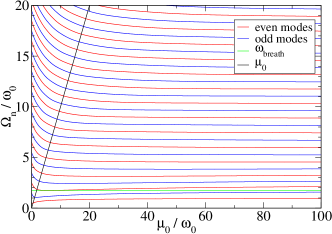
Figure 1: Frequencies of odd (blue) and even (red) excitations versus the chemical potential $\mu_{0}$ calculated using 100 harmonic oscillator basis functions. The frequencies equal the chemical potential at the intersection with the black line. The lowest odd mode converges for $\mu_{0}\to\infty$ to the classical Thomas-Fermi breathing frequency $\Omega_{\rm breath}^{\rm TF}=\sqrt{3}\omega_{0}$ (green), which follows from Eq. (3).

In Figure 1, the excitation frequencies $\Omega_{n}=\sqrt{A_{n}B_{n}}$ of the lowest modes are plotted versus the chemical potential $\mu_{0}$. For $\mu_{0}=0$, one has the equidistant spectrum of the harmonic oscillator $\Omega_{n}=(n+1/2)\omega_{0}$. Whereas for high $\mu_{0}\gg\Omega_{n}$, the frequencies become almost independent of the chemical potential. In particular, the frequency $\Omega_{1}$ of the lowest excitation with odd parity tends for $\mu_{0}\to\infty$ towards the Thomas-Fermi breathing frequency $\Omega_{\rm breath}^{\rm TF}=\sqrt{3}\omega_{0}$ obtained from Eq. (3).

The discrepancy between these two frequencies $\Omega_{1}$ and $\Omega_{\rm breath}^{\rm TF}$ for finite values of the chemical potential $\mu_{0}$ hints at shortcomings of the Thomas-Fermi approximation. In particular, Eq. (3) does not describe the breathing motion of the background properly and care must be taken when employing Eqs. (9) for the order parameter. Nonetheless, Eq. (3) still predicts the correct order of magnitude of the characteristic response time of the background, $1/\omega_{\rm breath}={\cal O}(1/\omega_{\rm breath}^{\rm TF})$, to variations of trap frequency or interaction strength.

Hence, it is still possible to discuss several cases, where the difference of $\omega_{\rm breath}$ and $\omega_{\rm breath}^{\rm TF}$ is either small or does not matter: firstly, if the shape of the condensate varies only slowly, i.e., if $\dot{b}\ll\omega_{\rm breath}$ and the condensate can adapt to changes of $\omega$ and/or $g$ immediately. Secondly, if no breathing oscillations are excited, e.g., because the condensate expands or contracts, see also Eqs. (35) and (36). And, thirdly, for very large chemical potentials, $\mu_{0}\to\infty$, the Thomas-Fermi approximation becomes exact. The quantum fluctuations are in the hydrodynamic regime and their effective evolution equations (28) decouple. In order to address cases where breathing of the background occurs, it would be necessary to abandon the Thomas-Fermi approximation (9) and to solve the Gross-Pitaevskii equation (6), which could, e.g., be done by expanding the order parameter $\psi_{0}$ into oscillator functions GP-modeexp .

V.2 Exponential sweep in stationary condensate

A stationary condensate, i.e., $b=1$, can be accomplished through simultaneous variation of trap frequency $\omega$ and interaction strength $g$, cf. Eq. (3)

$$f^{2}(t)\,=\,\frac{\omega^{2}(t)}{\omega_{0}^{2}}\,=\,\frac{g(t)}{g_{0}}\,,$$ (41)

though, one should be aware that this only holds within the Thomas-Fermi approximation: the instantaneous chemical potential must at all times be much larger than the trap frequency

$$\mu_{\rm inst}(t)\,=\,\mu_{0}f^{2}(t)\gg\omega(t)\,=\,\omega_{0}f(t)\,.$$ (42)

If both were of the same order, the kinetic term, $-\mbox{\boldmath$\nabla$}_{\bm{x}}^{2}\psi_{0}/2$, in the Gross-Pitaevskii equation (6) becomes important; no stationary background could be realized even for simultaneous variation of $\omega$ and $g$.

V.2.1 Analytical effective spacetime solution

For an exponential sweep

$$f^{2}(t)\,=\,e^{-2\gamma t}\,,\qquad\gamma\,>\,0\,,$$ (43)

the effective second-order equation (31) for the phase fluctuations in the hydrodynamic limit

$$\left[\frac{\partial^{2}}{\partial t^{2}}+4\gamma\frac{\partial}{\partial t}-f^{2}g_{0}\varrho_{0}\mbox{\boldmath$\nabla$}_{x}^{2}\right]\delta\hat{\phi}\,=\,0\,.$$ (44)

is that of a massless scalar field in a de Sitter spacetime with exponentially growing scale factor $a_{\rm FLRW}=1/f=e^{\gamma t}$, cf. Eq. (30) – which is believed to describe the universe during the epoch of cosmic inflation LL ; Wald . For the time-dependence (43), the integral (32) is finite and an effective sonic horizon occurs; the quantum fluctuations freeze and get amplified.

Instead of solving Eq. (44) for $\delta\hat{\phi}$, I will consider the evolution equation of the density fluctuations $\hat{X}_{n}^{+}$

$$\left[\frac{\partial^{2}}{\partial t^{2}}+\gamma^{2}e^{-2\gamma(t-t_{n})}\right]\hat{X}_{n}^{+}\,=\,0\,,$$ (45)

where $A_{n}B_{n}=\gamma^{2}e^{2\gamma t_{n}}$. Obviously, all modes undergo the same evolution just at different times. Eq. (45) can be solved analytically in terms of Bessel functions Abramowitz

$$\hat{X}_{n}^{+}\,=\,\sqrt{\frac{\pi B_{n}}{2\gamma}}\left\{\hat{a}_{n}H_{0}^{(1)}(e^{z})+\hat{a}_{n}^{\dagger}H_{0}^{(2)}(e^{z})\right\}\,.$$ (46)

where $z=-\gamma(t-t_{n})$. The Hankel functions $H_{0}^{(1/2)}$ have the proper asymptotics for early times $t\to-\infty$ such that the operators $\hat{a}_{n}$ annihilate the initial vacuum state. The phase fluctuations $\hat{X}_{n}^{-}=(1/2B_{n})\partial\hat{X}_{n}^{+}/\partial t$ read

$$\hat{X}_{n}^{-}\,=\,\sqrt{\frac{\pi\gamma}{8B_{n}}}\left\{\hat{a}_{n}e^{z}H_{1}^{(1)}(e^{z})+\hat{a}_{n}^{\dagger}e^{z}H_{1}^{(2)}(e^{z})\right\}\,.$$ (47)

From these expressions (46) and (47), I can infer the correlations of each mode. At late times follows

$$\left\langle(\hat{X}_{n}^{+})^{2}\right\rangle(t\to\infty)\, =\,\frac{2\gamma B_{n}}{\pi}(t-t_{n})^{2}\,,$$

$$\left\langle(\hat{X}_{n}^{-})^{2}\right\rangle(t\to\infty)\, =\,\frac{\gamma}{2\pi B_{n}}\,.$$ (48)

Comparison with the adiabatic values $\langle(\hat{X}_{n}^{\pm})^{2}\rangle_{\rm ad}$, cf. Eq. (73), yields the quasi-particle number at late times

$$N_{n}(t\to\infty)\,=\,\frac{1}{\pi}e^{\gamma(t-t_{n})}-1\,.$$ (49)

The occupation number of all modes grows exponentially though at different times $t-t_{n}$, where the shift $t_{n}$ is determined by the excitation frequencies $\sqrt{A_{n}B_{n}}=\gamma e^{\gamma t_{n}}$. However, one should bear in mind that Eq. (45) is only valid for a limited time before leaving the hydrodynamic regime.

V.2.2 Numerical results

In order to go beyond the effective space-time description and thus the analytical findings (46)-(49), I will now consider the full evolution equations (25). The sweep rate $\gamma=0.1$ shall be chosen such that all modes evolve adiabatically at first, i.e., $\gamma\ll\Omega_{n}(t_{\rm in})$ for all $n$. When subsequently reducing trap potential and coupling strength, the excitation frequencies $\Omega_{n}(t)$ decrease and non-adiabatic evolution sets in at different times for each mode. The fluctuations freeze and get amplified.

Figure 2 shows the instantaneous particle numbers of the lowest three modes for initial chemical potential $\mu_{0}=50$ and $\gamma=0.1$. The lowest excitation, $n=0$, which becomes non-adiabatic first, acquires the largest particle number. The next two modes, $n=1,2$, experience less squeezing, though, remarkably, $N_{2}>N_{1}$ – an unexpected result, which can be explained by the coupling of different modes: the second even mode, $n=2$, gets populated from the principle excitation, $n=0$, whereas the coupling matrix elements between $n=0$ and $n=1$ are zero because of different parity.

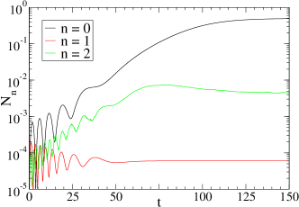
Figure 2: Instantaneous particle number in the lowest three quasi-particle modes for an exponential sweep (43). The initial chemical potential is $\mu_{0}=50$ and the sweep rate $\gamma=0.1$. At $t\approx 80$, the chemical potential equals the trap frequency. For the calculation of the eigenmodes $h_{n}^{\pm}$ and the coupling matrices (18), I used the harmonic oscillator functions $h_{\alpha}(x)$ up to $\alpha=79$, cf. Appendix III. The lowest 20 modes $\hat{X}_{n}^{\pm}$ were then propagated. The numerical accuracy was set to $10^{-6}$.

VI Summary

The main objective of this Article was the investigation of quantum fluctuations in time-dependent harmonically-trapped Bose-Einstein condensates with repulsive interactions. To this end, the linear fluctuations were expanded into their initial eigenmodes and the field equations were diagonalized. This diagonal form, however, persists only as long as the condensate is at rest; as soon as trap frequency or interaction strength are varied, the coupling of different modes sets in. (Only part of which can be accounted for by transforming to the instantaneous eigenmodes, though the definition of instantaneous eigenmodes is a non-trivial task.)

Two regimes were identified: firstly, for energies much smaller than the chemical potential, the coupling of different modes is negligible and an effective space-time metric might be introduced for the phase fluctuations. This, however, necessitates a redefinition of the time coordinate such that the required change of trap frequency and/or interaction strength for a certain dynamics of this effective space-time is not obvious. It turned out that the sole variation of the interaction coefficient $g(t)$ in a smooth monotonic way is hardly sufficient to render the evolution of the quantum fluctuations non-adiabatic, since the expansion/contraction of the background might compensate for changes of $g$ such that the sound velocity (in comoving coordinates) remains constant. Breathing oscillations of the background, excited, e.g., by the sudden change of the interaction coefficient $g$, might still yield a notable amount of quasi-particles. And secondly, if the excitation energy is of the same order as the chemical potential, different quasi-particle modes couple.

The amplification and freezing of the fluctuations and also the coupling of different modes was illustrated in an example, where the trap frequency and interaction strength were exponentially ramped down such that the shape of the condensate remains constant. For the considered parameters, a quasi-particle number of 0.5 was obtained in the lowest mode, though higher occupation numbers could be achieved by faster sweep rates or starting with a higher chemical potential. The inversion of the occupation number in the next two modes could be attributed to the inter-mode coupling: although the third excitation, $n=2$, experiences a much briefer period of non-adiabatic evolution than the second mode, $n=1$, only the former couples to the lowest mode, $n=0$, and gets populated from it.

Appendix A Eigenmodes

The aim of this Appendix is the derivation of the initial eigenfunctions $h_{n}^{\pm}$ of density and phase fluctuations. To this end, let me expand the field operator into any orthonormal basis $\{h_{\alpha}(\bm{x})\}$ of the underlying Hilbert space $L^{2}(\mathbb{R}^{D})$ with some operator-valued coefficients $\hat{\chi}_{\alpha}^{\pm}(t)$

$$\hat{\chi}_{\pm}(\bm{x},t)\,=\,h_{\alpha}(\bm{x})\hat{\chi}_{\alpha}^{\pm}(t)\,.$$ (50)

Lower-case Greek indices ($\alpha$, $\beta$,…) shall denote the components in this arbitrary basis, while lower-case Latin indices ($m$, $n$,…) label the initial eigenmodes.

If the condensate is initially at rest, the scale factor $b=1$ and the phase of the order parameter is homogenous $\mbox{\boldmath$\nabla$}_{\bm{x}}\phi_{0}=0$ such that $\mbox{\boldmath$v$}_{0}=0$ and thus $\mathcal{V}_{nm}=0$, cf. (19). The evolution equations (11) simplify considerably and can be expanded into the basis $\{h_{\alpha}\}$. It follows, cf. (17)

$$-2\frac{\partial}{\partial t}\hat{\chi}_{\alpha}^{-}\, =\,\mathcal{A}_{\alpha\beta}\hat{\chi}_{\beta}^{+}\, = \,\int d^{D}x\,h_{\alpha}\mathcal{K}_{+}h_{\beta}\hat{\chi}_{\beta}^{+}\,,$$

$$\frac{1}{2}\frac{\partial}{\partial t}\hat{\chi}_{\alpha}^{+}\, =\,\mathcal{B}_{\alpha\beta}\hat{\chi}_{\beta}^{-}\, = \,\int d^{D}x\,h_{\alpha}\mathcal{K}_{-}h_{\beta}\hat{\chi}_{\beta}^{-}\,,$$ (51)

where $\mathcal{K}_{\pm}$ are defined in Eq. (12). The matrices $\mathcal{A}_{\alpha\beta}$ and $\mathcal{B}_{\alpha\beta}$ are real and symmetric but do not commute due to $\left[\mathcal{K}_{+},\mathcal{K}_{-}\right]\neq 0$, cf. (13). From Eqs. (51), I obtain second-order evolution equations for phase and density fluctuations

$$\frac{\partial^{2}}{\partial t^{2}}\hat{\chi}_{\alpha}^{-}\, =\,-\mathcal{A}_{\alpha\beta}\mathcal{B}_{\beta\gamma}\hat{\chi}_{\gamma}^{-}\,,$$

$$\frac{\partial^{2}}{\partial t^{2}}\hat{\chi}_{\alpha}^{+}\, =\,-\mathcal{B}_{\alpha\beta}\mathcal{A}_{\beta\gamma}\hat{\chi}_{\gamma}^{+}\,,$$ (52)

which can be diagonalized by a transformation to the eigenvectors.

Because the matrix $\mathcal{A}_{\alpha\beta}\mathcal{B}_{\beta\gamma}\neq\mathcal{B}_{\alpha\beta}\mathcal{A}_{\beta\gamma}$ is not symmetric, phase and density fluctuations obey different eigenvalue equations

$$\mathcal{A}_{\alpha\beta}\mathcal{B}_{\beta\gamma} v_{\gamma}^{n}\, =\,\lambda_{n}v_{\alpha}^{n}\,,$$

$$\mathcal{B}_{\alpha\beta}\mathcal{A}_{\beta\gamma} \tilde{v}_{\gamma}^{n}\, =\,\tilde{\lambda}_{n}\tilde{v}_{\alpha}^{n}\,,$$ (53)

where $n$ denotes the vectors and $\alpha$ merely counts the components in the particular basis representation (50). For brevity, I will only discuss the eigenvectors of $\mathcal{A}\mathcal{B}$ in the following, though the same applies for those of $\mathcal{B}\mathcal{A}$ as well. The eigenvectors are generally not orthogonal

$$\sum_{\alpha}v_{\alpha}^{n}v_{\alpha}^{m}\, \neq\,\delta_{nm}\,,$$ (54)

but $\{v_{\alpha}^{n}\}$ usually still forms a basis. (Note, however, that the eigenvectors of a non-symmetric matrix not always span the entire vector space. But if the $v^{n}$ were no basis, the evolution equation (52) could not be diagonalized. This would mean that there existed some fluctuations, which have constant losses to some eigenmodes – rather unphysical in view of the stationary initial state considered here. Therefore, I will not discuss this case any further.) With the $v^{n}=h_{\alpha}v_{\alpha}^{n}$ forming a basis of $L^{2}(\mathbb{R}^{D})$, there must exist a dual basis $\{v^{{\rm d},n}\}$ in the space of linear functionals (the dual) on $L^{2}(\mathbb{R}^{D})$, which obeys

$$\int d^{D}x\,v^{{\rm d},n}v^{m}\,=\,\sum_{\alpha}v_{\alpha}^{{\rm d},n}v_{\alpha}^{m}\, =\,\delta_{nm}\,.$$ (55)

[Roughly speaking, the elements of $L^{2}(\mathbb{R}^{D})$ become column vectors in the basis expansion (50), whereas row vectors correspond to the functionals on $L^{2}(\mathbb{R}^{D})$, i.e., the elements of the dual. Since the eigenvectors $v^{n}$ form a basis, the matrix with the $v^{n}$ as columns must be invertible. The rows of the (left) inverse matrix then comprise the elements of the dual basis $\{v^{{\rm d},n}\}$ in the particular basis expansion (50).]

After the multiplication of the first of Eqs. (53) with $v_{\alpha}^{{\rm d},m}$ from the left and summation over $\alpha$ follows

$$v_{\alpha}^{{\rm d},m}\mathcal{A}_{\alpha\beta}\mathcal{B}_{\beta\gamma}v_{\gamma}^{n}\,=\,v_{\alpha}^{{\rm d},m}v_{\alpha}^{n}\lambda_{n}\,=\,\delta_{nm}\lambda_{m}\,,$$ (56)

which, because $\{v^{n}\}$ is a basis, implies that the $v^{{\rm d},n}$ are the left eigenvectors of $\mathcal{A}_{\alpha\beta}\mathcal{B}_{\beta\gamma}$ with the same eigenvalues $\lambda_{n}$

$$v_{\alpha}^{{\rm d},n}\mathcal{A}_{\alpha\beta}\mathcal{B}_{\beta\gamma}\, =\,v_{\gamma}^{{\rm d},n}\lambda_{n}\,.$$ (57)

Transposition yields

$$\mathcal{B}_{\gamma\beta}\mathcal{A}_{\beta\alpha}v_{\alpha}^{{\rm d},n}\, =\,\lambda_{n}v_{\gamma}^{{\rm d},n}\,.$$ (58)

i.e., the eigenvalue equation of $\mathcal{B}\mathcal{A}$, cf. (53). Hence, $\tilde{v}^{n}\propto v^{{\rm d},n}$ and $\mathcal{A}\mathcal{B}$ and $\mathcal{B}\mathcal{A}$ (i.e., density and phase fluctuations) must have the same spectrum $\{\lambda_{n}\}=\{\tilde{\lambda}_{n}\}$. For simplicity, $\tilde{v}^{n}=v^{{\rm d},n}$, which can be achieved by renormalization of $\tilde{v}^{n}$, in the following.

Note that the spectrum of a real non-symmetric matrix might contain pairs of complex conjugate eigenvalues $\lambda_{n}$, $\lambda_{n}^{*}$, which can be seen when taking the complex conjugate of (53). Complex eigenvalues $\Im\lambda_{n}\neq 0$ are associated with exponentially growing solutions, i.e., unstable modes. Since I am interested in the quantization of the stationary initial state, I will not discuss this case but instead assume $\lambda_{n}\in\mathbb{R}$ $\forall n$. (As can be easily verified, the components of the eigenvectors $v_{\alpha}^{n}$ and $\tilde{v}_{\alpha}^{n}$ must be real-valued as well.) Nonetheless, complex eigenvalues might still occur in dynamical situations, e.g., during the signature change event proposed in Silke or during (quantum) phase transitions Sachdev (see also Ref. spinor for an illustrative example).

The initial evolution equations (52) can be diagonalized by multiplication with the left eigenvectors

$$\frac{\partial^{2}}{\partial t^{2}}\tilde{v}_{\alpha}^{n}\hat{\chi}_{\alpha}^{-}\, =\,-\tilde{v}_{\alpha}^{n}\mathcal{A}_{\alpha\beta}\mathcal{B}_{\beta\gamma}\hat{\chi}_{\gamma}^{-}\, = \,-\lambda_{n}\tilde{v}_{\gamma}^{n}\hat{\chi}_{\gamma}^{-}\,,$$

$$\frac{\partial^{2}}{\partial t^{2}}v_{\alpha}^{n}\hat{\chi}_{\alpha}^{+}\, =\,-v_{\alpha}^{n}\mathcal{B}_{\alpha\beta}\mathcal{A}_{\beta\gamma}\hat{\chi}_{\gamma}^{+}\, = \,-\lambda_{n}v_{\gamma}^{n}\hat{\chi}_{\gamma}^{+}\,.$$ (59)

which leads to the definition of the density and phase fluctuation eigenmodes $\hat{X}_{n}^{\pm}$ through

$$\hat{X}_{n}^{-}\, =\,\tilde{v}_{\alpha}^{n}\hat{\chi}_{\alpha}^{-}\,,\quad \hat{X}_{n}^{+}\, =\,v_{\alpha}^{n}\hat{\chi}_{\alpha}^{+}\,,$$ (60)

where the spatial mode functions

$$h_{n}^{-}\,=\,v_{\alpha}^{n}h_{\alpha}\,,\quad h_{n}^{+}\,=\,\tilde{v}_{\alpha}^{n}h_{\alpha}\,.$$ (61)

follow from comparison of Eqs. (50) with (15) and the duality (55) of the $v_{\alpha}^{n}$ and $\tilde{v}_{\alpha}^{n}$ implies Eq. (16) for the $h_{n}^{\pm}$.

In view of (60), the initial evolution equations (51) can be transformed to the new basis, cf. Eq. (17)

$$-2\frac{\partial}{\partial t}\hat{X}_{n}^{-}\, =\,A_{n}\hat{X}_{n}^{+}\,,\quad\frac{1}{2}\frac{\partial}{\partial t}\hat{X}_{n}^{+}\, =\,B_{n}\hat{X}_{n}^{-}$$ (62)

where the transformed matrices

$$\mathcal{A}_{nm}\, =\,\tilde{v}_{\alpha}^{n}\mathcal{A}_{\alpha\beta}\tilde{v}_{\beta}^{m}\, =\,A_{n}\delta_{nm}\,,$$

$$\mathcal{B}_{nm}\, =\,v_{\alpha}^{n}\mathcal{B}_{\alpha\beta}v_{\beta}^{m}\, =\,B_{n}\delta_{nm}\,.$$ (63)

have become diagonal. Note that the transformation (60) is not orthogonal because the matrices comprising of the eigenvectors $v_{\alpha}^{n}$ and $\tilde{v}_{\alpha}^{n}$ are not orthogonal. Hence, the commutators are not preserved, in particular

$$\mathcal{A}_{\alpha\beta}\mathcal{B}_{\beta\gamma}\, \neq\,\mathcal{B}_{\alpha\beta}\mathcal{A}_{\beta\gamma}\,,$$

$$\mathcal{A}_{nm}\mathcal{B}_{ml}\, =\,\mathcal{B}_{nm}\mathcal{A}_{ml}$$ (64)

where the latter can be inferred from Eq. (56)

$$\lambda_{n}\delta_{nm}\, =\,\tilde{v}_{\alpha}^{n}\mathcal{A}_{\alpha\beta}\tilde{v}_{\beta}^{k}\,v_{\gamma}^{k}\mathcal{B}_{\gamma\delta}v_{\delta}^{m}\, = \,\mathcal{A}_{nk}\mathcal{B}_{km}\,=\,$$

$$(\lambda_{n}\delta_{nm})^{T}\, =\,v_{\alpha}^{n}\mathcal{B}_{\alpha\beta}v_{\beta}^{k}\,\tilde{v}_{\gamma}^{k}\mathcal{A}_{\gamma\delta}\tilde{v}_{\delta}^{m}\, = \,\mathcal{B}_{nk}\mathcal{A}_{km}\,.$$ (65)

Since $\mathcal{A}_{nm}$ and $\mathcal{B}_{nm}$ also commute with their product $\mathcal{A}_{nk}\mathcal{B}_{km}=\lambda_{n}\delta_{nm}$, which is diagonal, they must be diagonal, too.

Appendix B Observables

The duality condition (16) does not fix the norm of the eigenvectors but still permits the multiplication with an arbitrary factor $\Lambda_{n}$

$$h_{n}^{+} \to\Lambda_{n}h_{n}^{+}\,,\qquad h_{n}^{-} \to\frac{1}{\Lambda_{n}}h_{n}^{-}\,.$$ (66)

This renormalization then leads to a stretching/shrinking of the operator-valued coefficients, cf. (15)

$$\hat{X}_{n}^{+} \to\frac{1}{\Lambda_{n}}\hat{X}_{n}^{+}\,,\qquad \hat{X}_{n}^{-} \to\Lambda_{n}\hat{X}_{n}^{-}\,.$$ (67)

Since this is merely a basis transformation, the time-evolution of the quantum fluctuations $\hat{X}_{n}^{\pm}$ must be unaffected. To see this, recall the definitions (18) and (19) of the coupling matrices: they are the matrix elements of the operators $\mathcal{K}_{\pm}$ and of $\mbox{\boldmath$v$}_{0}\mbox{\boldmath$\nabla$}_{\bm{x}}+(\mbox{\boldmath$\nabla$}_{\bm{x}}\mbox{\boldmath$v$}_{0})/2$ with respect to the basis functions $h_{n}^{\pm}$ and thus acquire additional factors as well. As expected, all of these factors cancel such that the time-evolution remains unchanged. In particular, the eigenfrequencies are invariant $\Omega_{n}=\sqrt{A_{n}B_{n}}\to\sqrt{\Lambda_{n}^{2}A_{n}B_{n}/\Lambda_{n}^{2}}=\Omega_{n}$.

B.1 Correlation functions

Furthermore the observables should not depend on the particular normalization of the basis functions. The relative density-density correlations at time $t$ read

$$\frac{\langle\delta\hat{\varrho}(\bm{x})\delta\hat{\varrho}(\bm{x}^{\prime})\rangle}{\langle\hat{\varrho}(\bm{x})\rangle\langle\hat{\varrho}(\bm{x}^{\prime})\rangle}\, =\,\frac{h_{n;t}^{+}(\bm{x})h_{m;t}^{+}(\bm{x}^{\prime})}{\sqrt{\varrho_{0}(\bm{x})\varrho_{0}(\bm{x}^{\prime})}}\langle\hat{X}_{n;t}^{+}\hat{X}_{m;t}^{+}\rangle$$

$$=\,\frac{h_{n;t}^{+}(\bm{x})h_{m;t}^{+}(\bm{x}^{\prime})}{\sqrt{\varrho_{0}(\bm{x})\varrho_{0}(\bm{x}^{\prime})}}G_{n;t}^{k}\bar{G}_{m;t}^{k}$$ (68)

where I used the instantaneous eigenmode basis $h_{n;t}^{+}$, see Eq. (22). Obviously, the factors $\Lambda_{n}$ and $1/\Lambda_{n}$ contributed by $h_{n;t}^{+}$ and $\hat{X}_{n;t}$ cancel each other and the spatial correlations are independent of the normalization $\Lambda_{n}$. Similarly, the expression for the spatial phase-phase correlations

$$\langle\delta\hat{\phi}(\bm{x})\delta\hat{\phi}(\bm{x}^{\prime})\rangle\, =\,\frac{h_{n;t}^{-}(\bm{x})h_{m;t}^{-}(\bm{x}^{\prime})}{\sqrt{\varrho_{0}(\bm{x})\varrho_{0}(\bm{x}^{\prime})}}\langle\hat{X}_{n;t}^{-}\hat{X}_{m;t}^{-}\rangle$$

$$=\,\frac{h_{n;t}^{-}(\bm{x})h_{m;t}^{-}(\bm{x}^{\prime})}{\sqrt{\varrho_{0}(\bm{x})\varrho_{0}(\bm{x}^{\prime})}}F_{n;t}^{k}\bar{F}_{m;t}^{k}\,.$$ (69)

yields the same result regardless of the employed basis.

Hence, the factors $\Lambda_{n}$ can be chosen at will. There exist, however, several convenient choices for $\Lambda_{n}$: firstly, the density modes might be normalized to unity, $\int d^{D}x(h_{n}^{+})^{2}=1$. This is advantageous if left and right eigenvectors are the same, i.e., if $\mathcal{A}\mathcal{B}$ is symmetric. The drawback is that if $\mathcal{A}\mathcal{B}$ is not symmetric and therefore $h_{n}^{+}\neq h_{n}^{-}$, only one of the mode functions, $h_{n}^{+}$, can be normalized to unity, whereas the norm of the $h_{n}^{-}$ follows from Eq. (16). And, secondly, these factors $\Lambda_{n}$ can be fixed by demanding $A_{n}=B_{n}=\Omega_{n}$. In this case, the prefactors of (20) initially obey $F_{n}^{m}(t_{\rm in})=\delta_{nm}/\sqrt{2}$ and $G_{n}^{m}(t_{\rm in})=i\delta_{nm}/\sqrt{2}$ and both quadratures $\langle(\hat{X}_{n}^{\pm})^{2}\rangle(t_{\rm in})=1/2$. However, one should note that neither of the eigenfunctions $h_{n}^{\pm}$ is generally normalized to unity, $\int d^{D}x(h_{n}^{\pm})^{2}\neq 1$.

Of course, the coefficients $\langle\hat{X}_{n;t}^{+}\hat{X}_{m;t}^{+}\rangle$ and $\langle\hat{X}_{n;t}^{-}\hat{X}_{m;t}^{-}\rangle$ do depend on the particular choice of the basis functions $h_{n;t}^{\pm}$ and thus also on the factors $\Lambda_{n}$. For instance, the adiabatic density-density and phase-phase correlations of a particular mode read

$$\left\langle\hat{X}_{n;t}^{-}\hat{X}_{n;t}^{-}\right\rangle_{\rm ad}(t)\, =\,\frac{A_{n;t}}{2\Omega_{n;t}}\, \propto \,\frac{1}{\Lambda_{n}^{2}}\,,$$

$$\left\langle\hat{X}_{n;t}^{+}\hat{X}_{n;t}^{+}\right\rangle_{\rm ad}(t)\, =\,\frac{\Omega_{n;t}}{2A_{n;t}}\, \propto \,\Lambda_{n}^{2}\,.$$ (70)

The dependence on the factor $\Lambda_{n}$ becomes important regarding the low excitations in the Thomas-Fermi approximation, cf. Sec. IV: the modes decouple and it is not necessary to introduce a new spatial basis $h_{n}^{\pm}$ at the time of measurement. One has instead $A_{n;t}=f^{2}A_{n;t_{0}}$ and $B_{n;t}=B_{n;t_{0}}$ such that $\langle\hat{X}_{n;t}^{+}\hat{X}_{n;t}^{+}\rangle_{\rm ad}\propto f$ while $\langle\hat{X}_{n;t}^{-}\hat{X}_{n;t}^{-}\rangle_{\rm ad}\propto 1/f$, i.e., the phase and density fluctuations apparently increase or decrease even for adiabatic evolution. In view of this $\Lambda_{n}$ ambiguity, the (absolute) density-density or phase-phase correlations provide no adequate measure for the squeezing (i.e., non-adiabaticity) of a single mode. The Fourier transforms of Eqs. (68) and (69) on the other hand are independent of $\Lambda_{n}$ but do not represent the excitation eigenmodes.

B.2 Bogoliubov transformation and particle production

As will be shown in the following, the (instantaneous) quasi-particle number measures the relative deviation of density and phase fluctuations from their adiabatic values. In view of the different expansions (15) and (22) of density and phase fluctuations into their initial and adiabatic eigenfunctions, the corresponding creation and annihilation operators $\hat{a}_{n}^{\dagger}$, $\hat{a}_{n}$ and $\hat{b}_{n;t}^{\dagger}$, $\hat{b}_{n;t}$, respectively, can be transformed by virtue of a Bogoliubov transformation. For the annihilators $\hat{b}_{n;t}$ follows in particular

$$\hat{b}_{n;t}\, =\,\sqrt{\frac{\Omega_{n;t}}{2A_{n;t}}}\hat{X}_{n;t}^{-}-i\sqrt{\frac{A_{n;t}}{2\Omega_{n;t}}}\hat{X}_{n;t}^{+}$$

$$=\,\alpha_{nm}(t)\hat{a}_{m}+\beta_{nm}(t)\hat{a}_{m}^{\dagger}\,$$ (71)

with the Bogoliubov coefficients $\alpha_{nm}$ and $\beta_{nm}$. The first line follows from inversion of Eq. (24) and the second line can be inferred after transforming (20) to the new basis $h_{n;t}^{\pm}$. Since $\beta_{nm}\neq 0$ for non-adiabatic evolution, the quasi-particle number operator $\hat{N}_{n}(t)=\hat{b}_{n;t}^{\dagger}\hat{b}_{n;t}$ will have a non-zero expectation value as well

$$N_{n}(t)\, =\,\left\langle\hat{b}_{n;t}^{\dagger}\hat{b}_{n;t}\right\rangle\,=\,\sum_{m}|\beta_{nm}(t)|^{2}$$

$$=\ \frac{\Omega_{n;t}}{2A_{n;t}}\left\langle(\hat{X}_{n;t}^{-})^{2}\right\rangle+\frac{A_{n;t}}{2\Omega_{n;t}}\left\langle(\hat{X}_{n;t}^{+})^{2}\right\rangle$$

$$\qquad+\frac{i}{2}\left\langle\left[\hat{X}_{n;t}^{+},\hat{X}_{n;t}^{-}\right]\right\rangle$$ (72)

where the commutator $\left[\hat{X}_{n;t}^{+},\hat{X}_{n;t}^{-}\right]=-i$. Noting that the prefactors $\Omega_{n;t}/2A_{n;t}$ and $A_{n;t}/2\Omega_{n;t}$ are just the adiabatic density-density and phase-phase correlations, see Eq. (70), the particle number can be rewritten

$$N_{n}(t)\, =\,\frac{\langle(\hat{X}_{n;t}^{-})^{2}\rangle-\frac{A_{n;t}}{2\Omega_{n;t}}}{2A_{n;t}/\Omega_{n;t}}+\frac{\langle(\hat{X}_{n;t}^{+})^{2}\rangle-\frac{\Omega_{n;t}}{2A_{n;t}}}{2\Omega_{n;t}/A_{n;t}}\,,$$ (73)

i.e., the instantaneous particle number gives just the relative deviation of the density and phase correlations from their adiabatic values. Note that expression (73) does not contain the correlations between different modes. To this end, it would be necessary to evaluate $\langle\hat{N}_{n}\hat{N}_{m}\rangle$, which is fourth order in the $\hat{b}_{n;t}$. This observable can be reduced to expectation values quadratic in in the $\hat{b}_{n;t}$ by virtue of Wick’s theorem, see, e.g., Giorgini2 .

B.3 Scaling

Another interesting aspect regards the scaling of the correlation functions (68) and (69) with the interaction strength: within the Thomas-Fermi approximation, see Sec. IV, the evolution equations (25) are independent of $g_{0}$. All properties of the linear excitations are determined by the chemical potential $\mu_{0}$ and the variations $g(t)/g_{0}$ and $\omega(t)/\omega_{0}$, in particular the expectation values $\langle\hat{X}_{n;t}^{\pm}\hat{X}_{m;t}^{\pm}\rangle$. Only the normalization factor $\sqrt{\varrho_{0}(\bm{x})\varrho_{0}(\bm{x}^{\prime})}=(1/g_{0})\sqrt{[\mu-V(\bm{x})][\mu_{0}-V(\bm{x}^{\prime})]}$ in Eqs. (68) and (69) depends on $g_{0}$. Hence, the relative density-density and phase-phase correlations in the Thomas-Fermi approximation are both proportional to $g_{0}$ for fixed $\mu_{0}$.

References

• (1) I. Bloch, J. Dalibard, and W. Zwerger, Rev. Mod. Phys. 80, 885 (2008).
• (2) L. Pitaevskii and S. Stringari, Bose-Einstein Condensation (Oxford University Press, Oxford, UK, 2003); A. J. Leggett, Rev. Mod. Phys. 73, 307 (2001).
• (3) M. Greiner et al., Nature 415, 39 (2002); F. Gerbier et al., Phys. Rev. Lett. 96, 090401 (2006); S. Fölling et al., Phys. Rev. Lett. 97, 060403 (2006).
• (4) M. P. A. Fisher, P. B. Weichman, G. Grinstein, and D. S. Fisher, Phys. Rev. B 40, 546 (1989); D. Jaksch et al., Phys. Rev. Lett. 81, 3108 (1998); D. Jaksch and P. Zoller, Ann. Phys. (N.Y.) 315, 52 (2005); R. Schützhold, M. Uhlmann, Y. Xu, and U. R. Fischer, Phys. Rev. Lett. 97, 200601 (2006); C. Kollath, A. M. Läuchli, and E. Altman, Phys. Rev. Lett. 98, 180601 (2007).
• (5) G. Volovik, The Universe in a Helium Droplet (Oxford University Press, Oxford, UK, 2003).
• (6) C. Barceló, S. Liberati, and M. Visser, Living Rev. Relativity 8, 12 (2005).
• (7) U. R. Fischer, Mod. Phys. Lett. A 19, 1789 (2004).
• (8) P. Jain, S. Weinfurtner, M. Visser, and C. W. Gardiner, Phys. Rev. A 76, 033616 (2007).
• (9) S. Weinfurtner, A. White, and M. Visser, Phys. Rev. D 76, 124008 (2007).
• (10) C. Barceló, S. Liberati, and M. Visser, Phys. Rev. A 68, 053613 (2003); C. Barceló, S. Liberati, and M. Visser, Int. J. Mod. Phys. D 12, 1641 (2003); C. Barceló, S. Liberati, and M. Visser, Class. Quant. Grav. 18, 1137 (2001); ibid. 18, 3595 (2001).
• (11) U. R. Fischer and R. Schützhold, Phys. Rev. A 70, 063615 (2004).
• (12) M. Uhlmann, Yan Xu, and R. Schützhold, New J. Phys. 7, 248 (2005).
• (13) P. O. Fedichev and U. R. Fischer, Phys. Rev. A 69, 033602 (2004).
• (14) Y. Kurita and T. Morinari, Phys. Rev. A 76, 053603 (2007).
• (15) M. Visser and S. Weinfurtner, Phys. Rev. D 72, 044020 (2005).
• (16) L. J. Garay, J. R. Anglin, J. I. Cirac, and P. Zoller, Phys. Rev. Lett. 85, 4643 (2000)
• (17) S. Wüster, Phys. Rev. A 78, 021601(R) (2008); S. Wüster and C. M. Savage, Phys. Rev. A 76, 013608 (2007).
• (18) W. G. Unruh, Phys. Rev. Lett. 46, 1351 (1981); W. G. Unruh, Phys. Rev. D 51, 2827 (1995).
• (19) M. Novello, M. Visser, and G. Volovik (eds.), Artificial Black Holes (World Scientific, Singapore, 2002).
• (20) S. W. Hawking, Nature 248, 30 (1974); S. W. Hawking, Commun. math. Phys. 43, 199 (1975).
• (21) A. R. Liddle and D. H. Lyth, Cosmological Inflation and Large-Scale Structure, (Cambridge University Press, Cambridge, UK, 2000).
• (22) N. D. Birrell and P. C. Q. Davies, Quantum Fields in Curved Space (Cambridge University Press, Cambridge, UK, 1982).
• (23) S. Fölling, et al., Nature 434, 481 (2005).
• (24) D. Hellweg et al., Phys. Rev. Lett. 91, 010406 (2003); S. Hofferberth et al., Nature 449, 324 (2007); Nature Phys. 4, 489 (2008).
• (25) S. B. Papp et al., preprint arXiv:0805.0295.
• (26) M. Schellekens et al., Science 310, 648 (2005).
• (27) J. Esteve et al., Phys. Rev. Lett. 96, 130403 (2006).
• (28) A. Griffin, Phys. Rev. B 53, 9341 (1996); S. Giorgini Phys. Rev. A 61, 063615 (2000).
• (29) M. J. Davis, S. A. Morgan, and K. Burnett, Phys. Rev. Lett. 87, 160402 (2001); P. B. Blakie and M. J. Davis, Phys. Rev. A 72, 063608 (2005); P. B. Blakie et al., preprint arXiv:0809.1487.
• (30) S. Wüster, J. J. Hope, and C. M. Savage, Phys. Rev. A 71, 033604 (2005); S. Wüster et al., Phys. Rev. A 75, 043611 (2007).
• (31) Dimensionless units can be introduced through the initial trap frequency $\omega_{0}$ and the atom mass $m$. All energies are then measured in units of $\omega_{0}$, the dimensionless time is defined through $t=\omega_{0}\tau$, and the characteristic length $a_{0}=1/\sqrt{m\omega_{0}}$, where $\hbar=1$.
• (32) E. Tiesinga, B. J. Verhaar, and H. T. C. Stoof Phys. Rev. A 47, 4114 (1993); S. Inouye et al., Nature 392, 151 (1998); Ph. Courteille, R. S. Freeland, and D. J. Heinzen, Phys. Rev. Lett. 81, 69 (1998).
• (33) Y. Castin and R. Dum, Phys. Rev. Lett. 77, 5315 (1996); Yu. Kagan, E. L. Surkov, and G. V. Shlyapnikov, Phys. Rev. A 54, R1753 (1996).
• (34) M. Girardeau and R. Arnowitt, Phys. Rev. 113, 755(1959); C. W. Gardiner, Phys. Rev. A 56, 1414, (1997); M. D. Girardeau, ibid 58, 775 (1998).
• (35) E. P. Gross, Nuovo Cimento 20, 454 (1961); L. P. Pitaevskii, Zh. Eksp. Teor. Fiz. 40, 646 (1961) [Sov. Phys. JETP 13, 451 (1961)].
• (36) N. N. Bogoliubov, J. Phys. (Moscow), 11, 23, (1947); P. G. de Gennes, Superconductivity of Metals and Alloys (W. A. Benjamin, New York, 1966).
• (37) As similar expansion of the linear fluctuations is also considered in Fetter . There, the authors expand the linear field operator $\hat{\chi}$ of a static/stationary condensate into eigenmodes and not the phase and density fluctuations $\hat{\chi}_{\pm}$. This leads to complex mode functions $v_{n}$ and $u_{n}$, while $h_{n}^{\pm}$ are real.
• (38) A. L. Fetter, Ann. Phys. (N.Y.) 70, 67 (1972); M. Lewenstein and L. You, Phys. Rev. Lett. 77, 3489 (1996); M. Naraschewski and R. J. Glauber, Phys. Rev. A 59, 4595 (1999).
• (39) R. Schützhold, Phys. Rev. Lett. 97, 190405 (2006).
• (40) The eigenfunctions of density and phase fluctuations $\delta\hat{\varrho}$ and $\delta\hat{\phi}$ are defined slightly differently than those of $\hat{\chi}_{\pm}$
$\displaystyle\hat{\chi}_{+}\,$ $\displaystyle=\,h_{n}^{+}\hat{X}_{n}^{+}\,$ $\displaystyle=$ $\displaystyle\,\frac{h_{n}^{\varrho}}{\sqrt{\varrho_{0}}}\delta\hat{\varrho}_{n}\,$ $\displaystyle=$ $\displaystyle\,\frac{\delta\hat{\varrho}}{\sqrt{\varrho_{0}}}$
$\displaystyle\hat{\chi}_{-}\,$ $\displaystyle=\,h_{n}^{-}\hat{X}_{n}^{-}\,$ $\displaystyle=$ $\displaystyle\,\sqrt{\varrho_{0}}h_{n}^{\phi}\delta\hat{\phi}\,$ $\displaystyle=$ $\displaystyle\,\sqrt{\varrho_{0}}\delta\hat{\phi}\,.$
Noting that $\mbox{\boldmath$\nabla$}_{x}\varrho_{0}\approx 0$ the center of the trap, the eigenfunctions $h_{n}^{+}$ and $h_{n}^{\varrho}$ (and similarly $h_{n}^{-}$ and $h_{n}^{\phi}$) must be approximately proportional for low excitations. Hence, the $X_{n}^{\pm}$ for $\Omega_{n}\ll\mu_{0}$ indeed represent the proper density and phase eigenmodes $\delta\hat{\varrho}_{n}$ and $\delta\hat{\phi}_{n}$ up to a constant prefactor $\varrho_{0}^{\pm 1/2}$.
• (41) R. M. Wald, General Relativity (University of Chicago Press, Chicago, IL, 1984).
• (42) C. W. Misner, K. S. Thorne, and J. A. Wheeler, Gravitation (W.H. Freeman, San Francisco, USA, 1973).
• (43) M. Visser Lorentzian Wormholes: From Einstein to Hawking (Springer, New York, 1996).
• (44) S. W. Hawking and G. F. R. Ellis, The Large Scale Structure of Spacetime (Cambridge University Press, Cambridge, UK, 1973).
• (45) M. Visser, Class. Quant. Grav. 15, 1767 (1998).
• (46) R. Schützhold, Lect. Notes Phys. 718, 5 (2007); Class. Quant. Grav. 25, 114011 (2008).
• (47) C. M. Dion and E. Cancès, Phys. Rev. E 67, 046706 (2003).
• (48) Handbook of Mathematical Functions, edited by M. Abramowitz and I. A. Stegun, (Dover, New York, 1970).
• (49) S. Sachdev, Quantum Phase Transitions (Cambridge University Press, Cambridge, UK, 2000).
• (50) L. E. Sadler et al., Nature 443, 312 (2006); H. Saito and M. Ueda, Phys. Rev. A 72, 023610 (2005); H. Saito, Y. Kawaguchi, and M. Ueda, Phys. Rev. Lett. 96, 065302 (2006); A. Lamacraft Phys. Rev. Lett. 98, 160404 (2007); M. Uhlmann, R. Schützhold, and U. R. Fischer, Phys. Rev. Lett. 99, 120407 (2007).
• (51) S. Giorgini, L. P. Pitaevskii, and S. Stringari, Phys. Rev. Lett. 80, 5040 (1998).