Graphical description of local Gaussian operations for continuous-variable weighted graph states

Abstract

The form of a local Clifford (LC, also called local Gaussian (LG)) operation for the continuous-variable (CV) weighted graph states is presented in this paper, which is the counterpart of the LC operation of local complementation for qubit graph states. The novel property of the CV weighted graph states is shown, which can be expressed by the stabilizer formalism. It is distinctively different from the qubit weighted graph states, which can not be expressed by the stabilizer formalism. The corresponding graph rule, stated in purely graph theoretical terms, is described, which completely characterizes the evolution of CV weighted graph states under this LC operation. This LC operation may be applied repeatedly on a CV weighted graph state, which can generate the infinite LC equivalent graph states of this graph state. This work is an important step to characterize the LC equivalence class of CV weighted graph states.

Graph states one ; two - or equivalently called stabilizer states, are special instances of multiparty quantum sates that are of interest in a number of domains in quantum information theory and quantum computation. Graph states can be defined in terms of the stabilizer formalism, which is a group-theoretic framework originally designed to construct broad classes of quantum error-correcting codes - the stabilizer codes three . In addition to their role in quantum error-correction, graph states have been used in a number of interesting applications, where the measure-based model of quantum computation known as the one-way quantum computer is certainly among the most prominent four .

Most of the concepts of quantum information and computation have been initially developed for discrete quantum variables, in particular two-level or spin-$\frac{1}{2}$ quantum variables (qubits). In parallel, quantum variables with a continuous spectrum, have attracted a lot of interest and appear to yield very promising perspectives concerning both experimental realizations and general theoretical insights five ; six , due to relative simplicity and high efficiency in the generation, manipulation, and detection of continuous variable (CV) state. CV cluster and graph states have been proposed seven , which can be generated by squeezed state and linear optics seven ; eight ; nine , and demonstrated experimentally for the four-mode cluster state ten ; eleven . The one-way CV quantum computation was also proposed with the CV cluster state twelve . Moreover, the protocol of CV anyonic statistics implemented with CV graph states is proposed thirteen .

It is well known that many graph states exhibit a high degree of genuine multi-party entanglement forteen , and that this entanglement is a key ingredient responsible for the successful use of these states in various applications. Therefore, a detailed study of the entanglement properties of graph states is of natural interest. The study of the nonlocal properties of graph states naturally leads to an investigation of the action of local unitary (LU) operations on graph states, and a classification of graph sates under LU equivalence. Especially, a subclass of LU operations known as local Clifford (LC) plays an important role. Due to the close connection between the Pauli group, the stabilizer formalism and the local Clifford group, the action of LC operation on graph states can be described efficiently. Recently, the action of LC operations on qubit graph states can entirely be understood in terms of a single elementary graph transformation rule, called the local complement rule fifteen ; one . A systematic classification of LC equivalence of graph states has been executed one . An efficient algorithm (i.e., with polynomial time complexity in the number of qubits) to decide whether two given stabilizer states are LC equivalent, is known sixteen . LU-LC equivalence problem still was a long-standing open problem in quantum information theory, which achieved the progress recently sixteen1 .

In the regime of continuous variable, LC equivalence of CV graph states just began to be studied very recently. The local complement rule was extended to the associated graphs of CV unweighted graph states seventeen . The simplest phenomenon was discussed seventeen , in which the corresponding LC operation was presented for the local complementation on four-mode unweighted graphs. It was shown that the corresponding LC operation for the local complementation can not exactly mirror that for qubit, which is not a single form compared with qubit. This result shows the complexity of CV quantum systems. Whether the local complementation for CV unweighted graphs can be implemented completely by the LC transformations and the general form of the corresponding LC operation can be found are still open question. In this paper, we consider another way to investigate LC operation of CV graph states as shown in Fig.1. First, the corresponding LC operation of local complementation for qubit graph states is generalized to CV graph states. Second, the CV weighted graph states is defined, which can be expressed by the stabilizer formalism in terms of generators within the Pauli group. It is distinctively different from the qubit weighted graph states, which can not be expressed by the stabilizer formalism forteen . The action of this LC operation on the CV weighted graph states is described by the graph rule. Thus, the successive application of this LC operation can generate the LC equivalence class of a CV weighted graph state with the infinite elements. It is worth remarking that, whether the whole LC equivalence class of a CV weighted graph state can be obtained by repeatedly applying this LC operation, still need be further investigated. In other words, what is the whole LC equivalence class of a CV weighted graph state and how achieve it by LC operations?

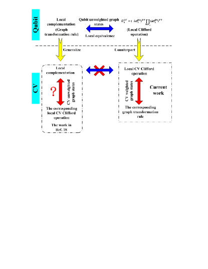
Figure 1: (Color online). The diagram describing the LC equivalence problem for qubit and CV graph states.

First, the CV operations eighteen are presented briefly in the follow. For CV, the Weyl-Heisenberg group, which is the group of phase-space displacements, is a Lie group with generators $\hat{x}=(\hat{a}+\hat{a}^{\dagger})/\sqrt{2}$ (quadrature-amplitude or position) and $\hat{p}=-i(\hat{a}-\hat{a}^{\dagger})/\sqrt{2}$ (quadrature-phase or momentum) of the electromagnetic field. These operators satisfy the canonical commutation relation $[\hat{x},\hat{p}]=i$ (with $\hbar=1$). The single mode Pauli operators are defined as $X(s)=exp[-is\hat{p}]$ and $Z(t)=exp[it\hat{x}]$ with $s,t\in\mathbb{R}$. These operators are non-commutative and obey the identity $X(s)Z(t)=e^{-ist}Z(t)X(s)$. In the Heisenberg picture, applying a Hamitonian $H$ gives a time evolution for operators $\dot{A}=i[H,A]$, so that $A(t)=exp[iHt]A(0)exp[-iHt]$. Accordingly, applying the Hamitonian $H=\hat{x}$ for time $t$ takes $\hat{x}\rightarrow\hat{x},\hat{p}\rightarrow\hat{p}-t$, and applying $H=-\hat{p}$ for time $s$ takes $\hat{x}\rightarrow\hat{x}-s,\hat{p}\rightarrow\hat{p}$. The Pauli operator $X(s)$ is a position-translation operator, which acts on the computational basis of position eigenstates as $X(s)|q\rangle=|q+s\rangle$, whereas $Z$ is a momentum-translation operator, which acts on the momentum eigenstates as $Z(t)|p\rangle=|p+t\rangle$. The transformation of the Pauli operators on the basis of position (momentum) eigenstates may be derived as follows. Let $\hat{x}^{\prime}=X(s)\hat{x}X(-s)=\hat{x}-s$, and consider $\hat{x}^{\prime}|q\rangle$. On the one hand, it must be $\hat{x}^{\prime}|q\rangle=(\hat{x}-s)|q\rangle=(q-s)|q\rangle$. On the other hand, it also is $\hat{x}^{\prime}|q\rangle=X(s)\hat{x}X(-s)|q\rangle=X(s)\hat{x}|q-s\rangle=(q-s)X(s)|q-s\rangle=(q-s)|q\rangle$. Thus $X(s)|q\rangle=|q+s\rangle$ is the correct operation. Similarly, it may be shown that $Z(t)|p\rangle=|p+t\rangle$ is also the correct transformation. The Pauli operators for one mode can be used to construct a set of Pauli operators $\{X_{i}(s_{i}),Z_{i}(t_{i});i=1,...,n\}$ for n-mode systems. This set generates the Pauli group $\mathcal{C}_{1}$. The clifford group $\mathcal{C}_{2}$ is the normalizer of the Pauli group, whose transformations acting by conjugating, preserve the Pauli group $\mathcal{C}_{1}$; i.e., a gate U is in the Clifford group if $\emph{UR}\emph{U}^{-1}\in\mathcal{C}_{1}$ for every $\emph{R}\in\mathcal{C}_{1}$. The Clifford group $\mathcal{C}_{2}$ for CV is shown eighteen to be the (semidirect) product of the Pauli group and linear symplectic group of all one-mode and two-mode squeezing transformations. Transformation between the position and momentum basis is given by the Fourier transform operator $F=exp[i(\pi/4)(\hat{x}^{2}+\hat{p}^{2})]$, with $F|q\rangle_{x}=|q\rangle_{p}$. This is the generalization of the Hadamard gate for qubits. The phase gate $P(\eta)=exp[i(\eta/2)\hat{x}^{2}]$ with $\eta\in\mathbb{R}$ is a squeezing operation for CV and the action $P(\eta)RP^{-1}(\eta)$ on the Pauli operators is

$$P(\eta):X(s) \rightarrow e^{-is^{2}\eta/2}Z(s\eta)X(s),$$

$$Z(t) \rightarrow Z(t),$$ (1)

in analogy to the phase gate of qubit. The controlled operation C-Z is generalized to controlled-$Z(C_{Z})$. This gate $C_{Z}=exp[i\hat{x}_{1}\bigotimes\hat{x}_{2}]$ provides the basic interaction for two mode 1 and 2, and describes the quantum nondemolition (QND) interaction. This set $\{X(s),F,P(\eta),C-Z;s,\eta\in\mathbb{R}\}$ generates the Clifford group. Here the controlled operation with any interaction strength $C_{Z}(\Omega)=exp[i\Omega\hat{x}_{1}\bigotimes\hat{x}_{2}]$ ($\Omega\in\mathbb{R}$) will be used in the following. Another type of the phase gate will also be utilized $P_{X}(\eta)=FP(\eta)F^{-1}=exp[i(\eta/2)\hat{p}^{2}]$ and the action on the Pauli operators is

$$P_{X}(\eta):X(s) \rightarrow X(s),$$

$$Z(t) \rightarrow e^{-it^{2}\eta/2}X(-t\eta)Z(t),$$ (2)

where $P_{X}(\eta)^{\dagger}=P_{X}(\eta)^{-1}=P_{X}(-\eta)$.

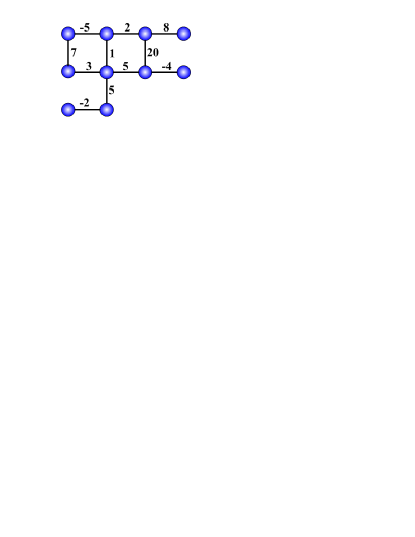
Figure 2: (Color online). Example for depicting the CV weighted graph state.

A weighted graph quantum state is described by a mathematical graph $G=(V,E)$, i.e. a finite set of $n$ vertices $V$ connected by a set of edges $E$ forteen , in which every edge is specified by a factor $\Omega_{ab}$ corresponding to the strength the modes a and b have interacted as shown Fig.2. The preparation procedure of CV weighted graph states is only to use the Clifford operations: first, prepare each mode (or graph vertex) in a phase-squeezed state, approximating a zero-phase eigenstate (analog of Pauli-X eigenstates), then, apply the QND coupling ($C_{Z}(\Omega)$) with the differen interaction strength $\Omega_{jk}$ to each pair of modes $(j,k)$ linked by a weighted edge in the graph. Note that CV unweighted graph states is to use the QND interaction all with the same strength. Since all C-Z gates commute, the resulting CV graph state becomes, in the limit of infinite squeezing, $g_{a}=(\hat{p}_{a}-\sum_{b\in N_{a}}\Omega_{ab}\hat{x}_{b})\rightarrow 0$, where the modes $a\in V$ correspond to the vertices of the graph of $n$ modes, while the modes $b\in N_{a}$ are the nearest neighbors of mode $a$. This relation is as a simultaneous zero-eigenstate of the position-momentum linear combination operators. The corresponding $n$ independent stabilizers for CV weighted graph states are expressed by $G_{a}(\xi)=exp[-i\xi g_{a}]=X_{a}(\xi)\prod_{b\in N_{a}}Z_{b}(\Omega_{ab}\xi)$ with $\xi\in\mathbb{R}$. Note that it is distinctively different from the qubit weighted graph states, which can not be expressed by the stabilizer formalism forteen . The main reason induced this difference is that the C-Z gate for qubit is periodic as a function of the interaction strength, however, the CV C-Z gate is not.

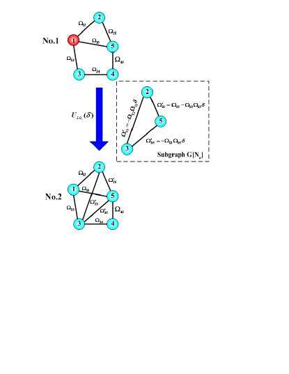
Figure 3: (Color online). Example of the graph rule of the LG operation $U_{LG_{1}}$ applied on a CV weighted graph state.

The action of the local complement as the graph rule, can be described as: letting $G=(V,E)$ be a graph and $a\in V$ be a vertex, the local complement of $G$ for $a$, denoted by $\lambda_{a}(G)$, is obtained by complementing the subgraph of $G$ generated by the neighborhood $N_{a}$ of $a$ and leaving the rest of the graph unchanged. The successive application of this rule suffices to generate the complete orbit of any qubit graph states. The corresponding LC operation of local complement for the qubit graph states is a single and simple form, which is expressed by $U_{a}^{LC}=(-i\sigma_{x}^{(a)})^{1/2}\prod_{b\in N_{a}}(i\sigma_{z}^{(b)})^{1/2}$ fifteen ; one . This formalism may be straightforward to generalize to CV weighted graph state, which is expressed by

$$U_{LG_{a}}(\delta)=P_{Xa}(-\delta)\prod_{b\in N_{a}}P_{b}(\Omega_{ab}^{2}\delta).$$ (3)

Now the action of this LC operation on CV weighted graph states is translated into transformations on their associated graphs, that is, to derive transformations rules, stated in purely graph theoretical terms, which completely characterize the evolution of CV weighted graph states under this LC operation. The graph rule of applying this LC operation is described as: first obtain the subgraph of $G$ generated by the neighborhood $N_{a}$ of $a$, then reset the weight factor of all edges of this subgraph calculated with the equation $\Omega_{b_{i}b_{j}}^{\prime}=\Omega_{b_{i}b_{j}}-\Omega_{ab_{i}}\Omega_{ab_{j}}\delta$, at last delete all the edges with the weight factor of zero, and leave the rest of the graph unchanged. Here, a subgraph $G[C]$ of a graph $G=(V,E)$, where $C\subset V$, is obtained by deleting all vertices and the incident edges that are not contained in $C$. Figure 3 presents an example of this graph rule applied on a CV weighted graph state. The five independent stabilizers of the weighted graph state No.1 $|\psi^{(1)}\rangle$ are given by

$$G_{1}^{(1)}(\xi) = X_{1}(\xi)Z_{2}(\Omega_{12}\xi)Z_{3}(\Omega_{13}\xi)Z_{5}(\Omega_{15}\xi),$$

$$G_{2}^{(1)}(\xi) = X_{2}(\xi)Z_{1}(\Omega_{12}\xi)Z_{5}(\Omega_{25}\xi),$$

$$G_{3}^{(1)}(\xi) = X_{3}(\xi)Z_{1}(\Omega_{13}\xi)Z_{4}(\Omega_{34}\xi),$$

$$G_{4}^{(1)}(\xi) = X_{4}(\xi)Z_{3}(\Omega_{34}\xi)Z_{5}(\Omega_{45}\xi),$$

$$G_{5}^{(1)}(\xi) = X_{5}(\xi)Z_{1}(\Omega_{15}\xi)Z_{2}(\Omega_{25}\xi)Z_{4}(\Omega_{45}\xi),$$ (4)

with $G_{i}^{(1)}(\xi)|\psi^{(1)}\rangle=|\psi^{(1)}\rangle$ in the limit of infinite squeezing, where $i=1,...,5$. Applying the LC operation $U_{LG_{1}}(\delta)$ to the vertex 1, the five independent stabilizers of the resulting graph state $|\psi^{(2)}\rangle=U_{LG_{1}}(\delta)|\psi^{(1)}\rangle$ are calculated by Eqs. 1,2,3,4 and with the relationship $U_{LG_{1}}(\delta)G_{1}^{(1)}(\xi)=G_{1}^{(1)}(\xi)U_{LG_{1}}(\delta)$, for example calculating $G_{2}^{(2)}(\xi)$,

$$|\psi^{(2)}\rangle = U_{LG_{1}}(\delta)G_{2}^{(1)}(\xi)U_{LG_{1}}^{-1}(\delta)U_{LG_{1}}(\delta)|\psi^{(1)}\rangle$$ (5)

$$= [e^{-i\xi^{2}\delta\Omega_{12}^{2}/2}Z_{2}(\delta\Omega_{12}^{2}\xi)X_{2}(\xi)]\times$$

$$[e^{i(\Omega_{12}\xi)^{2}\delta/2}X_{1}(\delta\Omega_{12}\xi)Z_{1}(\Omega_{12}\xi)]\times$$

$$Z_{5}(\Omega_{25}\xi)U_{LG_{1}}(\delta)|\psi^{(1)}\rangle$$

$$= X_{2}(\xi)Z_{1}(\Omega_{12}\xi)Z_{5}(\Omega_{25}\xi)[X_{1}(\delta\Omega_{12}\xi)Z_{2}(\delta\Omega_{12}^{2}\xi)]\times$$

$$U_{LG_{1}}(\delta)G_{1}^{(1)}(-\delta\Omega_{12}\xi)|\psi^{(1)}\rangle$$

$$= X_{2}(\xi)Z_{1}(\Omega_{12}\xi)Z_{3}(-\Omega_{12}\Omega_{13}\delta\xi)\times$$

$$Z_{5}((\Omega_{25}-\Omega_{12}\Omega_{15}\delta)\xi)|\psi^{(2)}\rangle$$

$$= G_{2}^{(2)}(\xi)|\psi^{(2)}\rangle$$

to obtain

$$G_{1}^{(2)}(\xi) = X_{1}(\xi)Z_{2}(\Omega_{12}\xi)Z_{3}(\Omega_{13}\xi)Z_{5}(\Omega_{15}\xi),$$

$$G_{2}^{(2)}(\xi) = X_{2}(\xi)Z_{1}(\Omega_{12}\xi)Z_{3}(-\Omega_{12}\Omega_{13}\delta\xi)$$

$$Z_{5}((\Omega_{25}-\Omega_{12}\Omega_{15}\delta)\xi)$$

$$= X_{2}(\xi)Z_{1}(\Omega_{12}\xi)Z_{3}(\Omega_{23}^{\prime}\xi)Z_{5}(\Omega_{25}^{\prime}\xi),$$

$$G_{3}^{(2)}(\xi) = X_{3}(\xi)Z_{1}(\Omega_{13}\xi)Z_{2}(\Omega_{23}^{\prime}\xi)Z_{4}(\Omega_{34}\xi)Z_{5}(\Omega_{35}^{\prime}\xi),$$

$$G_{4}^{(2)}(\xi) = X_{4}(\xi)Z_{3}(\Omega_{34}\xi)Z_{5}(\Omega_{45}\xi),$$

$$G_{5}^{(2)}(\xi) = X_{5}(\xi)Z_{1}(\Omega_{15}\xi)Z_{2}(\Omega_{25}^{\prime}\xi)Z_{3}(\Omega_{35}^{\prime}\xi)Z_{4}(\Omega_{45}\xi).$$ (6)

which exactly correspond to the stabilizers of No.2 weighed graph state in Fig.3.

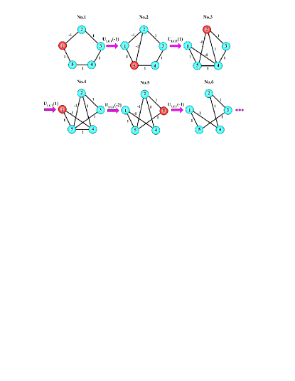
Figure 4: (Color online). Example of the graph rule of the LG operation $U_{LG_{a}}$ repeatedly applied on a CV weighted graph state. The rule is successively applied to the vertex, which is colored with red in the figure.

This LC operation may be applied repeatedly on a CV weighted graph state, which can generate the LC equivalence class of this graph state. Figure 4 shows an example of how to repeatedly apply this rule to obtain the LC equivalence class of a CV weighted graph state. Note that the elements in the LC equivalence class of a CV weighted graph state, generated by the LC operation $U_{LG_{a}}$, are infinite, and whether the whole LC equivalence class of a CV weighted graph state can be obtained by repeatedly applying this LC operation, still need be further investigated.

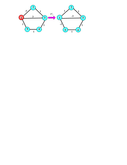
Figure 5: (Color online). Example of the graph rule of the LG operation $F^{2}$ applied on a CV weighted graph state.

At last, the graph rules of two extra and very useful LC operations are presented. One of the LC operations is $F^{2}$, corresponding to the square of the Fourier transform operator, which is used in Ref.seventeen . This operation has the effect of taking $F^{2}\hat{x}(F^{2})^{-1}=-\hat{x}$ and $F^{2}\hat{p}(F^{2})^{-1}=-\hat{p}$. The graph rule of applying this LC operation $F^{2}$ on a vertex a is described as: add the negative sign on the weight factor of all edges connecting the vertex a. An example for the LC operation $F^{2}$ is shown in Fig.5. The other LC operation is $S(r)=exp[ir(\hat{x}\hat{p}+\hat{p}\hat{x})/2]$ with $r\in\mathbb{R}$, which is a quadrature squeezing operation for CV corresponding to the the phase-sensitive optical parametric amplifier. The action of $S(r)$ on the position and momentum operators is $S(r)\hat{x}S(r)^{-1}=\hat{x}e^{r}$ and $S(r)\hat{p}S(r))^{-1}=\hat{p}e^{-r}$, which means to stretch the position component and squeeze the momentum component of an optical field. The graph rule of applying this LC operation $S(r)$ on a vertex a is described as: multiply $e^{-r}$ on the weight factor of all edges connecting the vertex a. An example for the LC operation $S(r)$ is shown in Fig.6. Note that whether these two LC operations are the necessary transformations for the LC equivalence of CV weighted graph states, still need be further studied.

Figure 6: (Color online). Example of the graph rule of the LG operation $S(r)$ applied on a CV weighted graph state.

In summary, the corresponding LC operation of local complementation for qubit graph states is extended to CV weighted graph states. This LC operation may be applied repeatedly on a CV weighted graph state, which can generate the local Clifford equivalence class of this graph state with the infinite elements. This work is an important step to characterize the LC equivalence class of CV weighted graph states. It is natural to raise the question with this work whether a polynomial time algorithm can be found to decide whether two CV graph states are LG equivalent and the action of local Gaussian group on CV graph states can be translated into elementary graph transformations characterized by several simple rules just like qubit graph states. Furthermore, LU equivalence for CV graph states, which is same as that for qubit graph states, also is an open problem.

^†Corresponding author’s email address: jzhang74@sxu.edu.cn, jzhang74@yahoo.com

I ACKNOWLEDGMENTS

J. Zhang thanks K. Peng and C. Xie for the helpful discussions. This research was supported in part by NSFC for Distinguished Young Scholars (Grant No. 10725416), National Basic Research Program of China (Grant No. 2006CB921101), NSFC Project for Excellent Research Team (Grant No. 60821004), NSFC (Grant No. 60678029), Program for the Top Young and Middle-aged Innovative Talents of Higher Learning Institutions of Shanxi and NSF of Shanxi Province (Grant No. 2006011003).

References

- (1) M. Hein, et al., Phys. Rev. A 69, 062311 (2004).
- (2) H. J. Briegel and R. Raussendorf, Phys. Rev. Lett. 86, 910 (2001).
- (3) D. Gottesman, PhD thesis, Caltech, 1997. quant-ph/9705052.
- (4) R. Raussendorf, H. J. Briegel, Phys. Rev. Lett. 86, 5188 (2001).
- (5) S. L. Braunstein and A. K. Pati, Quantum Information with Continuous Variables (Kluwer Academic, Dordrecht, 2003).
- (6) S. L. Braunstein, P. van Loock, Rev. Mod. Phys. 77, 513 (2005).
- (7) J. Zhang, S. L. Braunstein, Phys. Rev. A 73, 032318 (2006).
- (8) P. van Loock, C. Weedbrook and M. Gu, Phys. Rev. A 76, 032321 (2007).
- (9) N. C. Menicucci et al.,Phys. Rev. A 76, 010302 (2007).
- (10) X. Su, et al., Phys. Rev. Lett. 98, 070502 (2007).
- (11) M. Yukawa, et al., Phys. Rev. A 78, 012301 (2008).
- (12) N. C. Menicucci et al., Phys. Rev. Lett. 97, 110501 (2006); P. van Loock, J. Opt. Soc. Am. B 24, 340 (2007).
- (13) J. Zhang, C. Xie, and K. Peng, arXiv:0711.0820[quant-ph].
- (14) M. Hein, et al., quant-ph/0602096.
- (15) M. Van den Nest, J. Dehaene, and B. De Moor, Phys. Rev. A 69, 022316 (2004).
- (16) M. Van den Nest, J. Dehaene, and B. De Moor, Phys. Rev. A 70, 034302 (2004).
- (17) M. Van den Nest, J. Dehaene, and B. De Moor, Phys. Rev. A 71, 062323 (2005); D. Gross, and M. Van den Nest, arXiv:0707.4000[quant-ph]; B. Zeng, H. Chung, A. W. Cross, and I. L. Chuang, Phys. Rev. A 75, 032325 (2007); Z. Ji, J. Chen, Z. Wei, and M. Ying, arXiv:0709.1266[quant-ph].
- (18) J. Zhang, Phys. Rev. A 78, 034301 (2008).
- (19) S. D. Bartlett, et al., Phys. Rev. Lett. 88, 097904 (2002).