Accuracy of the Tracy-Widom limit for the largest eigenvalue in white Wishart matrices

Abstract

Let $A$ be a $p$-variate real Wishart matrix on $n$ degrees of freedom with identity covariance. The distribution of the largest eigenvalue in $A$ has important applications in multivariate statistics. Consider the asymptotics when $p$ grows in proportion to $n$, it is known from Johnstone (2001) that after centering and scaling, these distributions approach the orthogonal Tracy-Widom law for real-valued data, which can be numerically evaluated and tabulated in software.

Under the same assumption, we show that more carefully chosen centering and scaling constants improve the accuracy of the distributional approximation by the Tracy-Widom limit to second order: $\mathrm{O}\left({(n\wedge p)^{-2/3}}\right)$. Together with the numerical simulation, it implies that the Tracy-Widom law is an attractive approximation to the distributions of these largest eigenvalues, which is important for using the asymptotic result in practice. We also provide a parallel accuracy result for the smallest eigenvalue of $A$ when $n>p$.

Key Words and Phrases. Eigenvalues of random matrices, Laguerre orthogonal ensemble, Laguerre polynomial, Liouville-Green method, principal component analysis, rate of convergence, Tracy-Widom distribution, Wishart distribution.

1 Introduction

The central object of multivariate statistical analysis is an $n\times p$ data matrix $X$, where each of the $n$ rows corresponds to an observation of a random vector in a $p$-dimensional space. If we assume that the row vectors are i.i.d. samples from a multivariate Gaussian distribution $N_{p}(\mu,\Sigma)$, much of the classical theory in multivariate statistical analysis is reduced to study of the eigen-decomposition of a random matrix following a Wishart distribution. Typical examples include but are not limited to principal component analysis (PCA), factor analysis and multidimensional scaling (MDS). The fundamental setting is the determinantal equation

$$\det(A-\lambda I)=0\,,$$

where $A$ follows a central Wishart distribution with covariance matrix $\Sigma$.

In this setting, a common null hypothesis is $H_{0}:\Sigma=I$. For instance, in PCA, this is the hypothesis of isotropic variation over all the principal components; see, for example, Mardia et al. (1979, Section 8.4.3). If $H_{0}$ is true, we say that we are in the null case and call $A$ a (real) white Wishart matrix. For testing this particular hypothesis, as for many others in multivariate statistics, there are two different systematic strategies: one is the likelihood ratio test (LRT), which uses all the eigenvalues of $A$; the other is the union intersection test (UIT) initiated by Roy (1953), which utilizes only the largest (or smallest) eigenvalue of $A$ for the current problem.

An inconvenience of using UIT is that the exact evaluation of the marginal distribution of the extreme sample eigenvalues is not simply tractable, even in the null case considered here. Interested readers are referred to Muirhead (1982, Section 9.7) for the expressions of the marginal distributions in terms of hypergeometric function of matrix argument; see, in particular, Corollary 9.7.2 and 9.7.4 there. We remark that recent work of Koev and Edelman (2006) has developed efficient evaluations of hypergeometric functions of matrix argument and made the computation of the exact marginal distributions possible when both $n$ and $p$ are small.

An alternative approach is to approximate these exact finite sample distributions of the extreme eigenvalues by some other well-understood asymptotic distribution. This kind of approximation is ubiquitous in statistics: the normal approximation to the distribution of the Wald and score statistics, the Chi-square approximation to the Pearson statistic in fitting contingency tables, etc. For the problem studied here, Anderson (2003, Chapter 13) provides a complete summary of the established results in the conventional regime of asymptotics:

$$p n\rightarrow\infty$$ is fixed and .

However, many modern data (microarray data, stock prices, weather forecasting, etc.) we are now dealing with typically have the number of features $p$ very large while the number of observations $n$ much smaller than or just comparable to $p$. For these situations, the classical asymptotics is no longer always appropriate and new asymptotic results that could handle this type of data are desirable.

An advance in this direction was made in Johnstone (2001), where the asymptotic regime was switched to

$$p\rightarrow\infty,n=n(p)\rightarrow\infty\text{ and }n/p\rightarrow\gamma\in(0,\infty).$$ (1)

To state his result, let $X$ be an $n\times p$ data matrix with the $n$ rows i.i.d. following $N_{p}(0,I)$. The $p\times p$ matrix $A=X^{\prime}X$ has a standard Wishart distribution: $A\sim W_{p}(I,n).$ We denote the ordered eigenvalues of $A$ by $\lambda_{1}\geq\cdots\geq\lambda_{p}$. Borrowing tools from the field of Random Matrix Theory (RMT), especially those established in Tracy and Widom (1994, 1996, 1998), Johnstone showed that if we define centering and scaling constants as

$$\mu_{p}=\left(\sqrt{n-1}+\sqrt{p}\right)^{2}\,,\quad\sigma_{p}=\left(\sqrt{n-1}+\sqrt{p}\right)\left(\frac{1}{\sqrt{n-1}}+\frac{1}{\sqrt{p}}\right)^{1/3}\,,$$ (2)

then under condition (1),

$$\frac{\lambda_{1}-\mu_{p}}{\sigma_{p}}\,\stackrel{{\scriptstyle\mathcal{D}}}{{\longrightarrow}}\,W_{1}\sim F_{1}\,,$$ (3)

where $F_{1}$ is the orthogonal Tracy-Widom law, which was originally found by Tracy and Widom (1996) as the limiting law of the largest eigenvalue of a $p\times p$ real Gaussian symmetric matrix. We remark that, prior to Johnstone (2001), as a byproduct of his analysis on random growth model, Johansson (2000) established the scaling limit for the largest eigenvalue in complex white Wishart matrix, which turns out to be the unitary Tracy-Widom law $F_{2}$. We’d also like to mention that for the weak limit (3) to hold, El Karoui (2006a) extended the asymptotic regime (1) to include the cases where $n/p\rightarrow 0$ or $\infty$.

This type of asymptotic result, albeit emerging only recently in the statistics literature, has already found its relevance to applications with modern data. For instance, based on the weak limit (3), Patterson et al. (2006) developed a formal test for the presence of population heterogeneity in a biallelic dataset and suggested a systematic way for assigning statistical significance to successive eigenvectors, which in turn has been used to correct population stratification (Price et al., 2006) and to perform genetic matching (Luca et al., 2008) in genome-wide association studies.

From a statistical point of view, to inform the use of any asymptotic result in practice, we need to have an understanding of the accuracy of the approximation to finite distributions by the limit, which usually appears in the form of a rate of convergence result. In the complex domain, El Karoui (2006b) established such a result for Johansson’s theorem with carefully chosen centering and scaling constants. With his choice, the error term in the Tracy-Widom approximation could be controlled at the order $\mathrm{O}\left({(n\wedge p)^{-2/3}}\right)$, as opposed to $\mathrm{O}\left({(n\wedge p)^{-1/3}}\right)$ by using the original centering and scaling constants in Johansson (2000). For an up-to-date survey of higher order accuracy results of this fashion, we refer to Johnstone (2006, Section 3).

In statistics, we are typically more interested in real-valued data. However, for technical reasons, results for complex-valued data are usually easier to derive under the asymptotic regime (1) than in the real case. Recently, in analyzing the parallel problem for the greatest root statistics for pairs of Wishart matrices (Mardia et al., 1979, Definition 3.7.2), Johnstone (2007) figured out a way to connect the central object of study in the real case to that in the complex case. To be more specific, in both real and complex cases, the problem reduces to the study of operator convergence in appropriate metrics by using standard techniques from Random Matrix Theory. The key observation there is that the crucial element of the operator kernel in the real case could be represented in closed form as a rank one perturbation of the complex kernel; see Johnstone (2007, Eq.(50)), which is a consequence of Adler et al. (2000, Proposition 4.2).

Inspired by Johnstone (2007), we investigate in this paper the rate of convergence for the distributions of properly rescaled largest eigenvalues in real white Wishart matrices to the orthogonal Tracy-Widom law. We remark that, instead of using Adler et al. (2000, Proposition 4.2), the central formula (15) for the “complex to real” connnection in our paper is derived from a slightly earlier result given in Widom (1999, Section 4) which is specific to white Wishart matrices. This new approach not only helps to avoid introducing a further nonlinear transformation after rescaling the largest eigenvalues as in Johnstone (2007) but also enables us to make direct use of the analysis done in El Karoui (2006b) for complex white Wishart matrices.

Statement of the theoretical result. It was suggested in Johnstone (2006) that if we modify the centering and scaling constants from (2) to

$$\begin{split}\tilde{\mu}_{np}&=\left(\sqrt{n-\tfrac{1}{2}}+\sqrt{p-\tfrac{1}{2}}\right)^{2},\\ \tilde{\sigma}_{np}&=\left(\sqrt{n-\tfrac{1}{2}}+\sqrt{p-\tfrac{1}{2}}\right)\left(\frac{1}{\sqrt{n-\tfrac{1}{2}}}+\frac{1}{\sqrt{p-\tfrac{1}{2}}}\right)^{1/3},\end{split}$$ (4)

we might obtain second order accuracy in the Tracy-Widom approximation.

Indeed, the main theoretical result of the paper can be formulated as the following theorem, which establishes the above conjecture.

Theorem 1.

Let $A\sim W_{p}(I,n)$ and $\lambda_{1}$ be its largest eigenvalue. Define centering and scaling constants $(\tilde{\mu}_{np},\tilde{\sigma}_{np})$ as in (4), then under condition (1), there exists a continuous and nonincreasing function $C(\cdot)$, such that for all real $s_{0}$, there exists an integer $N_{0}(s_{0},\gamma)$ for which we have that for any $s\geq s_{0}$ and $n\wedge p\geq N_{0}(s_{0},\gamma)$,

$$\bigl{|}P\{\lambda_{1}\leq\tilde{\mu}_{np}+\tilde{\sigma}_{np}s\}-F_{1}(s)\bigr{|}\leq C(s_{0})(n\wedge p)^{-2/3}\exp(-s/2)\,.$$

The theorem provides theoretical support for using the Tracy-Widom law $F_{1}$ as approximate largest eigenvalue distribution in the null case. In addition, the numerical investigation pursued in Section 2.1 shows that the approximation yields reasonable accuracy even when $n$ and $p$ are as small as $2$. Therefore, both theoretical and numerical results provide us with the confidence in using the Tracy-Widom approximation for nearly all finite $n\times p$ distributions, at least under the Wishart assumption.

Remark 1.

In fact, Theorem 1 will be proved only when $p$ is even and $n\neq p$ since our method relies on a determinant formula of de Bruijn (1955) which was only established for $p$ even and the Laguerre polynomials which are essential for building the convergence rate are not well-defined when $n=p$. It would be of interest to have some theoretical support for the $p$ odd and the square cases. However, numerical experiments suggest that the Tracy-Widom approximation works just as well for $p$ odd as for $p$ even and for $n=p$ as for $n\neq p$.

Organization of the paper. In Section 2, we first investigate the numerical quality of the Tracy-Widom approximation for finite $n\times p$ distributions, then review some important statistical settings to which our result is relevant and finally discuss several interesting issues involved in this study, including a parallel result for the smallest eigenvalue. The rest of the paper is dedicated to the proof of Theorem 1, mainly with tools from Random Matrix Theory. In Section 3, we start with the formulation of Theorem 1 in RMT terminology. After that, we derive the central formula (15) in this paper and reduce our problem to the study of operator convergence in some appropriate metric. We sketch our proof of the main result in Section 4 by assembling operator theoretic tools and asymptotic bounds on transformed Laguerre polynomials. Finally, Section 5 gives details of the Laguerre asymptotics required in the proof. Appendix A collects various necessary technical details not spelled out fully in the main text. Appendix B discusses the issues mentioned in Section 2.3 in a more concrete manner.

2 Statistical Implications and Discussion

2.1 Quality of the approximation

An important motivation for the current study is to promote practical use of the Tracy-Widom approximation. For example, one could tabulate the $F_{1}$ table and use it to compute $p$-values. With such motivation, we investigate the quality of the approximation with numerical experiments.

Distributional approximation.

First of all, we study the numerical accuracy of the approximation using our centering and scaling constants (4) and compare it with that of the original proposal (2) in Johnstone (2001), with results summarized in Table 1. We first look at the square cases with $n=p=2$, $5$, $20$ and $100$ and then the cases with the same $p$’s but with the ratio $n/p$ fixed at $4:1$, and finally the cases where $p=5$ and $10$ with $n/p$ raised to as high as $100:1$ and $1000:1$, which, in some sense, fall into the situation $n/p\rightarrow\infty$ as discussed in El Karoui (2006a). Finally, in all these cases, we use $R=40,000$ replications.

In terms of accuracy, from the last three columns of Table 1, the approximation seems reasonable at conventional significance levels of $10\%$, $5\%$ and $1\%$ (corresponding to right-hand tails of the distributions) even when $p$ is as small as $2$ or $5$, and keeps improving as $p$ grows large, regardless of the $n/p$ ratio. When $p$ is large, for instance, in the $100\times 100$ and $400\times 100$ cases, the Tracy-Widom law yields reasonable approximation over the whole range of interest and matches the finite distributions almost exactly on the right-hand tail.

In terms of the comparison with the original centering and scaling constants, we could see from the first block of Table 1 that in the square cases, neither method seems superior to the other. However, when the ratio $n/p$ is changed to $4:1$ or larger (see the second and the third blocks of Table 1), the improvement by using the new constants is substantial. The new constants not only provide better absolute accuracy in most of the cases, but also seem to result in a faster convergence to the limiting distribution $F_{1}$.

Last but not least, the good performance on the right tail and the faster convergence by using the new constants, as reflected in Table 1, support our theoretical bound in Theorem 1.

Percentiles	$-3.8954$	$-3.1804$	$-2.7824$	$-1.9104$	$-1.2686$	$-0.5923$	$0.4501$	$0.9793$	$2.0234$
TW	.01	.05	.10	.30	.50	.70	.90	.95	.99
$2\times 2$	.000	.000	.000	.034	.379	.690	.908	.953	.988
	(.000)	(.000)	(.000)	(.015)	(.345)	(.669)	(.902)	(.950)	(.987)
$5\times 5$	.000	.002	.021	.218	.465	.702	.908	.954	.989
	(.000)	(.002)	(.020)	(.213)	(.460)	(.698)	(.907)	(.953)	(.989)
$20\times 20$	.003	.029	.071	.275	.490	.700	.902	.952	.990
	(.003)	(.029)	(.071)	(.274)	(.489)	(.699)	(.901)	(.952)	(.990)
$100\times 100$	.008	.044	.091	.291	.495	.699	.901	.951	.990
	(.008)	(.043)	(.091)	(.291)	(.495)	(.699)	(.901)	(.951)	(.990)
$8\times 2$	.000	.000	.013	.200	.458	.704	.913	.956	.990
	(.000)	(.004)	(.031)	(.274)	(.534)	(.755)	(.931)	(.966)	(.992)
$20\times 5$	.001	.018	.057	.262	.486	.703	.905	.952	.990
	(.002)	(.028)	(.077)	(.305)	(.533)	(.739)	(.919)	(.960)	(.992)
$80\times 20$	.005	.035	.082	.287	.497	.700	.902	.951	.990
	(.006)	(.043)	(.096)	(.312)	(.524)	(.723)	(.911)	(.956)	(.992)
$400\times 100$	.009	.047	.095	.298	.499	.700	.899	.949	.989
	(.010)	(.052)	(.103)	(.312)	(.514)	(.712)	(.905)	(.952)	(.990)
$500\times 5$	.010	.050	.100	.303	.502	.705	.905	.953	.992
	(.022)	(.084)	(.154)	(.387)	(.589)	(.770)	(.932)	(.968)	(.995)
$5000\times 5$	.012	.056	.108	.311	.511	.711	.910	.957	.993
	(.027)	(.098)	(.169)	(.406)	(.606)	(.783)	(.938)	(.971)	(.995)
$1000\times 10$	.010	.049	.099	.296	.500	.701	.902	.952	.991
	(.017)	(.073)	(.136)	(.363)	(.567)	(.754)	(.925)	(.964)	(.993)
$10000\times 10$	.012	.054	.104	.306	.506	.707	.903	.950	.991
	(.022)	(.084)	(.148)	(.381)	(.579)	(.764)	(.927)	(.964)	(.994)
$2\times\text{SE}$	.001	.002	.003	.005	.005	.005	.003	.002	.001

Table 1: Simulations for finite $n\times p$ vs. Tracy-Widom approximation: accuracy comparison of the new centering and scaling constants (4) with that in Johnstone (2001). For each combination of $n$ and $p$, we show in the first line the estimated cumulative probabilities for $\lambda_{1}$, rescaled using (4); and in the second line with parentheses, rescaled using Johnstone (2001, Eq.(1.3) and (1.4)), both computed from $R=40,000$ repeated draws using the Beta-ensemble sampling technique proposed by Dumitriu and Edelman (2002). The conventional significance levels are highlighted in bold font and the last line gives approximate standard errors based on binomial sampling. The orthogonal Tracy-Widom distribution $F_{1}$ was computed using the method proposed in Edelman and Persson (2002) with percentiles obtained by inverse interpolation.

Approximate percentiles.

Except for computing $p$-values, $F_{1}$ could also be used to compute approximate percentiles of finite $n\times p$ distributions. To measure the accuracy of this approximation, we consider the relative error $r_{\alpha}=\theta^{TW}_{\alpha}/\theta_{\alpha}-1$, where $\theta_{\alpha}$ is the exact $100\alpha$-th percentile of the largest eigenvalue in finite $n\times p$ model and $\theta^{TW}_{\alpha}$ is its counterpart obtained from the Tracy-Widom law.

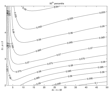
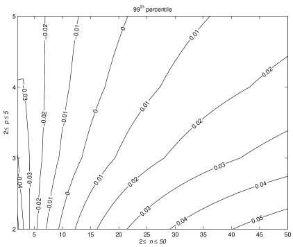
Figure 1: Plots of the relative error $r_{\alpha}=\theta^{TW}_{\alpha}/\theta_{\alpha}-1$ for the approximate percentiles computed from $F_{1}$: (a) $95$-th percentile; (b) $99$-th percentile. The exact finite $n\times p$ largest eigenvalue distributions are computed using Plamen Koev’s implementation in matlab of the recursive method proposed in Koev and Edelman (2006) and the orthogonal Tracy-Widom law $F_{1}$ is computed using the method proposed in Edelman and Persson (2002). The percentiles are always obtained from inverse interpolation.

In Figure 1, we plot the relative error $r_{\alpha}$ for $\alpha=0.95$ and $0.99$, with $p$ ranging from $2$ to $5$ and $n$ from $2$ to $50$. Although the minimum of $n$ and $p$ is no larger than $5$, the numerical accuracy is reasonably satisfactory. For the $95$-th percentile, the relative error ranges from $5\%$ to $10\%$ for most of the cases and slightly exceeds $10\%$ only for the cases where $p=2$ and the $n/p$ ratios are high. The approximation to the $99$-th percentile is even better, with the absolute relative error $\left|r_{.99}\right|\leq 5\%$ for most of the cases. Due to the computational limitation (Koev and Edelman, 2006), we could not compute the exact percentiles when $n$ and $p$ are large. However, we expect the approximate percentiles to become more accurate as the consequence of better distributional approximation.

2.2 Related statistical settings

In this part, we review several common settings in multivariate statistics to which our result is relevant.

Principal component analysis.

Suppose that $X=[{x}_{1},\cdots,{x}_{n}]^{\prime}$ is a Gaussian data matrix. Write the sample covariance matrix ${S}=n^{-1}{X}^{\prime}{H}{X},$ where ${H}={I}-n^{-1}\mathbf{1}\mathbf{1}^{\prime}$ is the centering matrix, principal component analysis looks for a sequence of standardized vectors ${a}_{1},\cdots,{a}_{p}$ in $\mathbb{R}^{p}$, such that for $i=1,\cdots,p$, where ${a}_{i}$ successively solves the following optimization problem:

$$\max\{{a}^{\prime}{S}{a}:\,{a}^{\prime}{a}_{j}=0,\,j\leq i\}\,,$$

where ${a}_{0}$ can be taken as the zero vector. The successive sample principal component eigenvalues $\ell_{1}\geq\cdots\geq\ell_{p}$ then satisfy $\ell_{i}={a}^{\prime}_{i}{S}{a}_{i}$. From a different perspective, these $\ell_{i}$’s may also be found as the roots of the determinantal equation

$$\det({S}-\lambda{I})=0\,.$$

One basic question in the application of PCA is testing the hypothesis of isotropic variation, i.e., the hypothesis that all the population principal component eigenvalues are equal. Under this null hypothesis, the population covariance matrix of the row vectors in ${X}$ is $\sigma^{2}{I}.$ For simplicity, let us suppose that $\sigma^{2}=1$ (if $\sigma^{2}$ is an unknown value, we can estimate it by some $\hat{\sigma}^{2}$ first and divide ${S}$ by $\hat{\sigma}^{2}$). Then the sample covariance matrix ${S}$ satisfies

$$n{S}\sim W_{p}({I},n-1).$$

The largest principal component eigenvalue $\ell_{1}$ of ${S}$ is a natural test statistic for a union intersection test. Our result applies for $n\ell_{1}$.

Multidimensional scaling.

Let ${X}$ be an $n\times p$ data matrix. Consider the centered inner product matrix ${B}={HXX^{\prime}H}$, i.e. ${B}_{ij}=({x}_{i}-\bar{{x}})^{\prime}({x}_{j}-\bar{{x}})$. In a typical setting of multidimensional scaling, we are usually only given the matrix ${B}$ instead of the original observations ${X}$. Let $\lambda_{1}\geq\cdots\geq\lambda_{p}$ be the ordered eigenvalues of ${B}$ and ${v}_{i}$ be the corresponding eigenvector. As defined in Mardia et al. (1979, Section 14.3): for fixed $k$ ($1\leq k\leq p$), the rows of ${V}_{k}=({v}_{1},\cdots,{v}_{k})$ are called the principal coordinates of ${X}$ in $k$ dimensions, which constitute the classical $k$-dimensional solution to the multidimensional scaling problem.

We observe that the matrix ${B}$ shares its non-zero eigenvalues with $n{S}={X^{\prime}HX}$. For the principal coordinate method to make sense, it is important that non-zero eigenvalues of ${B}$ and hence all the eigenvalues of $n{S}$ do not equal a common value. Translated to the population level, the population covariance matrix ${\Sigma}\neq\sigma^{2}{I}.$ Assuming $\sigma^{2}=1$ (or dividing ${B}$ by $\sigma^{2}$ or its estimate $\hat{\sigma}^{2}$), the null hypothesis can be written as $H_{0}:{\Sigma}={I}$. As in the situation of PCA, our result is useful for the test statistic $\ell_{1}$, where $\ell_{1}$ is the largest eigenvalue of ${B}$.

Testing that a covariance matrix equals a specified matrix.

Suppose that we have the Gaussian data matrix $X$ with the rows $x_{1},\cdots,x_{n}$ be independent $N_{p}(\mu,\Sigma)$ random vectors and consider the null hypothesis $H:\Sigma=\Sigma_{0}$, where $\Sigma_{0}$ is a specified positive definite matrix.

If the mean vector $\mathbf{\mu}$ is unknown, let ${S}=n^{-1}{X}^{\prime}{H}{X}$ be the sample covariance matrix. The union intersection test uses the largest eigenvalue of the matrix ${\Sigma}_{0}^{-1}{S}$, denoted by $\lambda_{1}({\Sigma}_{0}^{-1}{S})$, as the test statistic (see Mardia et al., 1979, p.130).

We observe that $\lambda_{1}({\Sigma}_{0}^{-1}{S})=\lambda_{1}({\Sigma}_{0}^{-1/2}{S}{\Sigma}_{0}^{-1/2})$, where under the null hypothesis,

$$n{\Sigma}_{0}^{-1/2}{S}{\Sigma}_{0}^{-1/2}\sim W_{p}({I},n-1).$$

Hence, our result is available for $n\lambda_{1}({\Sigma}_{0}^{-1}{S})$.

Singular value decomposition.

For $X$ a real $n\times p$ matrix, there exists orthogonal matrices $U(n\times n)$ and $V(p\times p)$, such that

$$X=UDV^{T},$$

where $D=\text{diag}(\sigma_{1},\cdots,\sigma_{\min(n,p)})\in\mathbb{R}^{n\times p}$, and $\sigma_{1}\geq\cdots\geq\sigma_{\min(n,p)}\geq 0$. This representation is called the singular value decomposition of $X$ [See Golub and van Loan (1996, Theorem 2.5.2)]. For $1\leq i\leq\min(n,p)$, $\sigma_{i}$ is called the $i$-th singular value of $X$. Theorem 1 then provides an accurate distributional approximation for $\sigma_{1}^{2}$ when the entries of $X$ are independent standard normal.

2.3 Other issues

For here, we provide brief remarks on several interesting issues that we come across during the development of this work. More details about them could be found in Appendix B.

Transformation.

In the analysis of the greatest root statistic, Johnstone (2007) suggested that a nonlinear transformation [the logit transformation: $\tau(x)=\log[x/(1-x)]$ in his case] helps improve the distributional approximation by the Tracy-Widom law, see Theorem 1, Table 1 and Fig. 1 there. In addition to its numerical effect, the transformation has an geometric explanation and yields a very natural integral representation for the correlation kernel which later appears in the central formula Eq.(50) there; see Johnstone (2007, Section 2.2, also Eq.’s (16) and (46)), Forrester (2004, Proposition 4.11) and Adler et al. (2000, Proposition 4.2).

Following Forrester (2004, Proposition 4.11), if we wanted to employ a comparable transformation for our white Wishart case, it would be the logarithmic transformation: $\tau(x)=\log x$. In fact, in our study, we first looked into some depth along this direction and could conclude the following second order accuracy result: under the condition of Theorem 1, let $\nu_{np}=\log{\tilde{\mu}_{np}}$ and $\tau_{np}=\tilde{\sigma}_{np}/\tilde{\mu}_{np}$, there exists a continuous and nonincreasing function $C(\cdot)$, such that for all real $s_{0}$, there exists an integer $N_{0}(s_{0},\gamma)$ for which we have that for any $s\geq s_{0}$ and $n\wedge p\geq N_{0}(s_{0},\gamma)$,

$$\bigl{|}P\{\log\lambda_{1}\leq\nu_{np}+\tau_{np}s\}-F_{1}(s)\bigr{|}\leq C(s_{0})(n\wedge p)^{-2/3}\exp(-s/2)\,.$$ (5)

Some comments on how this result could be derived are included in B.1.

Although the rates of convergence are the same, numerical experiments suggest that using the nonlinear transformation does not yield as good numerical results in distributional approximation for small to moderate $n$ and $p$ as simply rescaling $\lambda_{1}$ using (4), especially on the right-hand tail which is of the most statistical interest. When $n$ and $p$ grow large, using the transformation or not does not have as much influence, as they approach the same limit.

In consideration of the actual quality of approximation, especially for small to moderate $n$ and $p$, we suggest not using the logarithmic transformation for the largest eigenvalues. However, it is of theoretical interest to know why such natural transformation works for the greatest root statistic in Johnstone (2007) but not for the largest eigenvalue in white Wishart matrices here.

The smallest eigenvalue.

Following the principle of union intersection tests, the smallest eigenvalue could also serve as the test statistic in some cases, see, for instance, Mardia et al. (1979, Section 5.2.2c). Hence, what we have established for the largest eigenvalue is also worth investigation for the smallest one. Moreover, understanding the deviation of the smallest eigenvalue from its almost sure limit is also of independent interest. For example, it plays an important role in the theory of sparse signal recovery from large underdetermined linear system. See, for example, Donoho (2004) and Candes and Tao (2006). In fact, as we studied the accuracy result for the largest eigenvalue using the logarithmic transformation, we obtained a parallel result for smallest eigenvalues as a pleasant byproduct. We state without proof the result here.

Suppose that $n-1\geq p$ and $n/p\rightarrow\gamma\in(1,\infty)$ and introduce the reflect Tracy-Widom law (Paul, 2006) as

$$G_{1}(s)=1-F_{1}(-s).$$

Let

$$\mu_{np}^{-}=\left(\sqrt{n-\tfrac{1}{2}}-\sqrt{p-\tfrac{1}{2}}\right)^{2},\sigma_{np}^{-}=\left(\sqrt{n-\tfrac{1}{2}}-\sqrt{p-\tfrac{1}{2}}\right)\left(\frac{1}{\sqrt{p-\tfrac{1}{2}}}-\frac{1}{\sqrt{n-\tfrac{1}{2}}}\right)^{1/3},$$

and then define

$$\tau^{-}_{np}=\sigma^{-}_{np}/\mu^{-}_{np},\quad\text{and}\quad\nu^{-}_{np}=\log\mu^{-}_{np}+\frac{1}{8}\left(\tau^{-}_{np}\right)^{2}.$$ (6)

We then have that for the smallest eigenvalue $\lambda_{p}$ of a $p\times p$ white Wishart matrix with $n$ degrees of freedom, there exists a continuous and nondecreasing function $C(\cdot)$, such that for all real $s_{0}$, there exists an integer $N_{0}(s_{0},\gamma)$ for which we have that for any $s\leq s_{0}$ and $p\geq N_{0}(s_{0},\gamma)$,

$$\bigl{|}P\{\log\lambda_{p}\leq\nu^{-}_{np}+\tau^{-}_{np}s\}-G_{1}(s)\bigr{|}\leq C(s_{0})p^{-2/3}\exp(s/2)\,.$$ (7)

See B.2 for remarks on how to prove this result.

Unlike the case for $\lambda_{1}$, the logarithmic transformation improves the numerical accuracy of the distributional approximation for $\lambda_{p}$ significantly, especially when $p$ is small and $n/p$ is close to $1$. We feel that an intuitive explanation to this phenomenon could be the following: for $\lambda_{p}$, the lower bound at $0$ strongly affects the approximation on the original scale, especially when both $p$ and $n/p$ are small. However, by transforming $\lambda_{p}$ to $\log\lambda_{p}$, one maps the lower bound to $-\infty$ and hence avoids this ‘hard edge’ effect. The largest eigenvalue does not enjoy such a benefit for it does not have an algebraic upper bound.

As a numerical illustration, in Table 2, we present some simulation results on the Tracy-Widom approximation to smallest eigenvalues transformed as above for two $n/p$ ratios: $2:1$ and $4:1$, both with $p=5$, $10$ and $100$. Again, for each combination of $n$ and $p$, we run $R=40,000$ replications. The approximation seems good on the left-hand tail (where traditional significance levels locate) even for $p$ as small as $5$, regardless of the $n/p$ ratio. Moreover, for both $n/p$ ratios, when $p$ grows to $100$, the approximation becomes reasonably accurate over the entire range under investigation and is almost perfect on the left-hand tail. Therefore, the numerical results agree well with the theory for the smallest eigenvalues, too.

Percentiles	3.8954	3.1804	2.7824	1.9104	1.2686	0.5923	-0.4501	-0.9793	-2.0234
RTW	.99	.95	.90	.70	.50	.30	.10	.05	.01
$10\times 5$	1.000	.995	.976	.796	.553	.306	.093	.045	.012
$20\times 10$	.999	.984	.952	.760	.536	.305	.098	.049	.011
$200\times 100$	.993	.958	.910	.708	.504	.301	.099	.050	.010
$20\times 5$	.998	.977	.939	.745	.527	.306	.097	.049	.010
$40\times 10$	.996	.969	.926	.726	.511	.300	.098	.048	.010
$400\times 100$	.993	.955	.905	.703	.501	.301	.100	.050	.010
$2\times\text{SE}$	.001	.002	.003	.005	.005	.005	.003	.002	.001

Table 2: Simulations for finite $n\times p$ vs. Tracy-Widom approximation: the smallest eigenvalue. For each combination of $n$ and $p$, the estimated cumulative probabilities are computed for $(\log\lambda_{p}-\nu^{-}_{np})/\tau^{-}_{np}$ with $R=40,000$ draws from $W_{p}(I,n)$. The methods of sampling, computing $F_{1}$ and obtaining percentiles are the same as in Table 1. The conventional significance levels are highlighted in bold font and the last line gives approximate standard errors based on binomial sampling.

3 Random Matrix Theory

The establishment of Theorem 1 relies heavily on results and methods from Random Matrix Theory (RMT) literature. In particular, those about unitary and orthogonal Laguerre matrix ensembles play an important role. In this section, we first restate our main result using RMT terminology. With a Lipschitz-type bound, we transform the problem into the study of convergence rate of operators with matrix kernels and derive the closed form representation (15) of the top-left entry in the kernel for Laguerre orthogonal ensemble. Finally, we study the effect of scaling on our kernel representation and carefully formulate the analysis problem to be solved in later sections.

3.1 Restatement of Theorem 1 in Random Matrix Theory

Suppose $A$ is an $N\times N$ matrix following a $W_{N}(I,n)$ distribution with $n>N$. [Here and after, following the RMT notational convention, we use $N$ rather than $p$ to denote the number of features.] The celebrated joint probability density function of the eigenvalues $x_{1}\geq\cdots\geq x_{N}\geq 0$ is given by (Muirhead, 1982):

$$p_{N}(x_{1},\cdots,x_{N})=d_{n,N}^{-1}\prod_{1\leq j<k\leq N}(x_{j}-x_{k})\prod_{j=1}^{N}x_{j}^{n-N-1}e^{-x_{j}/2},$$

where $d_{n,N}$ is a normalizing constant depending only on $n$ and $N$.

On the other hand, RMT people have investigated Laguerre Orthogonal Ensembles (LOE), where ‘ensemble’ stands for distribution of matrices and ‘orthogonal’ refers to the invariance of the distribution under orthogonal transformations. The LOE($N,\tilde{\alpha}$) model ($\tilde{\alpha}>-1$) has the matrix eigenvalue density as

$$\tilde{p}_{N}(x_{1},\cdots,x_{N})=d^{-1}_{\tilde{\alpha},N}\prod_{1\leq j<k\leq N}(x_{j}-x_{k})\prod_{j=1}^{N}x_{j}^{\tilde{\alpha}}e^{-x_{j}/2},$$ (8)

where $x_{1}\geq\cdots\geq x_{N}\geq 0$ and $d_{\tilde{\alpha},N}$ is a normalizing constant depending only on $N$ and $\tilde{\alpha}$.

If we define $\alpha_{N}=n-N$, the joint eigenvalue density of white Wishart matrix $A$ is exactly the eigenvalue density of the LOE($N,\alpha_{N}-1$) model. By this observation, we can formulate Theorem 1 in terms of RMT as the following.

Theorem 2.

Let $x_{1}$ be the largest eigenvalue in the LOE($N,\alpha_{N}-1$) model and $F_{1}$ be the orthogonal Tracy-Widom law. Define $\tilde{\mu}_{n,N}$ and $\tilde{\sigma}_{n,N}$ as

$$\tilde{\mu}_{n,N}=\left(\sqrt{n-\tfrac{1}{2}}+\sqrt{N-\tfrac{1}{2}}\right)^{2},\,\tilde{\sigma}_{n,N}=\left(\sqrt{n-\tfrac{1}{2}}+\sqrt{N-\tfrac{1}{2}}\right)\left(\frac{1}{\sqrt{n-\tfrac{1}{2}}}+\frac{1}{\sqrt{N-\tfrac{1}{2}}}\right)^{1/3}.$$ (9)

If $n>N$, $N\rightarrow\infty,n=n(N)\rightarrow\infty$ and $n/N\rightarrow\gamma\in[1,\infty)$, there exists a continuous and nonincreasing function $C(\cdot)$, such that for all real $s_{0}$, there exists an integer $N_{0}(s_{0},\gamma)$ for which we have that for any $s\geq s_{0}$ and $N\geq N_{0}(s_{0},\gamma)$,

$$\bigl{|}P\{x_{1}\leq\tilde{\mu}_{n,N}+\tilde{\sigma}_{n,N}s\}-F_{1}(s)\bigr{|}\leq C(s_{0})N^{-2/3}\exp(-s/2)\,.$$

Remark 2.

The theorem is stated only for situations where $n>N$. It works equally well when $n<N$ by switching $n$ and $N$. This results from the following observations: (a) constants in (9) are symmetric in $n$ and $N$ and (b) switching $n$ and $N$ does not change the distribution of $x_{1}$.

3.2 Operator determinant and kernel representation

We focus on the LOE($N,\tilde{\alpha}$) model in (8) for the moment. For general orthogonal ensembles, Tracy and Widom (1998, Section 9) showed that when $N$ is even, for $\chi=I_{x>x^{\prime}}$:

$$F_{N,1}(x^{\prime})\equiv P\{x_{1}\leq x^{\prime}\}=\sqrt{\det(I-K_{N}\chi)},$$ (10)

with $K_{N}$ an operator with a $2\times 2$ matrix kernel:

$$K_{N}(x,y)=\begin{pmatrix}I&-\partial_{2}\\ \varepsilon_{1}&T\end{pmatrix}S_{N,1}(x,y)-\begin{pmatrix}0&0\\ \varepsilon(x-y)&0\end{pmatrix}\ ,$$ (11)

where $\partial_{2}$ is the differential operator with respect to the second argument, $\varepsilon_{1}$ is the convolution operator acting on the first argument with the kernel $\varepsilon(x-y)=\frac{1}{2}\text{sgn}(x-y)$ and $TS(x,y)=S(y,x)$ for any kernel $S$. However, no explicit representation of $S_{N,1}$ was given there.

In a follow-up paper, Widom (1999) derived explicit expression of the kernel $S_{N,1}$ for Gaussian and Laguerre orthogonal ensembles, which is summarized in Adler et al. (2000, Eq.(4.3)) in a more friendly form. In particular, for the LOE($N,\tilde{\alpha}$) model of our interest, we have [Warning: we need to switch $x$ and $y$ in Adler et al. (2000, Eq.(4.3)).]:

$$\begin{split}S_{N,1}(x,y)=S_{N,2}(x,y)+&\frac{N!}{4\Gamma(N+\tilde{\alpha})}x^{\tilde{\alpha}/2}e^{-x/2}\left(\frac{d}{dx}L_{N}^{\tilde{\alpha}}(x)\right)\\ &\times\int_{0}^{\infty}\text{sgn}(y-z)z^{\tilde{\alpha}/2-1}e^{-z/2}[L_{N}^{\tilde{\alpha}}(z)-L_{N-1}^{\tilde{\alpha}}(z)]dz,\end{split}$$ (12)

where $L_{k}^{\tilde{\alpha}}$ $(k=N-1,N)$ are Laguerre polynomials defined in Szegö (1975, Chapter V) and $S_{N,2}(x,y)$ is the kernel related to the Laguerre unitary ensemble (LUE) with parameter ($N,\tilde{\alpha}$), which has the following eigenvalue density:

$$p_{N}(x_{1},\cdots,x_{N})=c_{n,N}^{-1}\prod_{1\leq j<k\leq N}(x_{j}-x_{k})^{2}\prod_{j=1}^{N}x_{j}^{\tilde{\alpha}}e^{-x_{j}},\quad x_{1}\geq\cdots\geq x_{N}\geq 0.$$

With (12), we start to derive an closed form representation for $S_{N,1}$ after some necessary definitions. As in Johnstone (2001), we define a basis $\{\phi_{k}\}_{k=0}^{\infty}$ on $L^{2}([0,\infty))$ with transformed Laguerre polynomials

$$\phi_{k}(x;\tilde{\alpha})=\sqrt{\frac{k!}{(k+\tilde{\alpha})!}}\,x^{\tilde{\alpha}/2}e^{-x/2}L_{k}^{\tilde{\alpha}}(x).$$ (13)

Then calling $a_{N}=\sqrt{N(N+\tilde{\alpha})}$, we follow El Karoui (2006b, Section 2) to introduce for $x\geq 0$,

$$\phi(x;\tilde{\alpha})=(-1)^{N}\sqrt{\frac{a_{N}}{2}}\phi_{N}(x;\tilde{\alpha}-1)x^{-1/2};\quad\psi(x;\tilde{\alpha})=(-1)^{N-1}\sqrt{\frac{a_{N}}{2}}\phi_{N-1}(x;\tilde{\alpha}+1)x^{-1/2}.$$ (14)

With the definition in (14), for the first term in (12), Johnstone (2001, Eq.(3.6)) and El Karoui (2006b, Appendix A.5) gave the following integral representation

$$S_{N,2}(x,y)=\int_{0}^{\infty}\phi(x+z)\psi(y+z)+\psi(x+z)\phi(y+z)dz.$$

For the second term, we could apply Szegö (1975, Eq.(5.1.13), (5.1.14)) to obtain that it equals

$$-\frac{N!}{4\Gamma(N+\tilde{\alpha})}x^{\tilde{\alpha}/2}e^{-x/2}L_{N-1}^{\tilde{\alpha}+1}(x)\int_{0}^{\infty}\text{sgn}(y-z)z^{\tilde{\alpha}/2-1}e^{-z/2}L_{N}^{\tilde{\alpha}-1}(z)dz=\psi(x)\int_{0}^{\infty}\varepsilon(y-z)\phi(z)dz.$$

Hence, we obtain

$$S_{N,1}(x,y)=S_{N,2}(x,y)+\psi(x)\int_{0}^{\infty}\varepsilon(y-z)\phi(z)dz.$$

Recall that for the white Wishart matrix $A\sim W_{N}(I,n)$, setting $\alpha_{N}=n-N$, it is connected to the LOE($N,\tilde{\alpha}$) model by the identity $\tilde{\alpha}=\alpha_{N}-1$. Thus, if we use the parameters $N$ and $\alpha_{N}$, then the above calculation gives the following representation for $S_{N,1}$:

$$\boxed{S_{N,1}(x,y;\alpha_{N}-1)=S_{N,2}(x,y;\alpha_{N}-1)+\psi(x;\alpha_{N}-1)\int_{0}^{\infty}\varepsilon(y-z)\phi(z;\alpha_{N}-1)dz.}$$ (15)

3.2.1 Framework for deriving the determinant formula

The determinant formula (10) introduced at the beginning of this subsection provides the foundation for the convergence arguments. However, it is worth clarification under which framework it is derived.

Tracy and Widom (2005) described with care the operator convergence of $K_{N}\chi$ to the limit $K_{GOE}$ for the Hermite finite $N$ ensemble. We adapt and extend their approach to the Laguerre finite $N$ ensemble. Therefore, we paraphrase their remarks on the weighted Hilbert spaces and regularized $2$-determinants under the current setting.

In the kernel $K_{N}$ given in (11), the first term on the right hand side has each of its entries finite rank operators and hence a trace class operator. However, this is not true for $\varepsilon(x-y)$. According to Reed and Simon (1980, Theorem VI.23), it is even not Hilbert-Schmidt on $L^{2}([x^{\prime},\infty))$. One way to take care of this problem is to introduce the weighted $L^{2}$ space and to generalize the operator determinant as in Tracy and Widom (2005).

To this end, let $\rho$ be any weight function which satisfies the following two conditions:

1. its reciprocal $\rho^{-1}\in L^{1}([0,\infty))$; and

2. each operator that constitutes elements in the first term on the right hand side of (11) is in $L^{2}([x^{\prime},\infty);\rho)\cap L^{2}([x^{\prime},\infty);\rho^{-1})$.

Then, as remarked in Tracy and Widom (2005), $\varepsilon$: $L^{2}([x^{\prime},\infty);\rho)\rightarrow L^{2}([x^{\prime},\infty);\rho^{-1})$ is Hilbert-Schmidt. Moreover, $K_{N}$ could now be regarded as a $2\times 2$ matrix kernel on the space $L^{2}([x^{\prime},\infty);\rho)\oplus L^{2}([x^{\prime},\infty);\rho^{-1})$.

We have thus made clear on which space the kernel $K_{N}$ acts. In order for the determinant formula (10) to hold, we need a generalization of the usual Fredholm determinant for trace class operators to determinant for Hilbert-Schmidt operators.

By our condition on $\rho$, for $K_{N}=[K_{ij}]_{1\leq i,j\leq 2}$, we regard $K_{11}$ and $K_{22}$ as trace class operators on $L^{2}([x^{\prime},\infty);\rho)$ and $L^{2}([x^{\prime},\infty);\rho^{-1})$ respectively and off-diagonal elements as Hilbert-Schmidt operators:

$$K_{12}:L^{2}([x^{\prime},\infty);\rho^{-1})\rightarrow L^{2}([x^{\prime},\infty);\rho)\quad\text{and}\quad K_{21}:L^{2}([x^{\prime},\infty);\rho)\rightarrow L^{2}([x^{\prime},\infty);\rho^{-1}).$$

Hence, $\text{tr}(K_{N})=\text{tr}(K_{11})+\text{tr}(K_{22})$ is well defined. The regularized 2-determinant of Hilbert-Schmidt operator $T$ with eigenvalues $\mu_{k}$ is defined by

$${\det}_{2}(I-T)=\prod_{k}(1-\mu_{k})e^{\mu_{k}}.$$

Then one naturally extends the operator definition of determinants to Hilbert-Schmidt operator matrix $T$ with trace class diagonal entries by setting

$$\det(I-T)={\det}_{2}(I-T)\exp(-\text{tr}T).$$ (16)

Finally, as remarked in Tracy and Widom (2005), the resulting notion of $\det(I-K_{N})$ is independent of the choice of $\rho$ and allows the derivation in Tracy and Widom (1998) that yields (10), (11) and eventually (15).

Later in Section 4.1.1, we will make a specific choice of $\rho$, which not only makes our arguments more explicit but also eases the derivation of the right tail exponential decay in our desired bound.

3.3 Scaling the kernel

Fixing any real number $s_{0}$ and introducing the linear transformation $\tau(s)=\tilde{\mu}_{n,N}+{s}\tilde{\sigma}_{n,N}$, we are interested in the convergence rate of $F_{N,1}(\tau(s^{\prime}))$ to $F_{1}(s^{\prime})$ for all $s^{\prime}\geq s_{0}$.

Define the rescaled kernel $K_{\tau}$ as the following:

$$K_{\tau}(s,t)=\sqrt{\tau^{\prime}(s)\tau^{\prime}(t)}\,K_{N}(\tau(s),\tau(t))=\tilde{\sigma}_{n,N}K_{N}(\tilde{\mu}_{n,N}+{s}\tilde{\sigma}_{n,N},\tilde{\mu}_{n,N}+{t}\tilde{\sigma}_{n,N}).$$

We have $\det(I-K_{N})=\det(I-K_{\tau})$ by noticing that $K_{N}$ and $K_{\tau}$ share the spectrum. We give below an explicit representation of $K_{\tau}$ for later use.

Before we proceed, we apply the $\tau$-scaling to $\phi$, $\psi$ and $S_{N,2}$ and thus define

$$\phi_{\tau}(s)=\tilde{\sigma}_{n,N}\phi(\tilde{\mu}_{n,N}+{s}\tilde{\sigma}_{n,N}),\quad\psi_{\tau}(s)=\tilde{\sigma}_{n,N}\psi(\tilde{\mu}_{n,N}+{s}\tilde{\sigma}_{n,N})$$ (17)

and

$$\begin{split}S_{\tau}(s,t)&=\tilde{\sigma}_{n,N}S_{N,2}(\tilde{\mu}_{n,N}+{s}\tilde{\sigma}_{n,N},\tilde{\mu}_{n,N}+{t}\tilde{\sigma}_{n,N})\\ &=\int_{0}^{\infty}\phi_{\tau}(s+z)\psi_{\tau}(t+z)+\psi_{\tau}(s+z)\phi_{\tau}(t+z)dz.\end{split}$$ (18)

For later convenience, $\phi_{\tau}(s)$ and $\psi_{\tau}(s)$ are assumed to be $0$ when $\tau(s)=\tilde{\mu}_{n,N}+{s}\tilde{\sigma}_{n,N}<0$, and hence they are well-defined on the entire real line.

Finally, we introduce the short notation

$$S_{\tau}^{R}(s,t)=S_{\tau}(s,t)+\psi_{\tau}(s)\int_{-\infty}^{\infty}\varepsilon(t-z)\phi_{\tau}(z)dz=S_{\tau}(s,t)+\psi_{\tau}(s)\left(\varepsilon\phi_{\tau}\right)(t).$$ (19)

[We remind the reader that in the above discussion, we have dropped the explicit dependence on $\tilde{\alpha}$ or $\alpha_{N}-1$ to avoid notation nightmare. Henceforth, we mention the explicit dependence only for eliminating ambiguity.]

We further observe that the determinant formula does not change if we modify $K_{\tau}$ as

$$K_{\tau}(s,t)=\begin{pmatrix}K_{\tau,11}(s,t)&\tilde{\sigma}_{n,N}K_{\tau,12}(s,t)\\ \tilde{\sigma}_{n,N}^{-1}K_{\tau,21}(s,t)&K_{\tau,22}(s,t)\end{pmatrix}\ ,$$

for the spectrum does not change. Based on this observation and our detailed calculation in A.2, we could represent the entries of $K_{\tau}$ as

$$\begin{split}K_{\tau,11}(s,t)=S^{R}_{\tau}(s,t),\qquad&K_{\tau.12}(s,t)=-\partial_{t}S^{R}_{\tau}(s,t),\\ K_{\tau,21}(s,t)=(\varepsilon_{1}S^{R}_{\tau})(s,t)-\varepsilon(s-t),\qquad&K_{\tau,22}(s,t)=K_{\tau,11}(t,s).\end{split}$$ (20)

For the desired limit $F_{1}(s^{\prime})$ of the sequence $F_{N,1}(s^{\prime})$, Tracy and Widom (2005) showed that $F_{1}(s^{\prime})=\sqrt{\det(I-K_{GOE})}$, where the operator $K_{GOE}$ has the matrix kernel

$$K_{GOE}(s,t)=\begin{pmatrix}S(s,t)&SD(s,t)\\ IS(s,t)-\varepsilon(s-t)&S(t,s)\end{pmatrix}$$

with the entries given by

$$\begin{split}S(s,t)=S_{A}(s,t)+\frac{1}{2}\text{Ai}(s)\left(1-\int_{t}^{\infty}\text{Ai}(u)du\right),\quad SD(s,t)=-\partial_{t}S_{A}(s,t)-\frac{1}{2}\text{Ai}(s)\text{Ai}(t)\\ \text{and}\quad IS(s,t)=-\int_{s}^{\infty}S_{A}(u,t)du+\frac{1}{2}\left(\int_{t}^{s}\text{Ai}(u)du+\int_{s}^{\infty}\text{Ai}(u)du\int_{t}^{\infty}\text{Ai}(u)du\right).\end{split}$$

Here $S_{A}(s,t)=\int_{0}^{\infty}\text{Ai}(s+u)\text{Ai}(t+u)du$ represents the Airy kernel with $\text{Ai}(\cdot)$ the Airy function defined in Olver (1974, p.53, Eq.(8.01)).

By our discussion in Section 3.2.1, it is necessary that both $K_{\tau}$ and $K_{GOE}$ belong to the following class $\mathcal{A}$ of operators

$$\begin{split}\mathcal{A}\equiv\{&\text{$2\times 2$ Hilbert-Schmidt operator matrices $A$ on}\\ &\quad\text{$L^{2}([s^{\prime},\infty);\rho\circ\tau)\oplus L^{2}([s^{\prime},\infty);\rho^{-1}\circ\tau)$ with trace class diagonal entries}\}.\end{split}$$ (21)

This fact will be verified after we choose a specific $\rho$ in Section 4.1.1. For the convenience of argument, let us assume it for the moment.

3.4 Lipschitz bound and kernel difference

Let $p_{N}=F_{N,1}(s^{\prime})$ and $p_{\infty}=F_{1}(s^{\prime})$, we note that $|p_{N}-p_{\infty}|\leq|p_{N}^{2}-p_{\infty}^{2}|/p_{\infty}\leq C(s_{0})|p_{N}^{2}-p_{\infty}^{2}|$, where $C(s_{0})=1/F_{1}(s_{0})$ which is continuous and non-increasing in $s_{0}$. Thus, we are led to the difference of the determinants

$$\left|F_{N,1}(s^{\prime})-F_{1}(s^{\prime})\right|\leq C(s_{0})\left|\det(I-K_{\tau})-\det(I-K_{GOE})\right|.$$ (22)

Remark 3.

Here and after, we use $C(s_{0})$ to denote in general any continuous and non-increasing function of $s_{0}$ and $C$ any universal constant, where the actual function and constant might be different from display to display.

To study the quantity on the right hand side of (22), our basic tool is the following Lipschitz-type bound on the matrix operator determinant for operators in $\mathcal{A}$.

Proposition 1.

For operators $A$ and $B$ in class $\mathcal{A}$ and determinants of $I-A$ and $I-B$ defined as in (16), if $\sum_{i}\|A_{ii}-B_{ii}\|_{1}+\sum_{i\neq j}\|A_{ij}-B_{ij}\|_{2}\leq 1/2$, then

$$\left|\det(I-A)-\det(I-B)\right|\leq M(B)\left(\sum_{i}\|A_{ii}-B_{ii}\|_{1}+\sum_{i\neq j}\|A_{ij}-B_{ij}\|_{2}\right),$$ (23)

where $M(B)=2\,\left|\det(I-B)\right|+2\exp\left[2\left(1+\|B\|_{2}\right)^{2}+\sum_{i}\|B_{ii}\|_{1}\right].$

Note that the leading term on the right hand side of (23) depends only on $B$. In this sense, Proposition 1 is a refinement of Proposition 3 in Johnstone (2007). Its proof could be found in A.5.

By Proposition 1, if we could control the entry-wise convergence rate of $K_{\tau}$ to $K_{GOE}$, we will be able to bound the right hand side of (22) and hence prove our theorem. To this end, a convenient expression of the kernel difference $K_{\tau}-K_{GOE}$ is helpful. we derive such an expression below by essentially adapting the arguments in Johnstone (2007, Section 8.3) to the current context.

According to Nagao and Forrester (1995, Eq.(4.2)), we could calculate [see A.1 for detail] that when $N$ is even,

$$\begin{split}\int_{-\infty}^{\infty}\psi_{\tau}(s;\alpha_{N}-1)ds&=0,\quad\text{and}\\ \int_{-\infty}^{\infty}\phi_{\tau}(s;\alpha_{N}-1)ds&=\frac{N^{1/4}(n-1)^{1/4}}{2^{(\alpha_{N}-3)/2}(N+1)}\frac{\Gamma\left(\frac{N+3}{2}\right)}{\Gamma\left(\frac{n+1}{2}\right)}\left[\frac{\Gamma(n)}{\Gamma(N+1)}\right]^{1/2}.\end{split}$$

For later use, we define $\beta_{N}=\frac{1}{2}\int_{-\infty}^{\infty}\phi_{\tau}(s)ds$.

Bring in the right-tail integration operator $\tilde{\varepsilon}$ introduced in Johnstone (2007, Section 8.3) as

$$(\tilde{\varepsilon}{g})(s)\equiv\int_{s}^{\infty}g(u)du,$$ (24)

we have the identity $(\varepsilon{g})(s)=\frac{1}{2}\int_{-\infty}^{\infty}g(u)du-(\tilde{\varepsilon}{g})(s)$ and hence obtain

$$\varepsilon\phi_{\tau}=\beta_{N}-\tilde{\varepsilon}\phi_{\tau},\quad\text{and}\quad\varepsilon\psi_{\tau}=-\tilde{\varepsilon}\psi_{\tau}.$$

For $S_{\tau}$ defined in (18), by Fubini’s theorem [justified by Lemma 1]

$$\int_{-\infty}^{\infty}S_{\tau}(u,t)du=2\beta_{N}\int_{0}^{\infty}\psi_{\tau}(t+z)dz=2\beta_{N}(\tilde{\varepsilon}\psi_{\tau})(t).$$

Observing that for any kernel $A(s,t)$, $(\varepsilon_{1}A)(s,t)=\frac{1}{2}\int_{-\infty}^{\infty}A(u,t)du-\int_{s}^{\infty}A(u,t)du$, and introducing the abbreviation $a\otimes b$ for rank one operator with kernel $a(s)b(t)$, we have $\varepsilon_{1}S_{\tau}=\beta_{N}\otimes\tilde{\varepsilon}\psi_{\tau}-\tilde{\varepsilon}_{1}S_{\tau}$, and for $S_{\tau}^{R}$ in (19), we have $S^{R}_{\tau}=S_{\tau}+\psi_{\tau}\otimes\beta_{N}-\psi_{\tau}\otimes\tilde{\varepsilon}\phi_{\tau},$ which finally gives

$$\varepsilon_{1}S^{R}_{\tau}=-\tilde{\varepsilon}_{1}\left(S_{\tau}-\psi_{\tau}\otimes\tilde{\varepsilon}\phi_{\tau}\right)+\beta_{N}\left(1\otimes\tilde{\varepsilon}\psi_{\tau}-\tilde{\varepsilon}\psi_{\tau}\otimes 1\right).$$

By the explicit expressions for $K_{\tau}$ entries in (20),

$$K_{\tau}(s,t)=\begin{pmatrix}S^{R}_{\tau}(s,t)&-\partial_{t}S^{R}_{\tau}(s,t)\\ \varepsilon_{1}S^{R}_{\tau}(s,t)&S^{R}_{\tau}(t,s)\end{pmatrix}+\begin{pmatrix}0&0\\ -\varepsilon(s-t)&0\end{pmatrix}=LS^{R}_{\tau}+K^{\varepsilon},$$

where

$$L=\begin{pmatrix}I&-\partial_{2}\\ \varepsilon_{1}&T\end{pmatrix}\quad\text{and}\quad K^{\varepsilon}=\begin{pmatrix}0&0\\ -\varepsilon&0\end{pmatrix}.$$

We then decompose $K_{\tau}$ and $K_{GOE}$ as follows:

$$K_{\tau}=K^{R}_{\tau}+K^{F}_{\tau,1}+K^{F}_{\tau,2}+K^{\varepsilon}\quad\text{and}\quad K_{GOE}=K^{R}+K^{F}_{1}+K^{F}_{2}+K^{\varepsilon},$$ (25)

where by defining $G=\text{Ai}/\sqrt{2}$ and the matrix kernels $\tilde{L}=\begin{pmatrix}I&-\partial_{2}\\ -\tilde{\varepsilon}_{1}&T\end{pmatrix}$, $L_{1}=\begin{pmatrix}I&0\\ -\tilde{\varepsilon}_{1}&0\end{pmatrix}$, and $L_{2}=\begin{pmatrix}0&0\\ \tilde{\varepsilon}_{2}&I\end{pmatrix}$, we could write down the unspecified components in (25) explicitly as

$$K^{R}_{\tau}=\tilde{L}[S_{\tau}-\psi_{\tau}\otimes\tilde{\varepsilon}\phi_{\tau}], K^{F}_{\tau,1}=\beta_{N}L_{1}[\psi_{\tau}(s)], K^{F}_{\tau,2}=\beta_{N}L_{2}[\psi_{\tau}(t)],$$ (26)

$$\text{and}\quad K^{R}=\tilde{L}[S_{A}-G\otimes\tilde{\varepsilon}G], K^{F}_{1}=\frac{1}{\sqrt{2}}L_{1}[G(s)], K^{F}_{2}=\frac{1}{\sqrt{2}}L_{2}[G(t)].$$

For $\Delta_{N}$ to be defined in (61), we will establish in Lemma 1 that $\phi_{\tau}=G+\Delta_{N}G^{\prime}+\mathrm{O}\left({N^{-2/3}}\right)$, so set $G_{N}=G+\Delta_{N}G^{\prime}$, we write the difference

$$\begin{split}K^{R}_{\tau}-K^{R}&=\tilde{L}[S_{\tau}-\psi_{\tau}\otimes\tilde{\varepsilon}\phi_{\tau}-S_{A}+G\otimes\tilde{\varepsilon}(G_{N}-\Delta_{N}G^{\prime})]\\ &=\tilde{L}[S_{\tau}-S_{A}+\Delta_{N}G\otimes G]-\tilde{L}[\psi_{\tau}\otimes\tilde{\varepsilon}\phi_{\tau}-G\otimes\tilde{\varepsilon}G_{N}]=\delta^{R}+\delta^{F}_{0}.\end{split}$$ (27)

Set

$$S_{A_{N}}(s,t)=\int_{0}^{\infty}G(s+z)G_{N}(t+z)+G_{N}(s+z)G(t+z)dz,$$

since $\int_{0}^{\infty}\text{Ai}(s+z)\text{Ai}^{\prime}(t+z)+\text{Ai}^{\prime}(s+z)\text{Ai}(t+z)dz=\int_{0}^{\infty}\frac{d}{dz}\left[\text{Ai}(s+z)\text{Ai}(t+z)\right]dz=-\text{Ai}(s)\text{Ai}(t),$ we obtain

$$\delta^{R}=\tilde{L}[S_{\tau}-S_{A_{N}}].$$ (28)

Finally, we organize the components of $K_{\tau}-K_{GOE}$ as

$$K_{\tau}-K_{GOE}=\delta^{R}+\delta^{F}_{0}+\delta^{F}_{1}+\delta^{F}_{2}$$ (29)

where except for $\delta^{F}_{0}$ and $\delta^{R}$ given in (27) and (28), we further define $\delta^{F}_{i}=K^{F}_{\tau,i}-K^{F}_{i}$ for $i=1,2$.

By the bounds (22) and (23), we need entrywise bounds on $K_{\tau}-K_{GOE}$ to get our final convergence rate. By the decomposition in (29), the problem reduces to entrywise bounds for each of the $\delta$-terms. Since all these entries have explicit representations, this becomes an analysis problem which is to be solved in the next two sections.

4 Proof

In this section, we prove Theorem 2 [and hence Theorem 1] by focusing on the entries of the $\delta$-terms in (29). Besides the RMT analysis performed in Section 3, the proof needs two additional toolkits: a) asymptotics of transformed Laguerre polynomials, and b) several operator theoretic bounds of Hilbert-Schmidt and trace class norms.

4.1 Preliminaries

Here, we introduce some basic results for later repeated use in the proof. Moreover, we make a specific choice of the weight function $\rho$.

We start with Laguerre polynomial asymptotics. Recall that with constants $\tilde{\mu}_{n,N},\tilde{\sigma}_{n,N}$ in (9) and functions $\phi,\psi$ defined in (14), we have defined transformed Laguerre polynomials $\phi_{\tau}$ and $\psi_{\tau}$ in (17). Moreover, for the Airy function, we define

$$G(s)=\frac{1}{\sqrt{2}}\,\text{Ai}(s).$$ (30)

By (25), (26) and (29), the kernels $K_{\tau}$ and $K_{GOE}$ and hence their difference are essentially expressed in terms of $\phi_{\tau},\psi_{\tau},G$ and their variants. Therefore, we will find the following set of asymptotic bounds helpful to the analysis of their behavior.

Lemma 1.

Let $\phi_{\tau}$, $\psi_{\tau}$ and $G$ be defined as in (17) and (30) and $\Delta_{N}$ to be defined in (61). If $n>N$, $N\rightarrow\infty$, $n=n(N)\rightarrow\infty$ and $n/N\rightarrow\gamma\in[1,\infty)$, there exists a continuous and nonincreasing function $C(\cdot)$, such that for any real number $s_{0}$, there exists an integer $N_{0}(s_{0},\gamma)$ for which we have that for all $s\geq s_{0}$ and $N\geq N_{0}(s_{0},\gamma)$,

$$\left|\psi_{\tau}(s)\right|,\left|\psi_{\tau}^{\prime}(s)\right| \leq C(s_{0})\exp(-s);$$ (31)

$$\left|\phi_{\tau}(s)\right|,\left|\phi_{\tau}^{\prime}(s)\right| \leq C(s_{0})\exp(-s);$$ (32)

$$\left|\psi_{\tau}(s)-G(s)\right|,\left|\psi_{\tau}^{\prime}(s)-G^{\prime}(s)\right| \leq C(s_{0})N^{-2/3}\exp(-s);$$ (33)

$$\left|\psi_{\tau}(s)-G(s)-\Delta_{N}G^{\prime}(s)\right|,\left|\psi_{\tau}^{\prime}(s)-G^{\prime}(s)-\Delta_{N}G^{\prime\prime}(s)\right| \leq C(s_{0})N^{-2/3}\exp(-s).$$ (34)

In order not to distract us from the cause of proving Theorem 2, we defer the proof of Lemma 1 to Section 5. For the rest of Section 4, let us assume temporarily that Lemma 1 is already established.

In addition to the Laguerre polynomial asymptotics, we need some operator theoretic bounds of Hilbert-Schmidt and trace class norms. This set of tools has been previously established in Johnstone (2007, Section 8.4.1). For the sake of completeness, we state them here with some corrections and modifications that are helpful to our context.

From now on, we fix a real number $s_{0}$ and consider any $s^{\prime}\in[s_{0},\infty)$. In general, let an operator $T:L^{2}([s^{\prime},\infty),\rho_{1})\rightarrow L^{2}([s^{\prime},\infty),\rho_{2})$ defined by

$$f\mapsto Tf:(Tf)(u)=\int_{s^{\prime}}^{\infty}T(u,v)f(v)dv$$ (35)

for some kernel $T(u,v)$. We obtain that the Hilbert-Schmidt norm $\|T\|_{2}$ of $T$ satisfies

$$\|T\|^{2}_{2}=\iint_{[s^{\prime},\infty)^{2}}\left|T(u,v)\right|^{2}\rho_{1}^{-1}(v)\rho_{2}(u)dudv.$$

Following the notation in Johnstone (2007), we introduce the symbol $\diamond$ for the following convolution type operator:

$$(a\diamond b)(u,v)\equiv\int_{0}^{\infty}a(u+z)b(v+z)dz.$$

Among all the operators defined by (35), we are interested in those with kernels $D$ of the form $D(u,v)=\alpha(u)\beta(v)$, or $D(u,v)=\alpha(u)\beta(v)(a\diamond b)(u,v)$. We use the following notation for a Laplace-type transform:

$$\mathcal{L}(\rho)[t]\equiv\int_{s^{\prime}}^{\infty}e^{-tz}\rho(z)dz.$$

For an operator with kernel of the form $D(u,v)=\alpha(u)\beta(v)(a\diamond b)(u,v)$, we have the following bound on its operator norm:

Lemma 2.

Let $D$ be an operator taking $L^{2}([s^{\prime},\infty),\rho_{1})$ to $L^{2}([s^{\prime},\infty),\rho_{2})$ and having kernel $D(u,v)=\alpha(u)\beta(v)(a\diamond b)(u,v)$, where we assume, for $u\geq s^{\prime}$, that

$$|\alpha(u)|\leq\alpha_{0}e^{\alpha_{1}u},\quad|\beta(u)|\leq\beta_{0}e^{\beta_{1}u},\quad|a(u)|\leq a_{0}e^{-a_{1}u},\quad|b(u)|\leq b_{0}e^{-b_{1}u}.$$ (36)

If both $\mathcal{L}(\rho_{1}^{-1})$ and $\mathcal{L}(\rho_{2})$ converge for $t>c$, and $2(a_{1}-\alpha_{1}),2(b_{1}-\beta_{1})>c$, the Hilbert-Schmidt norm satisfies

$$\|D\|_{2}\leq\frac{\alpha_{0}\beta_{0}a_{0}b_{0}}{a_{1}+b_{1}}\Bigl{\{}\mathcal{L}(\rho_{2})[2(a_{1}-\alpha_{1})]\mathcal{L}(\rho_{1}^{-1})[2(b_{1}-\beta_{1})]\Bigr{\}}^{1/2}.$$

If $\rho_{1}=\rho_{2},$ then the trace norm $\|D\|_{1}$ satisfies the same bound.

Next, we investigate rank one operators with kernels of the form $D(u,v)=\alpha(u)\beta(v)$. First, a remark taken verbatim from Tracy and Widom (2005): the norm of an operator $D=\alpha\otimes\beta$ taking $L^{2}(\rho_{1})$ to $L^{2}(\rho_{2})$ with kernel $D(u,v)=\alpha(u)\beta(v)$ is given by $\|D\|=\|\alpha\|_{2,\rho_{2}}\|\beta\|_{2,\rho_{1}^{-1}}$. Here, the norm can be trace class (if $\rho_{1}=\rho_{2}$) or Hilbert-Schmidt since they agree for rank one operators. Moreover, if $\alpha$ and $\beta$ satisfies the bound (36), similar derivation to that for proving Lemma 2 will give the following lemma specific for rank one operators.

Lemma 3.

Let $D=\alpha\otimes\beta$ be a rank one operator taking $L^{2}([s^{\prime},\infty),\rho_{1})$ to $L^{2}([s^{\prime},\infty),\rho_{2})$ and having kernel $D(u,v)=\alpha(u)\beta(v)$, where we assume, for $u\geq s^{\prime}$, that $|\alpha(u)|\leq\alpha_{0}e^{\alpha_{1}u}$ and $|\beta(u)|\leq\beta_{0}e^{\beta_{1}u}$. If both $\mathcal{L}(\rho_{1}^{-1})$ and $\mathcal{L}(\rho_{2})$ converge for $t>c$ that $-2\alpha_{1},-2\beta_{1}>c$, the Hilbert-Schmidt norm satisfies

$$\|D\|_{2}\leq{\alpha_{0}\beta_{0}}\Bigl{\{}\mathcal{L}(\rho_{2})[-2\alpha_{1}]\mathcal{L}(\rho_{1}^{-1})[-2\beta_{1}]\Bigr{\}}^{1/2}.$$

If $\rho_{1}=\rho_{2},$ then the trace norm $\|D\|_{1}$ satisfies the same bound.

4.1.1 Choice of the weight function $\rho$

In order to make our arguments explicit and to obtain the exponential decay of the right tail in our bound, we feel it convenient to make a specific choice of the weight function $\rho$.

In particular, for $\nu\in(0,1]$ and to be specified later in (45), on the $s$-scale, let

$$\rho\circ\tau(s)=1+\exp\left(\nu|s|\right).$$ (37)

The above definition implies that on the $x$-scale, we specify the weight function as

$$\rho(x)=1+\exp\left(\frac{\nu\left|x-\tilde{\mu}_{n,N}\right|}{\tilde{\sigma}_{n,N}}\right).$$

We remark that on the $x$-scale, our choice of $\rho$ depends on $N$.

First of all, we check that our choice of $\rho$ [on the $x$-scale] satisfies the two required conditions spelled out in Section 3.2.1. Condition (1) holds for $\rho^{-1}(x)\asymp\exp(-\nu x/\tilde{\sigma}_{n,N})$ as $x\rightarrow\infty$. Condition (2) holds if $\phi,\psi,\phi^{\prime},\psi^{\prime},\tilde{\varepsilon}\phi$ and $\tilde{\varepsilon}\psi$ belong to $L^{2}([x^{\prime},\infty);\rho)\cap L^{2}([x^{\prime},\infty);\rho^{-1})$. We take $\phi$ and $\psi$ as examples, while the argument for the rest is essentially the same. By the definition of $\phi_{k}$ in (13), the right tails of both $\phi$ and $\psi$ are bounded by $\exp(-x/3)$. On the other hand, as $x\rightarrow\infty$, $\rho^{\pm 1}(x)\asymp\exp(\pm\nu x/\tilde{\sigma}_{n,N})$ with $\nu/\tilde{\sigma}_{n,N}\leq 1/\tilde{\sigma}_{n,N}=\mathrm{O}\left({N^{-2/3}}\right)$. These two facts suffice to show that both $|\phi|^{2}\rho^{\pm 1}$ and $|\psi|^{2}\rho^{\pm 1}$ are integrable over the region $[x^{\prime},\infty)$, at least when $N$ is large. Condition (2) is hence satisfied.

By (37), the operator class $\mathcal{A}$ in (21) is now concrete. We now make valid all the formal derivation in Section 3 by verifying that $K_{\tau},K_{GOE}\in\mathcal{A}$. Observing that $\tau$ is linear, by Reed and Simon (1980, Theorem VI.22(h) and Theorem VI.23), condition (2) on $\rho$ implies that $K_{\tau}-K^{\varepsilon}\in\mathcal{A}$. The super exponential decay (52) of the Airy functions, together with the same theorems as above, guarantees that $K_{GOE}-K^{\varepsilon}\in\mathcal{A}$. Hence, we need only to verify that $\varepsilon:L^{2}([s^{\prime},\infty);\rho\circ\tau)\rightarrow L^{2}([s^{\prime},\infty);\rho^{-1}\circ\tau)$ is Hilbert-Schmidt, which is an immediate consequence of condition (1) on $\rho$.

From now on, we use $\rho$ to denote $\rho\circ\tau$ in (37) with no ambiguity, for all the remaining discussion in this paper focuses on the $s$-scale.

For the operator-theoretic bounds, by our choice of $\rho$ in (37), we could adapt Lemma 2 and Lemma 3 into a more convenient form as follows.

Corollary 1.

With $\rho$ as specified in (37), for $\nu\leq\eta/2$, we have

$$\mathcal{L}\left(\rho^{\pm 1}\right)[\eta]\leq\frac{4}{\eta-\nu}\exp\left(-\eta s^{\prime}\pm\nu|s^{\prime}|\right)\leq\frac{8}{\eta}\exp\left(-\eta s^{\prime}\pm\nu|s^{\prime}|\right).$$ (38)

In particular, under the assumption of Lemma 2, if $\{\rho_{1},\rho_{2}\}\subset\{\rho,\rho^{-1}\}$ and $a_{1}-\alpha_{1},b_{1}-\beta_{1}\geq\nu$, then

$$\|D\|_{2},\|D\|_{1}\leq C\ \frac{\alpha_{0}\beta_{0}a_{0}b_{0}}{a_{1}+b_{1}}\ \exp\left[-(a_{1}+b_{1}-\alpha_{1}-\beta_{1})s^{\prime}+\nu|s^{\prime}|\right],$$ (39)

where $C=C(a_{1},\alpha_{1},b_{1},\beta_{1})$.

Under the assumptions of Lemma 3, if $\{\rho_{1},\rho_{2}\}\subset\{\rho,\rho^{-1}\}$ and $-\alpha_{1},-\beta_{1}\geq\nu$, then

$$\|D\|_{2},\|D\|_{1}\leq C\alpha_{0}\beta_{0}\exp\left[(\alpha_{1}+\beta_{1})s^{\prime}+\nu|s^{\prime}|\right],$$ (40)

where $C=C(\alpha_{1},\beta_{1})$.

The proof of (38) follows directly from the derivation in Johnstone (2007, p.50); see, in particular, Eq.(205), (206) there. Then the operator bounds (39) and (40) are obtained by plugging (38) into the bounds in Lemma 2 and Lemma 3.

4.2 Operator convergence

With the tools from the previous subsection, we work out here entrywise bounds for each $\delta$ term given in the decomposition (29).

$\delta^{R}$ term.

Using the $\diamond$ operator, we have $\delta^{R}=\tilde{L}[S_{\tau}-S_{A_{N}}]$ with $S_{\tau}=\phi_{\tau}\diamond\psi_{\tau}+\psi_{\tau}\diamond\phi_{\tau}$ and $S_{A_{N}}=G_{N}\diamond G+G\diamond G_{N}$. We shall use the abbreviation $D^{(k)}f$, $k=-1,0$ and $1$ to denote $\tilde{\varepsilon}f$, $f$ and $f^{\prime}$ respectively. Regardless of the signs, we have the following unified expression for the entries of $\delta^{R}$:

$$\begin{split}\delta^{R}_{ij}\,=\,&D^{(k)}(\phi_{\tau}-G_{N})\diamond D^{(l)}\psi_{\tau}+D^{(k)}G_{N}\diamond D^{(l)}(\psi_{\tau}-G)\\ &+D^{(k)}(\psi_{\tau}-G)\diamond D^{(l)}\phi_{\tau}+D^{(k)}G\diamond D^{(l)}(\phi_{\tau}-G_{N}),\end{split}$$ (41)

for $i,j\in\{1,2\}$, $k\in\{-1,0\}$ and $l\in\{0,1\}$. By Lemma 1 and asymptotics of the Airy function [see (52)], we find that for any of the four terms in (41), the condition (36) is satisfied with $\alpha_{0}=\beta_{0}=1$, $\alpha_{1}=\beta_{1}=0$, $a_{1}=b_{1}=1$ and $a_{0},b_{0}$ as shown in the following table.

	$a_{0}$	$b_{0}$
$D^{(k)}(\phi_{\tau}-G_{N})\diamond D^{(l)}\psi_{\tau}$	$C(s_{0})N^{-2/3}$	$C(s_{0})$
$D^{(k)}G_{N}\diamond D^{(l)}(\psi_{\tau}-G)$	$C(s_{0})$	$C(s_{0})N^{-2/3}$
$D^{(k)}(\psi_{\tau}-G)\diamond D^{(l)}\phi_{\tau}$	$C(s_{0})N^{-2/3}$	$C(s_{0})$
$D^{(k)}G\diamond D^{(l)}(\phi_{\tau}-G_{N})$	$C(s_{0})$	$C(s_{0})N^{-2/3}$

We apply Corollary 1 and obtain that for $\nu\leq 1$,

$$\|\delta^{R}_{ij}\|\,\leq\,C(s_{0})N^{-2/3}\exp\left(-2s^{\prime}+\nu|s^{\prime}|\right).$$ (42)

Here and after, the unspecified norm $\|\cdot\|$ denotes Hilbert-Schmidt norm $\|\cdot\|_{2}$ if $i\neq j$ and trace class norm $\|\cdot\|_{1}$ otherwise. We remark that by a simple triangular inequality, we could choose the $C(s_{0})$ function in the last display as the sum of products of continuous and non-increasing functions, which could be seen from the term $(\alpha_{0}\beta_{0}a_{0}b_{0})/(a_{1}+b_{1})$ in (39). Moreover, the term $C$ in (39) is a universal constant for fixed $a_{1},\alpha_{1},b_{1}$ and $\beta_{1}$ here. Hence, the final $C(s_{0})$ function remains continuous and non-increasing. For the other $\delta$ terms, we will have the same result by the same arguments and hence will be omitted.

$\delta^{F}_{0}$ term.

We reorganize $\delta^{F}_{0}$ as

$$\delta^{F}_{0}=-\tilde{L}[\psi_{\tau}\otimes\tilde{\varepsilon}\phi_{\tau}-G\otimes\tilde{\varepsilon}G_{N}]=-\tilde{L}[\psi_{\tau}\otimes\tilde{\varepsilon}(\phi_{\tau}-G_{N})+(\psi_{\tau}-G)\otimes\tilde{\varepsilon}G_{N}]=\delta^{F,1}_{0}+\delta^{F,2}_{0}.$$

The entries of $\delta^{F,i}_{0}$, $i=1,2$ are all of the form $\alpha(s)\beta(t)$ with the multipliers chosen from $D^{(k)}\psi_{\tau}$, $D^{(k)}(\phi_{\tau}-G_{N})$, $D^{(k)}(\psi_{\tau}-G)$ and $D^{(k)}G_{N}$ for $k\in\{-1,0,1\}$. For these multipliers, the condition for Lemma 3 holds with the constants $\alpha_{1}=\beta_{1}=-1$ and $\alpha_{0}$ (or $\beta_{0}$) specified below.

	$\alpha_{0}$ (or $\beta_{0}$)
$D^{(k)}\psi_{\tau}$	$C(s_{0})$
$D^{(k)}(\phi_{\tau}-G_{N})$	$C(s_{0})N^{-2/3}$
$D^{(k)}(\psi_{\tau}-G)$	$C(s_{0})N^{-2/3}$
$D^{(k)}G_{N}$	$C(s_{0})$

We apply Corollary 1 for these rank one terms and obtain that for $\nu\leq 1$,

$$\|\delta^{F}_{0,ij}\|\leq\|\delta^{F,1}_{0,ij}\|+\|\delta^{F,2}_{0,ij}\|\leq C(s_{0})N^{-2/3}\exp\left(-2s^{\prime}+\nu|s^{\prime}|\right).$$ (43)

$\delta^{F}_{1}$ and $\delta^{F}_{2}$ terms.

For these two terms, we have

$$\delta^{F}_{1}=L_{1}\left[\psi_{\tau}\otimes\beta_{N}-G\otimes\tfrac{1}{\sqrt{2}}\right]\quad\text{and}\quad\delta^{F}_{2}=L_{2}\left[\beta_{N}\otimes\psi_{\tau}-\tfrac{1}{\sqrt{2}}\otimes G\right].$$

By their similarity, we take $\delta^{F}_{1}$ as example and the same analysis applies to $\delta^{F}_{2}$ with obvious modification. For $\delta^{F}_{1}$, we reorganize it as

$$\delta^{F}_{1}=L_{1}\left[(\psi_{\tau}-G)\otimes\beta_{N}+G\otimes\left(\beta_{N}-\tfrac{1}{\sqrt{2}}\right)\right]=\delta^{F,1}_{1}+\delta^{F,2}_{1}.$$

For analysis of the terms here, Corollary 1 no longer works and we give an alternative bound which was derived in full detail in Johnstone (2007). In particular, consider matrices of rank one operators on $L^{2}([s^{\prime},\infty);\rho)\otimes L^{2}([s^{\prime},\infty);\rho^{-1})$, we denote, here and after, the $L^{2}$-norm on $L^{2}([s^{\prime},\infty);\rho)$ and $L^{2}([s^{\prime},\infty);\rho^{-1})$ by $\|\cdot\|_{+}$ and $\|\cdot\|_{-}$ respectively. Johnstone (2007, Eq.(214)) gives the following bound

$$\begin{pmatrix}\|a_{11}\otimes b_{11}\|_{1}&\|a_{12}\otimes b_{12}\|_{2}\\ \|a_{21}\otimes b_{21}\|_{2}&\|a_{22}\otimes b_{22}\|_{1}\end{pmatrix}\leq\begin{pmatrix}\|a_{11}\|_{+}\|b_{11}\|_{-}&\|a_{12}\|_{+}\|b_{12}\|_{+}\\ \|a_{21}\|_{-}\|b_{21}\|_{-}&\|a_{22}\|_{-}\|b_{22}\|_{+}\end{pmatrix}.$$

By the inequality above and our reorganization of $\delta^{F}_{1}$, we will see that the essential elements we need to bound are $\|D^{(k)}(\psi_{\tau}-G)\|_{\pm}$, $\|D^{(k)}G\|_{\pm}$ and $\|1\|_{-}$ for $k=-1$ and $0$.

For $\|D^{(k)}(\psi_{\tau}-G)\|_{\pm}$, we obtain from Lemma 1 and (38) that for $\nu\leq 1$:

$$\|D^{(k)}(\psi_{\tau}-G)\|_{\pm}^{2}\leq C^{2}(s_{0})N^{-4/3}\mathcal{L}(\rho^{\pm 1})[2]\leq C^{2}(s_{0})N^{-4/3}\exp(-2s^{\prime}+\nu|s^{\prime}|).$$

For $\|D^{(k)}G\|_{\pm}$, asymptotics of the Airy function and (38) give that for $\nu\leq 1$:

$$\|D^{(k)}G\|_{\pm}^{2}\leq C^{2}(s_{0})\mathcal{L}(\rho^{\pm 1})[2]\leq C^{2}(s_{0})\exp(-2s^{\prime}+\nu|s^{\prime}|).$$

Finally, for $\|1\|_{-}$, we derive directly that

$$\begin{split}\|1\|_{-}^{2}&=\int_{s^{\prime}}^{\infty}\left[1+\exp(\nu|s|)\right]^{-1}ds\leq\int_{s^{\prime}}^{\infty}\exp(-\nu|s|)ds\\ &\leq\int_{0}^{\infty}\exp(-\nu s)ds+\int_{-|s^{\prime}|}^{0}\exp(\nu s)ds=\frac{1}{\nu}+\frac{1}{\nu}-\frac{1}{\nu}\exp(-\nu|s^{\prime}|)\leq\frac{2}{\nu}.\end{split}$$

By definition of the operator $L_{1}$ and our reorganization, we have the first column of $\delta^{F}_{1}$ as following while the second column of it are zeros:

$$\begin{pmatrix}\delta^{F}_{1,11}\\ \delta^{F}_{1,21}\end{pmatrix}=\begin{pmatrix}(\psi_{\tau}-G)\otimes\beta_{N}+G\otimes(\beta_{N}-1/\sqrt{2})\\ -\tilde{\varepsilon}(\psi_{\tau}-G)\otimes\beta_{N}-\tilde{\varepsilon}G\otimes(\beta_{N}-1/\sqrt{2})\end{pmatrix}.$$

Assuming $\beta_{N}-1/\sqrt{2}=\mathrm{O}\left({N^{-1}}\right)$ [for a proof, see A.1], we have

$$\begin{split}\|\delta^{F}_{1,11}\|_{1}\leq&\|(\psi_{\tau}-G)\otimes\beta_{N}\|_{1}+\|G\otimes(\beta_{N}-1/\sqrt{2})\|_{1}\\ \leq&\|(\psi_{\tau}-G)\|_{+}\|\beta_{N}\|_{-}+\|G\|_{+}\|\beta_{N}-1/\sqrt{N}\|_{-}\\ \leq&C(s_{0})N^{-2/3}\nu^{-1/2}\exp\left(-s^{\prime}+\nu|s^{\prime}|/2\right)+C(s_{0})N^{-1}\nu^{-1/2}\exp\left(-s^{\prime}+\nu|s^{\prime}|/2\right)\\ \leq&C(s_{0})N^{-2/3}\nu^{-1/2}\exp\left(-s^{\prime}+\nu|s^{\prime}|/2\right)\leq C(s_{0})N^{-2/3}\exp(-s^{\prime}/2).\end{split}$$

The last inequality holds by fixing $\nu$, for example, at $1$. By the same calculation, this bound also holds for $\|\delta^{F}_{1,12}\|_{2}$ and those entries of $\delta^{F}_{2}$. Finally, we conclude our analysis with the following bound on entries of $\delta^{F}_{1}$ and $\delta^{F}_{2}$: for $\nu=1$, we have

$$\|\delta^{F}_{1,ij}\|,\|\delta^{F}_{2,ij}\|\leq C(s_{0})N^{-2/3}\exp\left(-s^{\prime}/2\right).$$ (44)

4.3 Proof of Theorem 2

Throughout the proof, we fix

$$\nu=1$$ (45)

in the weight function $\rho$ specified in (37).

By (29) and the bounds (42), (43) and (44), we bound the entries of $K_{\tau}-K_{GOE}$ using a simple triangular inequality

$$\|K_{\tau,ij}-K_{GOE,ij}\|\leq C(s_{0})N^{-2/3}\exp(-s^{\prime}/2).$$

Apply Proposition 1 with $A=K_{\tau}$ and $B=K_{GOE}$,

$$\left|\det(I-K_{\tau})-\det(I-K_{GOE})\right|\leq M(K_{GOE})C(s_{0})N^{-2/3}\exp(-s^{\prime}/2),$$ (46)

where

$$M(K_{GOE})=2\,\det(I-K_{GOE})+2\exp\left[2\left(1+\|K_{GOE}\|_{2}\right)^{2}+\sum_{i}\|K_{GOE,ii}\|_{1}\right].$$

For the first term in $M(K_{GOE})$, we have $\det(I-K_{GOE})=F_{1}^{2}(s^{\prime})\leq 1$. On the other hand, we have

$$\|K_{GOE}\|_{2}\leq\sum_{i,j}\|K_{GOE,ij}\|_{2}\leq\sum_{i}\|K_{GOE,ii}\|_{1}+\sum_{i\neq j}\|K_{GOE,ij}\|_{2}.$$

In principle, one could show for each $i$ and $j$

$$\|K_{GOE,ij}\|\leq C(s_{0}),$$

with $C(s_{0})$ continuous and non-increasing. Here, we only take $\|K_{GOE,11}\|_{1}$ as an example for the proof of the others is essentially the same. Let $H_{\tau}$ and $G_{\tau}$ be Hilbert-Schmidt operators with kernels $\phi_{\tau}(x+y)$ and $\psi_{\tau}(x+y)$ respectively, then as operator

$$K_{GOE,11}=H_{\tau}G_{\tau}+G_{\tau}H_{\tau}+G\otimes\frac{1}{\sqrt{2}}-G\otimes\tilde{\varepsilon}G.$$

By the relation $\|AB\|_{1}\leq\|A\|_{2}\|B\|_{2}$,

$$\|K_{GOE,11}\|_{1}\leq 2\,\|H_{\tau}\|_{2}\|G_{\tau}\|_{2}+\frac{1}{\sqrt{2}}\|G\|_{2,\rho}\left\|1\right\|_{2,\rho^{-1}}+\|G\|_{2,\rho}\|\tilde{\varepsilon}G\|_{2,\rho^{-1}}.$$

Each norm on the right hand side of the above inequality is the square root of an integral of a positive function on $[s^{\prime},\infty)$ or $[s^{\prime},\infty)^{2}$ that is bounded by the corresponding integral over $[s_{0},\infty)$ or $[s_{0},\infty)^{2}$, which in turn is continuous and non-increasing in $s_{0}$. Hence, $\|K_{GOE,11}\|_{1}\leq C(s_{0})$.

By the above discussion, we could control the second term of $M(K_{GOE})$ and hence itself by a continuous and non-increasing $C(s_{0})$. Finally, we complete the proof by combining this fact with the initial bounds (46) and (22).

5 Laguerre Polynomial Asymptotics

In this section, our goal is to establish Lemma 1. To this end, we exploit the Liouville-Green approach to study the related asymptotics for Laguerre polynomials of both large order and large degree. This approach has been successfully used in Johnstone (2001), El Karoui (2006b) and more recently, Johnstone (2007) in deriving similar type of results. The novelty here is the establishment of the bounds (33) and (34) for the derivatives of these polynomials.

To start with, let us consider the “intermediate” function $F_{n,N}$ introduced in El Karoui (2006b, Section 2.2.2) as

$$F_{n,N}(x)\equiv(-1)^{N}\sigma_{n,N}^{-1/2}\sqrt{N!/n!}x^{(\alpha_{N}+1)/2}e^{-x/2}L_{N}^{\alpha_{N}}(x)$$ (47)

with $\alpha_{N}=n-N$. We could then relate $F_{n,N}$ to $\phi_{N},\phi$ and $\phi_{\tau}$ as

$$\phi_{N}(x;\alpha_{N})=(-1)^{N}\sigma_{n,N}^{1/2}x^{-1/2}F_{n,N}(x),$$

$$\phi(x;\alpha_{N}-1)=\frac{N^{1/4}(n-1)^{1/4}}{\sqrt{2}}\sigma_{n-2,N}^{1/2}F_{n-2,N}(x)/x,$$

$$\text{and}\quad\phi_{\tau}(s)=\frac{1}{\sqrt{2}}\left(\frac{N^{1/4}(n-1)^{1/4}\sigma_{n-2,N}^{1/2}\tilde{\sigma}_{n,N}}{\mu_{n-2,N}}\right)F_{n-2,N}(\tilde{\mu}_{n,N}+{s}\tilde{\sigma}_{n,N})\left(\frac{\mu_{n-2,N}}{\tilde{\mu}_{n,N}+{s}\tilde{\sigma}_{n,N}}\right),$$

with $\mu_{n,N}$ and $\sigma_{n,N}$ defined as

$$\mu_{n,N}=\left(\sqrt{n_{+}}+\sqrt{N_{+}}\right)^{2}\quad\text{and}\quad\sigma_{n,N}=\left(\sqrt{n_{+}}+\sqrt{N_{+}}\right)\left(\frac{1}{\sqrt{n_{+}}}+\frac{1}{\sqrt{N_{+}}}\right)^{1/3},$$

using the abbreviations $n_{+}=n+\tfrac{1}{2}$ and $N_{+}=N+\tfrac{1}{2}$. If we replace the subscripts $(n-2,N)$ in $\mu_{n-2,N},\sigma_{n-2,N}$ and $F_{n-2,N}$ by $(n-1,N-1)$ on the right hand sides of the expressions for $\phi(x;\alpha_{N}-1)$ and $\phi_{\tau}(s)$, we obtain the identities for $\psi(x;\alpha_{N}-1)$ and $\psi_{\tau}(s)$. Due to this close connection of $\phi_{\tau}$ and $\psi_{\tau}$ to $F_{n,N}$, the essential element for proving the desired asymptotic bounds reduces to the understanding of the behavior of $F_{n,N}$ and its derivative, for which the Liouville-Green approach is instrumental.

In the rest of this section, we first study in detail the Liouville-Green approximation to the $F_{n,N}$ function and its derivative. Then the result is used to facilitate the derivation of the global bounds and the local as well as global Airy approximation to $\phi_{\tau}$, $\psi_{\tau}$ and their derivatives.

5.1 Liouville-Green approach

Many of the arguments in this part have been spelled out in some detail in Johnstone (2001) and El Karoui (2006b). A more complete account of the theory could be found in Olver (1974, Chapter 11). However, for completeness, we state them here briefly with notation similar to that in El Karoui (2006b).

Consider $w_{N}(x)=x^{(\alpha_{N}+1)/2}e^{-x/2}L_{N}^{\alpha_{N}}(x)$ as a multiple of $F_{n,N}$, we have

$$\frac{d^{2}w_{N}}{dx^{2}}=\left\{\frac{1}{4}-\frac{\kappa_{N}}{x}+\frac{\lambda_{N}^{2}-1/4}{x^{2}}\right\}w_{N}$$ (48)

with $\kappa_{N}=N+\tfrac{\alpha_{N}+1}{2}=\tfrac{n+N+1}{2}$ and $\lambda_{N}=\tfrac{\alpha_{N}}{2}=\tfrac{n-N}{2}$.

By a change of variable $\xi=x/\kappa_{N}$, we obtain

$$\frac{d^{2}w_{N}}{d\xi^{2}}=\left\{\kappa^{2}f(\xi)+g(\xi)\right\}w_{N},$$

where

$$f(\xi)=\frac{(\xi-\xi_{-})(\xi-\xi_{+})}{4\xi^{2}}\quad\text{and}\quad g(\xi)=\frac{1}{4\xi^{2}}\ ,$$

with $\xi_{\pm}=2\pm\sqrt{4-\omega_{N}^{2}}$ and $\omega_{N}=2\lambda_{N}/\kappa_{N}=\tfrac{2(n-N)}{n+N+1}$. The Liouville-Green method introduces the change of independent variable as

$$\frac{2}{3}\zeta^{3/2}=\int_{\xi_{+}}^{\xi}\sqrt{f(t)}dt\quad(\xi\geq\xi_{+})\quad\text{and}\quad\frac{2}{3}(-\zeta)^{3/2}=\int_{\xi}^{\xi_{+}}\sqrt{-f(t)}dt\quad(\xi\leq\xi_{+}),$$

and defines a new dependent variable $W=(d\zeta/d\xi)^{1/2}w_{N}$. For the new pair $(W,\zeta)$, we have the new differential equation as

$$\frac{d^{2}W}{d\zeta^{2}}=\left\{\kappa_{N}^{2}\zeta+v(\omega_{N},\zeta)\right\}W.$$

Let $\hat{f}=f/\zeta$, the recessive solution of (48) satisfies (Olver, 1974, p.399, Theorem 3.1)

$$w_{N}(\kappa_{N}\xi)\propto\hat{f}^{-1/4}(\xi)\{\text{Ai}(\kappa_{N}^{2/3}\zeta)+\varepsilon_{2}(\kappa_{N},\xi)\},$$

with the following estimates for the error term $\varepsilon_{2}$ and its derivative with $\xi\in[2,\infty)$:

$$\left|\varepsilon_{2}(\kappa_{N},\xi)\right| \leq\mathbf{M}(\kappa_{N}^{2/3}\zeta)\mathbf{E}^{-1}(\kappa_{N}^{2/3}\zeta)\left[\exp\left(\frac{\lambda_{0}}{\kappa_{N}}F(\omega_{N})\right)-1\right],$$

$$\left|\partial_{\xi}\varepsilon_{2}(\kappa_{N},\xi)\right| \leq\kappa_{N}^{2/3}\hat{f}^{1/2}(\xi)\mathbf{N}(\kappa_{N}^{2/3}\zeta)\mathbf{E}^{-1}(\kappa_{N}^{2/3}\zeta)\left[\exp\left(\frac{\lambda_{0}}{\kappa_{N}}F(\omega_{N})\right)-1\right].$$

In the above bounds, $\mathbf{M},\mathbf{E}$ are the modulus and weight functions for the Airy function, and $\mathbf{N}$ the phase function for its derivative (Olver, 1974, pp.394-396). Moreover, $\lambda_{0}\doteq 1.04$ and $F(\omega_{N})$ has been well studied in El Karoui (2006b, A.3).

For the function $F_{n,N}$ of our interest, we have from El Karoui (2006b, Eq.(5) and A.1) that

$$F_{n,N}(x)=r_{N}\left(\frac{\kappa_{N}}{\sigma_{n,N}^{3}}\right)^{1/6}\hat{f}^{-1/4}(\xi)\{\text{Ai}(\kappa_{N}^{2/3}\zeta)+\varepsilon_{2}(\kappa_{N},\xi)\},$$

with

$$r^{2}_{N}=\frac{2\pi\exp[-(n_{+}+N_{+})]n_{+}^{n_{+}}N_{+}^{N_{+}}}{N!n!}=1+\mathrm{O}\left({n^{-1},N^{-1}}\right).$$ (49)

For the convenience of argument, we define an auxiliary function $R_{N}(\xi)=(\dot{\zeta}(\xi)/\dot{\zeta}_{N})^{-1/2}$ with $\dot{\zeta}_{N}=\dot{\zeta}(\xi_{+})$. We remark that by our definition, we have $\sigma_{n,N}=(\kappa_{N}^{-1/3}\dot{\zeta}_{N})^{-1}$ and $\hat{f}=\dot{\zeta}(\xi)^{2}$. Hence, $F_{n,N}$ could be rewritten as

$$F_{n,N}=r_{N}R_{N}(\xi)\{\text{Ai}(\kappa_{N}^{2/3}\zeta)+\varepsilon_{2}(\kappa_{N},\xi)\}.$$ (50)

Finally, we conclude this part with some useful bounds and asymptotics of $\mathbf{M},\mathbf{E},\mathbf{N}$ and the Airy function (Olver, 1974, pp.392-397). As $x\rightarrow\infty$, we have

$$\mathbf{E}(x)\sim\sqrt{2}e^{\frac{2}{3}x^{3/2}},\quad\mathbf{M}(x)\sim\pi^{-1/2}x^{-1/4},\quad\mathbf{N}(x)\sim\pi^{-1/2}x^{1/4}.$$ (51)

For all $x>0$, the Airy function and its derivative are bounded as

$$0\leq\text{Ai}(x)\leq\frac{e^{-\frac{2}{3}x^{3/2}}}{2\pi^{1/2}x^{1/4}},\quad\left|\text{Ai}^{\prime}(x)\right|\leq\left(1+\frac{7}{48x^{3/2}}\right)\frac{x^{1/4}e^{-\frac{2}{3}x^{3/2}}}{2\pi^{1/2}}.$$ (52)

Finally, for all $x$, we have the following bounds

$$\left|\text{Ai}(x)\right|\leq\mathbf{M}(x)\mathbf{E}^{-1}(x),\quad\left|\text{Ai}^{\prime}(x)\right|\leq\mathbf{N}(x)\mathbf{E}^{-1}(x),\quad\mathbf{M}(x)\leq 1,\quad\mathbf{E}(x)\geq 1,$$ (53)

and finally, $\mathbf{E}(x)$ is monotone increasing in $x$ (Olver, 1974, p.395).

5.2 Large $N$ asymptotics

We now derive the large $N$ asymptotics of $\phi_{\tau}$, $\psi_{\tau}$ and related functions. First, we use the analysis done in Johnstone (2001) and El Karoui (2006b) to obtain bounds for $|\psi_{\tau}|$ and $|\psi_{\tau}-G|$ without much extra effort. Then we derive the bounds for $|\psi^{\prime}_{\tau}|$ and $|\psi^{\prime}_{\tau}-G|$, which need some careful analysis to be detailed below and the bound on $|\psi_{\tau}-G|$ is then further refined to match the claim in Lemma 1. Finally, corresponding results for quantities related to $\phi_{\tau}$ could be obtained by understanding the difference of the centering and scaling constants involved in $\phi_{\tau}$ and $\psi_{\tau}$.

5.2.1 Bounds for $|\psi_{\tau}(s)|$ and $|\psi_{\tau}(s)-G(s)|$

We define $x_{n,N}(s)=\mu_{n,N}+{s}\sigma_{n,N}$ and let

$$\theta_{n,N}(x_{n,N}(s))\equiv F_{n,N}(x_{n,N}(s))\left(\frac{\mu_{n,N}}{x_{n,N}(s)}\right).$$

Johnstone (2001, A.8) showed that under the condition of Lemma 1,

$$\left|F_{n,N}(x_{n,N}(s))\sigma_{n,N}^{1/2}N^{-1/6}\right|\leq C\exp(-s),\quad\text{for all }s\geq 0.$$

Simple manipulation gives $\sigma_{n,N}^{-1/2}N^{1/6}\leq\sigma_{n,N}^{-1/2}N_{+}^{1/6}\leq\left(N_{+}/n_{+}\right)^{1/2}<1$, and hence for all $s\geq 0$,

$$\left|F_{n,N}(x_{n,N}(s))\right|\leq C\exp(-s).$$

If $s_{0}<0$, by (49), (51), (73) and El Karoui (2006b, A.3), we obtain that when $N\geq N_{0}(s_{0},\gamma)$,

$$\left|F_{n,N}(x_{n,N}(s))\right|\leq r_{N}\left|R_{N}(\xi)\right|\mathbf{M}(\kappa_{N}^{2/3}\zeta)\mathbf{E}^{-1}(\kappa_{N}^{2/3}\zeta)\leq 2\ \mathbf{E}^{-1}(\kappa_{N}^{2/3}\zeta)\leq 2.$$

If we let $M(s_{0})=\max_{s\in[s_{0},0]}\{2e^{s}\}$, and define

$$C(s_{0})=\max\{C,M(s_{0})I_{s_{0}<0},M(0)\},$$

it is then continuous and non-increasing in $s_{0}$ as desired and we have that when $N\geq N_{0}(s_{0},\gamma)$, $|F_{n,N}(x_{n,N}(s))|\leq C(s_{0})\exp(-s)$ for all $s\geq s_{0}$. Moreover, by noting $\sigma_{n,N}/\mu_{n,N}=\mathrm{O}\left({N^{-2/3}}\right)$, when $N$ is larger than some constant that depends only on $s_{0}$,

$$\frac{\mu_{n,N}}{x_{n,N}(s)}\leq\left(1+s_{0}\frac{\sigma_{n,N}}{\mu_{n,N}}\right)^{-1}\leq 2,\quad\text{for all }s\geq s_{0}.$$

Hence, under the condition of Lemma 1, we have that when $N\geq N_{0}(s_{0},\gamma)$,

$$\left|\theta_{n,N}(x_{n,N}(s))\right|\leq C(s_{0})\exp(-s),\quad\text{for all }s\geq s_{0}.$$

Later on, El Karoui (2006b, Section 3.2) showed that for any constant $\varrho_{N}=1+\mathrm{O}\left({N^{-1}}\right)$, if we define $\Delta_{n,N}(x_{n,N}(s))=|\varrho_{N}\theta_{n,N}(x_{n,N}(s))-\text{Ai}(s)|$, then under the condition of Lemma 1, we have

$$N^{2/3}\Delta_{n,N}(x_{n,N}(s))\leq C(s_{0})\exp(-s/2),\quad\text{for all }s\geq s_{0}.$$

For $\psi_{\tau}(s)$, we have $\tilde{\mu}_{n,N}=\mu_{n-1,N-1}$ and $\tilde{\sigma}_{n,N}=\sigma_{n-1,N-1}$ and hence it is of the form $\frac{1}{\sqrt{2}}\rho_{N}\theta_{n-1,N-1}(x_{n-1,N-1}(s))$. Noting that $\rho_{N}=1+\mathrm{O}\left({N^{-1}}\right)$ [see A.1 for a proof], we apply the bounds for $\theta_{n,N}$ and $\Delta_{n,N}$ directly and obtain that under the condition of Lemma 1, when $N\geq N_{0}(s_{0},\gamma)$,

$$|\psi_{\tau}(s)|\leq C(s_{0})\exp(-s),\quad\text{and}\quad\left|\psi_{\tau}(s)-G(s)\right|\leq C(s_{0})N^{-2/3}\exp(-s/2),\quad\text{for all }s\geq s_{0}.$$

Actually the bound on $|\psi_{\tau}(s)-G(s)|$ could be further improved to be that claimed in Lemma 1: see (59) for the refinement. We also remark that we could not apply the results directly to $\phi_{\tau}$ since the centering and scaling constants $(\mu_{n-2,N},\sigma_{n-2,N})$ specific to $F_{n-2,N}$ does not agree with the global constants $(\tilde{\mu}_{n,N},\tilde{\sigma}_{n,N})$ which we use.

5.2.2 Bounds for $|\psi^{\prime}_{\tau}(s)|$ and $|\psi^{\prime}_{\tau}(s)-G^{\prime}(s)|$

As we have seen, the analysis of $\psi_{\tau}$ depends on our understanding of the function $\theta_{n,N}(x_{n,N}(s))$. To investigate the bounds for $\psi^{\prime}_{\tau}$ and its approximation by $G^{\prime}$, we start with a detailed analysis of the quantity $\partial_{s}\theta_{n,N}(x_{n,N}(s))$.

We split $\partial_{s}\theta_{n,N}(x_{n,N}(s))$ into two parts:

$$\begin{split}\left|\partial_{s}\theta_{n,N}(x_{n,N}(s))\right|&\leq\left|\sigma_{n,N}F^{\prime}_{n,N}(x_{n,N}(s))\frac{\mu_{n,N}}{x_{n,N}(s)}\right|+\left|\sigma_{n,N}F_{n,N}(x_{n,N}(s))\frac{\mu_{n,N}}{x^{2}_{n,N}(s)}\right|\\ &=T_{N,1}(s)+T_{N,2}(s).\end{split}$$

$T_{N,2}$ term.

This term is relatively easy to bound. Note that $T_{N,2}(s)=|\theta_{n,N}(x_{n,N}(s))\sigma_{n,N}/x_{n,N}(s)|$ and that $\sigma_{n,N}/\mu_{n,N}=\mathrm{O}\left({N^{-2/3}}\right)$. When $N\geq N_{0}(s_{0})$, the ratio

$$|\sigma_{n,N}/x_{n,N}(s)|=|s+\mu_{n,N}/\sigma_{n,N}|^{-1}\leq C(s_{0})N^{-2/3},\quad\text{for all }s\geq s_{0}.$$

Hence, by our previous bound on $|\theta_{n,N}|$, we obtain that under the condition of Lemma 1,

$$T_{N,2}(s)\leq C(s_{0})N^{-2/3}\exp(-s),\quad\text{for all }s\geq s_{0}.$$

$T_{N,1}$ term.

Recalling that $\mu_{n,N}/x_{n,N}(s)$ could be bounded by $2$, we focus on $\sigma_{n,N}F^{\prime}_{n,N}$. Thinking of $x=x_{n,N}(s)$, we have from (50) that

$$\begin{split}\sigma_{n,N}F^{\prime}_{n,N}(x)\ =\ &r_{N}\left(\frac{\sigma_{n,N}}{\kappa_{N}}\right)R^{\prime}_{N}(\xi)\left[\text{Ai}(\kappa_{N}^{2/3}\zeta)+\varepsilon_{2}(\kappa_{N},\xi)\right]\\ &+r_{N}R_{N}(\xi)\left[\text{Ai}^{\prime}(\kappa_{N}^{2/3}\zeta)R_{N}^{-2}(\xi)+\left(\frac{\sigma_{n,N}}{\kappa_{N}}\right)\frac{\partial}{\partial\xi}\varepsilon_{2}(\kappa_{N},\xi)\right].\end{split}$$

To facilitate our analysis, on the $s$-scale, we divide the whole region $[s_{0},\infty)$ as $I_{1,N}\cup I_{2,N}$ with $I_{1,N}=[s_{0},s_{1}N^{1/6})$ and $I_{2,N}=[s_{1}N^{1/6},\infty)$. The choice of $s_{1}$ is made explicit in A.4.

Case $s\in I_{1,N}$. In this case, we first reorganize $\sigma_{n,N}F^{\prime}_{n,N}(x)$ as $\sigma_{n,N}F^{\prime}_{n,N}(x)=\sum_{i=1}^{4}D^{i}_{n,N}$, with

$$D^{1}_{n,N} =r_{N}\left(\frac{\sigma_{n,N}}{\kappa_{N}}\right)R^{\prime}_{N}(\xi)\{\text{Ai}(\kappa_{N}^{2/3}\xi)+\varepsilon_{2}(\kappa_{N},\xi)\}, D^{2}_{n,N} =r_{N}[R_{N}^{-1}(\xi)-1]\text{Ai}^{\prime}(\kappa_{N}^{2/3}\zeta),$$

$$D^{3}_{n,N} =r_{N}\text{Ai}^{\prime}(\kappa_{N}^{2/3}\zeta), D^{4}_{n,N} =r_{N}\left(\frac{\sigma_{n,N}}{\kappa_{N}}\right)R_{N}(\xi)\frac{\partial}{\partial\xi}\varepsilon_{2}(\kappa_{N},\xi).$$

(i) Consider $D^{1}_{n,N}$ first. Direct computation shows $N^{2/3}(\sigma_{n,N}/\kappa_{N})\rightarrow 2(1+1/\sqrt{\gamma})^{1/3}(1+\sqrt{\gamma})(1+\gamma)^{-1}$. Hence when $N\geq N_{0}(\gamma)$, we have the bound

$$N^{2/3}\left(\frac{\sigma_{n,N}}{\kappa_{N}}\right)\leq C\left(1+\frac{1}{\sqrt{\gamma}}\right)^{1/3}\frac{1+\sqrt{\gamma}}{1+\gamma}.$$

Moreover, by the bound (72) for $R_{N}^{\prime}$ and recalling that $\gamma\geq 1$, we know that when $N\geq N_{0}(s_{0},\gamma)$,

$$N^{2/3}\left(\frac{\sigma_{n,N}}{\kappa_{N}}\right)\left|R^{\prime}_{N}(\xi)\right|\leq C\left(1+\frac{1}{\sqrt{\gamma}}\right)^{1/3}\frac{\sqrt{\gamma}}{1+\sqrt{\gamma}}\leq C,\quad\text{for all $s\in I_{1,N}$}.$$ (54)

On the other hand, by (51) and (74), we obtain

$$\left|\text{Ai}(\kappa_{N}^{2/3}\zeta)+\varepsilon_{2}(\kappa_{N},\xi)\right|\leq C\,\mathbf{M}(\kappa_{N}^{2/3}\zeta)\mathbf{E}^{-1}(\kappa_{N}^{2/3}\zeta)\leq C\,\mathbf{E}^{-1}(\kappa_{N}^{2/3}\zeta).$$

When $s\geq 0$, we know from (74) and the monotonicity of $\mathbf{E}$ that when $N\geq N_{0}(s_{0},\gamma)$, $\kappa_{N}^{2/3}\zeta\geq s/2$ holds, and hence by (51),

$$\left|\text{Ai}(\kappa_{N}^{2/3}\zeta)+\varepsilon_{2}(\kappa_{N},\xi)\right|\leq C\,\mathbf{E}^{-1}(s/2)\leq C\,\exp\left(-\frac{1}{3\sqrt{2}}s^{3/2}\right)\leq C\,\exp(-s).$$

If $s_{0}\leq 0$, for all $s\in[s_{0},0]$, we obtain from (74) that when $N\geq N_{0}(s_{0},\gamma)$, $\kappa_{N}^{2/3}\zeta\in[3s_{0}/2,1]$. Hence, we have

$$\mathbf{E}^{-1}(\kappa_{N}^{2/3}\zeta)\exp(s)\leq C(s_{0})\equiv\max_{s\in[3s_{0}/2,1]}e\,\mathbf{E}^{-1}(s),$$

the right hand side of which is, by its definition, continuous and non-increasing. Therefore, we conclude that when $N\geq N_{0}(s_{0},\gamma)$,

$$\left|\text{Ai}(\kappa_{N}^{2/3}\zeta)+\varepsilon_{2}(\kappa_{N},\xi)\right|\leq C(s_{0})\exp(-s),\quad\text{for all $s\in I_{1,N}$.}$$ (55)

Finally, putting the bounds (54) and (55) together and recalling that $|r_{N}|$ could be bounded by $2$, we obtain that under the condition of Lemma 1, when $N\geq N_{0}(s_{0},\gamma)$, on $I_{1,N}$,

$$\left|D^{1}_{n,N}\right|\leq C(s_{0})N^{-2/3}\exp(-s).$$

(ii) For $D^{2}_{n,N}$, we first split and control $|r_{N}R_{N}^{-1}(\xi)-1|$ as

$$\left|r_{N}R_{N}^{-1}(\xi)-1\right|\leq r_{N}\left|R_{N}^{-1}(\xi)-1\right|+|r_{N}-1|=r_{N}|R_{N}(\xi)|^{-1}|R_{N}(\xi)-1|+|r_{N}-1|.$$

By (49) and (66), when $N\geq N_{0}(s_{0},\gamma)$, we have $|r_{N}|\leq 2$, $|R_{N}(\xi)|^{-1}\leq 2$ and hence

$$\left|r_{N}R_{N}^{-1}(\xi)-1\right|\leq C\,N^{-2/3}s+CN^{-1}\leq CN^{-2/3}s,\quad\text{for all }s\in I_{1,N}.$$ (56)

On the other hand, by (53), we obtain

$$\left|\text{Ai}^{\prime}(\kappa_{N}^{2/3}\zeta)\right|\leq\mathbf{N}(\kappa_{N}^{2/3}\zeta)\mathbf{E}^{-1}(\kappa_{N}^{2/3}\zeta).$$

When $s\geq 0$, we have from (74) that $\kappa_{N}^{2/3}\zeta\in[s/2,3s/2]$, and using (51), we obtain

$$\mathbf{N}(\kappa_{N}^{2/3}\zeta)\mathbf{E}^{-1}(\kappa_{N}^{2/3}\zeta)\leq C\,(\kappa_{N}^{2/3}\zeta)^{1/4}\exp\left(-\frac{1}{3\sqrt{2}}s^{3/2}\right)\leq C\,s^{1/4}\exp\left(-\frac{1}{3\sqrt{2}}s^{3/2}\right)\leq C\,\exp(-3s/2).$$

If $s_{0}\leq 0$, we know that when $N\geq N_{0}(s_{0},\gamma)$, $\kappa_{N}^{2/3}\zeta\in[3s_{0}/2,1]$ for all $s\in[s_{0},0]$. We then have

$$\mathbf{N}(\kappa_{N}^{2/3}\zeta)\mathbf{E}(\kappa_{N}^{2/3}\zeta)\exp(3s/2)\leq C(s_{0})\equiv\max_{s\in[3s_{0}/2,1]}e^{3/2}\mathbf{N}(s)\mathbf{E}(s),$$

the right hand side of which is again continuous and non-increasing in $s_{0}$. As before, this enables us to conclude that when $N\geq N_{0}(s_{0},\gamma)$,

$$\left|\text{Ai}^{\prime}(\kappa_{N}^{2/3}\zeta)\right|C(s_{0})\exp(-3s/2),\quad\text{for all $s\in I_{1,N}$.}$$ (57)

Assembling (56) and (57), we obtain that when $N\geq N_{0}(s_{0},\gamma)$,

$$\left|D^{2}_{n,N}\right|\leq C(s_{0})N^{-2/3}|s|\exp(-3s/2)\leq C(s_{0})N^{-2/3}\exp(-s),\quad\text{for all $s\in I_{1,N}$.}$$

(iii) For $D^{3}_{n,N}$, recalling that $r_{N}=1+\mathrm{O}\left({N^{-1}}\right)$ and we obtain the following bound under the condition of Lemma 1 by using the previously derived bound on $\text{Ai}^{\prime}(\kappa_{N}^{2/3}\zeta)$:

$$\left|D^{3}_{n,N}\right|\leq C(s_{0})\exp(-s).$$

(iv) For $D^{4}_{n,N}$, by the definition of $R_{N}$ and $\dot{\zeta}_{N}$ as well as the bound for $\partial_{\xi}\varepsilon_{2}(\kappa_{N},\xi)$, we have

$$\begin{split}\left|D^{4}_{n,N}\right|&=\left|\left(\frac{\sigma_{n,N}}{\kappa_{N}}\right)r_{N}R_{N}(\xi)\partial_{\xi}\varepsilon_{2}(\kappa_{N},\xi)\right|\\ &\leq C\,N^{-2/3}\sigma_{n,N}\kappa_{N}^{-1/3}r_{N}R_{N}(\xi)\dot{\zeta}(\xi)\mathbf{N}(\kappa_{N}^{2/3}\zeta)\mathbf{E}^{-1}(\kappa_{N}^{2/3}\zeta)\\ &=C\,N^{-2/3}r_{N}R_{N}^{-1}(\xi)\mathbf{N}(\kappa_{N}^{2/3}\zeta)\mathbf{E}^{-1}(\kappa_{N}^{2/3}\zeta).\end{split}$$

All the terms involved in the last bound have been well studied during our analysis of $D^{2}_{n,N}$, and applying various results established there, we obtain that when $N\geq N_{0}(s_{0},\gamma)$,

$$\left|D^{4}_{n,N}\right|\leq C(s_{0})N^{-2/3}\exp(-s),\quad\text{for all $s\in I_{1,N}$}.$$

Combining the bounds for the four terms, we obtain from a simple triangular inequality that when $N\geq N_{0}(s_{0},\gamma)$,

$$T_{N,1}\leq C(s_{0})\exp(-s),\quad\text{for $s\in I_{1,N}$.}$$

We remark that, here and after, we derive a more stringent bound with the rate term $N^{-2/3}$ whenever possible. Although it is not necessary here, those bounds with this rate term will become useful in the later study of $|\psi^{\prime}_{\tau}(s)-\text{Ai}^{\prime}(s)|$.

Case $s\in I_{2,N}$. In this case, we define $\tilde{D}^{1}_{n,N}=D^{1}_{n,N}$ and $\tilde{D}^{2}_{n,N}=D^{2}_{n,N}+D^{3}_{n,N}+D^{4}_{n,N}$.

(i) To analyze the $\tilde{D}^{1}_{n,N}$ term, we first introduce a useful lemma:

Lemma 4.

Let $r>0$ be fixed. For $x=x_{N}(s)=\mu_{n,N}+{s}\sigma_{n,N}$ and $\xi=x/\kappa_{N}$, when $s\geq r^{2}$, we have

$$\sigma_{n,N}\sqrt{f(\xi)}\geq r\xi_{+}/\xi=r\mu_{n,N}/(\mu_{n,N}+{s}\sigma_{n,N}).$$

For $\tilde{D}^{1}_{n,N}$, we could bound it for large $N$ as

$$\left|\tilde{D}^{1}_{n,N}\right|\leq C\,r_{N}\left(\frac{\sigma_{n,N}}{\kappa_{N}}\right)\left|\frac{R^{\prime}_{N}(\xi)}{R_{N}(\xi)}\right|R_{N}(\xi)\mathbf{M}(\kappa_{N}^{2/3}\zeta)\mathbf{E}^{-1}(\kappa_{N}^{2/3}\zeta).$$

We consider first the $R_{N}(\xi)\mathbf{M}(\kappa_{N}^{2/3}\zeta)$ term. Recall that $R_{N}(\xi)=\kappa_{N}^{1/6}\sigma_{n,N}^{-1/2}\hat{f}^{-1/4}(\xi)$ and that $|\mathbf{M}(\kappa_{N}^{2/3}\zeta)|\leq C\kappa_{N}^{-1/6}\zeta^{-1/4}$ when $N$ is large. Applying Lemma 4, we obtain that when $N\geq N_{0}(\gamma)$,

$$\begin{split}R_{N}(\xi)\mathbf{M}(\kappa_{N}^{2/3}\zeta)&\leq C\zeta^{-1/4}\sigma_{n,N}^{-1/2}\hat{f}^{-1/4}(\xi)=Cf^{-1/4}(\xi)\sigma_{n,N}^{-1/2}\\ &\leq Cr^{-1/2}\left(\frac{\mu_{n,N}}{\mu_{n,N}+{s}\sigma_{n,N}}\right)^{-1/2}\leq Cs,\quad\text{for all }s\in I_{2,N}.\end{split}$$

We remark that our choice of $s_{1}$ ensures that $s_{1}\geq r^{2}$ with $r=1$.

Switching to the term $|R^{\prime}_{N}(\xi)/R_{N}(\xi)|$, from the definition, we have

$$\frac{R^{\prime}_{N}(\xi)}{R_{N}(\xi)}=-\frac{\ddot{\zeta}(\xi)}{2\dot{\zeta}(\xi)},\quad\text{and}\quad\frac{\ddot{\zeta}(\xi)}{\dot{\zeta}(\xi)}=\frac{f^{\prime}(\xi)}{2f(\xi)}-\frac{\sqrt{f(\xi)}}{3I(\sqrt{f})}$$

where $I(\sqrt{f})=\int_{\xi_{+}}^{\xi}\sqrt{f}$. Simple triangular inequality gives a direct bound as

$$\left|\frac{R^{\prime}_{N}(\xi)}{R_{N}(\xi)}\right|\leq\frac{1}{4}\left|\frac{f^{\prime}(\xi)}{f(\xi)}\right|+\frac{1}{6}\frac{\sqrt{f(\xi)}}{I(\sqrt{f})}.$$

For the first term on the right hand side, simple manipulation gives us

$$\left|\frac{f^{\prime}(\xi)}{f(\xi)}\right|=\left|\frac{1}{\xi-\xi_{+}}+\frac{1}{\xi-\xi_{-}}-\frac{2}{\xi}\right|\leq\frac{4}{\xi-\xi_{+}}=\frac{4\kappa_{N}}{s\sigma_{n,N}}\leq C\frac{\kappa_{N}}{\sigma_{n,N}}.$$

Moreover, we could bound $(\xi-\xi_{+})[\sqrt{f}/I(\sqrt{f})]$ as

$$\begin{split}\frac{(\xi-\xi_{+})\sqrt{f(\xi)}}{I(\sqrt{f})}&\leq\frac{(\xi-\xi_{+})^{3/2}(\xi-\xi_{-})^{1/2}}{2\xi\int_{\xi_{+}}^{\xi}\frac{\sqrt{t-\xi_{+}}(t-\xi_{-})}{2t}dt}\leq\frac{(\xi-\xi_{+})^{3/2}}{(1-\xi_{-}/\xi_{+})\int_{\xi_{+}}^{\xi}\sqrt{t-\xi_{+}}dt}\\ &=\frac{3}{2(1-\xi_{-}/\xi_{+})}\leq\frac{6}{\xi_{+}-\xi_{-}}\leq\frac{3}{4}\left(1+\frac{2n}{N}\right)\end{split}$$

Hence, when $N\geq N_{0}(\gamma)$, we obtain the bound for $\sqrt{f}/I(\sqrt{f})$ as

$$\frac{\sqrt{f(\xi)}}{I(\sqrt{f})}\leq\frac{3}{4}\left(\frac{1+2n/N}{\xi-\xi_{+}}\right)\leq\frac{3}{4}\left(1+\frac{2n}{N}\right)\frac{\kappa_{N}}{\sigma_{n,N}}s_{1}^{-1}N^{-1/6}\leq C\frac{\kappa_{N}}{\sigma_{n,N}}.$$

This implies that $|R^{\prime}_{N}(\xi)/R_{N}(\xi)|$ is bounded by $C\kappa_{N}/\sigma_{n,N}$ which further ensures

$$r_{N}\left(\frac{\sigma_{n,N}}{\kappa_{N}}\right)\left|\frac{R^{\prime}_{N}(\xi)}{R_{N}(\xi)}\right|\leq C.$$

Finally, using (75) and the fact that $s_{1}$ is a fixed constant, we obtain that when $N\geq N_{0}(\gamma)$,

$$\left|\tilde{D}^{1}_{n,N}\right|\leq Cs\exp(-3s/2)\leq Cs^{-4}\exp(-s)\leq CN^{-2/3}\exp(-s),\quad\text{for all $s\in I_{2,N}$.}$$

(ii) For $\tilde{D}^{2}_{n,N}$, we first recall its definition as

$$\tilde{D}^{2}_{n,N}=r_{N}R_{N}(\xi)\left[\text{Ai}^{\prime}(\kappa_{N}^{2/3}\zeta)R_{N}^{-2}(\xi)+\left(\frac{\sigma_{n,N}}{\kappa_{N}}\right)\frac{\partial}{\partial\xi}\varepsilon_{2}(\kappa_{N},\xi)\right].$$

By definition of $R_{N}$ and the large $N$ bounds on $r_{N}$, $\partial_{\xi}\varepsilon_{2}(\kappa_{N},\xi)$ and $\text{Ai}^{\prime}$, we have

$$\left|\tilde{D}^{2}_{n,N}\right|\leq C\,R_{N}^{-1}(\xi)\mathbf{N}(\kappa_{N}^{2/3}\zeta)\mathbf{E}^{-1}(\kappa_{N}^{2/3}\zeta).$$

The asymptotics of the phase function $\mathbf{N}$ suggest that

$$R_{N}^{-1}(\xi)\mathbf{N}(\kappa_{N}^{2/3}\zeta)\leq CR_{N}^{-1}(\xi)\kappa_{N}^{1/6}\zeta^{1/4}=Cf^{1/4}(\xi)\sigma_{n,N}^{1/2}.$$

For $\sigma_{n,N}\sqrt{f(\xi)}$, we could simply bound it as

$$\sigma_{n,N}\sqrt{f(\xi)}=\frac{\sigma_{n,N}\sqrt{(\xi-\xi_{+})(\xi-\xi_{-})}}{2\xi}\leq\frac{\sigma_{n,N}}{2}.$$

Observing that for $s\in I_{2,N}$, $\sigma_{n,N}\leq C(\gamma)N^{1/3}\leq Cs^{4}$, we obtain

$$R_{N}^{-1}(\xi)\mathbf{N}(\kappa_{N}^{2/3}\zeta)\leq C\sigma_{n,N}^{1/2}f^{1/4}(\xi)\leq C\sigma_{n,N}^{1/2}\leq Cs^{2}.$$

Once more, by (75) and our choice of $s_{1}$ [see A.4], we obtain

$$\left|\tilde{D}^{2}_{n,N}\right|\leq Cs^{2}\exp(-3s/2)\leq Cs^{-4}\exp(-s)\leq C\,N^{-2/3}\exp(-s).$$

This finally gives a bound of the form $C\,N^{-2/3}\exp(-s)$ for $T_{N,1}$ on $I_{2,N}$.

By a simple triangular inequality, we combine our bounds on $T_{N,1}$ and $T_{N,2}$ on both $I_{1,N}$ and $I_{2,N}$ together and obtain that under the condition of Lemma 1, when $N\geq N_{0}(s_{0},\gamma)$,

$$\left|\partial_{s}\theta_{n,N}(x_{n,N}(s))\right|\leq C(s_{0})\exp(-s),\quad\text{for all $s\geq s_{0}$.}$$

Bound for $|\psi^{\prime}_{\tau}(s)|$.

We have pointed out that $\psi_{\tau}$ is of the form $\frac{1}{\sqrt{2}}\rho_{N}\theta_{n-1,N-1}(x_{n-1,N-1}(s))$ with $\rho_{N}=1+\mathrm{O}\left({N^{-1}}\right)$. Hence, we have $\psi^{\prime}_{\tau}(s)$ as

$$\psi^{\prime}_{\tau}(s)=\frac{1}{\sqrt{2}}\rho_{N}\partial_{s}\theta_{n-1,N-1}(x_{n-1,N-1}(s)),$$

for which our bound on $\sigma_{n,N}\partial_{s}\theta_{n,N}(s)$ apply directly and we obtain that under the condition of Lemma 1, when $N\geq N_{0}(s_{0},\gamma)$,

$$\left|\psi^{\prime}_{\tau}(s)\right|\leq C(s_{0})\exp(-s),\quad\text{for all $s\geq s_{0}$.}$$

Bound for $|\psi^{\prime}_{\tau}(s)-G^{\prime}(s)|$.

By the expression of $\psi^{\prime}_{\tau}$, we could split $|\psi^{\prime}_{\tau}(s)-G^{\prime}(s)|$ as

$$\begin{split}\left|\psi^{\prime}_{\tau}(s)-G^{\prime}(s)\right|\leq&\frac{1}{\sqrt{2}}|\rho_{N}-1|\left|\partial_{s}\theta_{n-1,N-1}(x_{n-1,N-1}(s))\right|\\ &+\frac{1}{\sqrt{2}}\left|\partial_{s}\theta_{n-1,N-1}(x_{n-1,N-1}(s))-\text{Ai}^{\prime}(s)\right|.\end{split}$$ (58)

By our bound on $|\partial_{s}\theta_{n-1,N-1}(x_{n-1,N-1}(s))|$ and recalling that $\rho_{N}=1+\mathrm{O}\left({N^{-1}}\right)$, the first term is then bounded by $C(s_{0})N^{-1}\exp(-s)$. We focus on the quantity $|\partial_{s}\theta_{n,N}(x_{n,N}(s))-\text{Ai}^{\prime}(s)|$ to bound the second term.

We split the quantity of interest into two parts as the following:

$$\begin{split}\left|\partial_{s}\theta_{n,N}(x_{n,N}(s))-\text{Ai}^{\prime}(s)\right|&\leq\left|\sigma_{n,N}F^{\prime}_{n,N}(x_{n,N}(s))\frac{\mu_{n,N}}{x_{n,N}(s)}-\text{Ai}^{\prime}(s)\right|+\left|\sigma_{n,N}F_{n,N}(x_{n,N}(s))\frac{\mu_{n,N}}{x_{n,N}^{2}(s)}\right|\\ &=\mathcal{T}_{N,1}(s)+\mathcal{T}_{N,2}(s).\end{split}$$

The $\mathcal{T}_{N,2}(s)$ term is exactly the same as $T_{N,2}(s)$ defined in the previous study of $\partial_{s}\theta_{n,N}(x_{n,N}(s))$ and hence we quote the bound derived there directly as

$$\mathcal{T}_{N,2}(s)\leq C(s_{0})N^{-2/3}\exp(-s),\quad\text{for all }s\geq s_{0}.$$

Switching to the $\mathcal{T}_{N,1}(s)$ term, we divide the whole region into the two disjoint intervals $I_{1,N}=[s_{0},s_{1}N^{1/6})$ and $I_{2,N}=[s_{1}N^{1/6},\infty)$ again.

Case $s\in I_{1,N}$. Exploiting a similar strategy in splitting $\sigma_{n,N}F^{\prime}_{n,N}(x)$, on $I_{1,N}$, we decompose $\mathcal{T}_{N,1}(s)$ as $\mathcal{T}_{N,1}(s)=\sum_{i=1}^{5}\mathcal{D}^{i}_{n,N}$, with $\mathcal{D}^{i}_{n,N}=D^{i}_{n,N}\mu_{n,N}/x_{n,N}(s)$ for $i=1,2$ and $4$,

$$\mathcal{D}^{3}_{n,N}=r_{N}\frac{\mu_{n,N}}{x_{n,N}(s)}\left[\text{Ai}^{\prime}(\kappa_{N}^{2/3}\zeta)-\text{Ai}^{\prime}(s)\right],\quad\text{and}\quad\mathcal{D}^{5}_{n,N}=\left[r_{N}\frac{\mu_{n,N}}{x_{n,N}(s)}-1\right]\text{Ai}^{\prime}(s).$$

For $i=1,2$ and $4$, using our previous bounds on $D^{i}_{n,N}$ and noting that $|\mu_{n,N}/x_{n,N}(s)|$ could be bounded by $2$ on $I_{1,N}$, we obtain directly that, when $N\geq N_{0}(s_{0},\gamma)$,

$$\left|\mathcal{D}^{i}_{n,N}\right|\leq C(s_{0})N^{-2/3}\exp(-s),\quad\text{for $i=1,2$ and $4$, and all $s\in I_{1,N}$.}$$

For $\mathcal{D}^{3}_{n,N}$, by a first order Taylor expansion and the identity $\text{Ai}"(s)=s\text{Ai}(s)$ for all $s$, we have that, for some $s^{*}$ in the middle of $\kappa_{N}^{2/3}\zeta$ and $s$,

$$\left|\mathcal{D}^{3}_{n,N}\right|=r_{N}\left|\frac{\mu_{n,N}}{x_{n,N}(s)}\right|\left|s^{*}\text{Ai}(s^{*})\right|\left|\kappa_{N}^{2/3}\zeta-s\right|\leq C\,N^{-2/3}s^{2}\left|s^{*}\text{Ai}(s^{*})\right|,$$

where the inequality holds when $N\geq N_{0}(s_{0},\gamma)$ and comes from (74) and the large $N$ bounds for $r_{N}$ and $\mu_{n,N}/x_{n,N}(s)$.

When $s\geq 0$, we know from the definition of $\zeta$ that $\kappa_{N}^{2/3}\zeta\geq 0$ and hence $s^{*}\geq 0$. Moreover, (74) implies that when $N$ is large, $\kappa_{N}^{2/3}\zeta$ and hence $s^{*}$ will be greater than $s/2$. Thus, by (51) and the monotonicity of $\mathbf{E}$, we obtain

$$\left|s^{*}\text{Ai}(s^{*})\right|\leq C\,s\mathbf{E}^{-1}(s/2)\leq C\,s\exp\left(-\frac{1}{3\sqrt{2}}s^{3/2}\right)\leq C\,\exp(-3s/2).$$

If $s_{0}\leq 0$, as before, we consider all $s\in[s_{0},0]$. Once again, we obtain from (74) that for large $N$, $\kappa_{N}^{2/3}\zeta\in[3s_{0}/2,1]$ and hence $s^{*}\in[3s_{0}/2,1]$. Then for all $s\in[s_{0},0]$, when $N\geq N_{0}(s_{0},\gamma)$,

$$\left|s^{*}\text{Ai}(s^{*})\right|\exp(3s/2)\leq C(s_{0})\equiv\max_{s\in[3s_{0}/2,1]}e^{3/2}\left|s\text{Ai}(s)\right|.$$

This $C(s_{0})$ is continuous and non-increasing in $s_{0}$.

Thus, we could conclude that when $N\geq N_{0}(s_{0},\gamma)$, for all $s\in I_{1,N}$,

$$\left|\mathcal{D}^{3}_{n,N}\right|\leq C\,N^{-2/3}s^{2}\left|s^{*}\text{Ai}(s^{*})\right|\leq C(s_{0})N^{-2/3}s^{2}\exp(-3s/2)\leq C(s_{0})N^{-2/3}\exp(-s).$$

In $\mathcal{D}^{5}_{n,N}$, recalling $\sigma_{n,N}/\mu_{n,N}=\mathrm{O}\left({N^{-2/3}}\right)$ and $r_{N}=1+\mathrm{O}\left({N^{-1}}\right)$, we have that, when $N\geq N_{0}(s_{0},\gamma)$, for all $s\in I_{1,N}$, $\left|s_{0}+\mu_{n,N}/\sigma_{n,N}\right|\geq\frac{1}{2}(\mu_{n,N}/\sigma_{n,N})$ and hence

$$\begin{split}\left|r_{N}\frac{\mu_{n,N}}{x_{n,N}(s)}-1\right|&\leq r_{N}\left|\frac{\mu_{n,N}}{x_{n,N}(s)}-1\right|+\left|r_{N}-1\right|=r_{N}|s|\left|s+\frac{\mu_{n,N}}{\sigma_{n,N}}\right|^{-1}+\left|r_{N}-1\right|\\ &\leq r_{N}|s|\left|s_{0}+\frac{\mu_{n,N}}{\sigma_{n,N}}\right|^{-1}+\left|r_{N}-1\right|\leq C\,N^{-2/3}|s|+C\,N^{-1}.\end{split}$$

For $\text{Ai}^{\prime}(s)$, by (51) and (53), we obtain directly that

$$\left|\text{Ai}^{\prime}(s)\right|\leq C(s_{0})|s|^{1/4}\exp\left(-\frac{2}{3}s^{3/2}\right),$$

where $C(s_{0})$ could be chosen as

$$\max_{s\in[s_{0},\infty)}\left|\text{Ai}^{\prime}(s)\right|\left(1+|s|^{1/4}\right)^{-1}\exp\left(\frac{2}{3}s^{3/2}\right),$$

which is continuous and non-increasing.

Putting two parts together, we obtain that for all $s\in I_{1,N}$,

$$\left|\mathcal{D}^{5}_{n,N}\right|\leq C(s_{0})N^{-2/3}\left(|s|+CN^{-1/3}\right)|s|^{1/4}\exp\left(-\frac{2}{3}s^{3/2}\right)\leq C(s_{0})N^{-2/3}\exp(-s).$$

We could then assemble all the bounds on $\mathcal{D}^{i}_{n,N}$ using the triangular inequality and conclude that under the condition of Lemma 1, when $N\geq N_{0}(s_{0},\gamma)$,

$$\mathcal{T}_{N,1}(s)\leq C(s_{0})N^{-2/3}\exp(-s),\quad\text{for all }s\in I_{1,N}.$$

Case $s\in I_{2,N}$. In this case, we could act more heavy-handedly. In particular, by the asymptotics of $T_{N,1}(s)$ on $I_{2,N}$ and the asymptotics of $\text{Ai}^{\prime}$, we have

$$\begin{split}\mathcal{T}_{N,1}(s)&\leq\left|\sigma_{n,N}F^{\prime}_{n,N}(x_{n,N}(s))\frac{\mu_{n,N}}{x_{n,N}(s)}\right|+\left|\text{Ai}^{\prime}(s)\right|\leq CN^{-2/3}\exp(-s)+Cs^{1/4}\exp(-3s/2)\\ &\leq CN^{-2/3}\exp(-s)+CN^{-2/3}s^{4+1/4}\exp(-3s/2)\leq CN^{-2/3}\exp(-s).\end{split}$$

We then obtain the bound $C(s_{0})N^{-2/3}\exp(-s)$ for $\mathcal{T}_{N,1}(s)$ and hence also for $|\partial_{s}\theta_{n,N}(x_{n,N}(s))-\text{Ai}^{\prime}(s)|$ for all $s\in[s_{0},\infty)$. Applying the bound to the second term in (58), we obtain that under the condition of Lemma 1, when $N\geq N_{0}(s_{0},\gamma)$,

$$\left|\psi^{\prime}_{\tau}(s)-G^{\prime}(s)\right|\leq C(s_{0})N^{-2/3}\exp(-s),\quad\text{for all $s\in[s_{0},\infty)$.}$$

Improved bound for $|\psi_{\tau}-G|$.

The above bound on $|\psi^{\prime}_{\tau}(s)-G^{\prime}(s)|$ could be used to derive a more stringent bound for $|\psi_{\tau}(s)-G(s)|$ as the following:

$$\begin{split}\left|\psi_{\tau}(s)-G(s)\right|&=\left|\int_{s}^{2s}[\psi^{\prime}_{\tau}(t)-G^{\prime}(t)]dt-\left[\psi_{\tau}(2s)-G(2s)\right]\right|\\ &\leq\int_{s}^{2s}\left|\psi^{\prime}_{\tau}(t)-G^{\prime}(t)\right|dt+\left|\psi_{\tau}(2s)-G(2s)\right|\\ &\leq\int_{s}^{2s}C(s_{0})N^{-2/3}e^{-t}dt+C(s_{0})N^{-2/3}\exp(-s)\leq C(s_{0})N^{-2/3}\exp(-s).\end{split}$$ (59)

This is exactly the bound that we have claimed in Lemma 1.

5.2.3 Bounds for quantities related to $\phi_{\tau}(s)$

In this part, we employ a trick that was first used in Johnstone (2001, p.320) to derive bounds for quantities related to $\phi_{\tau}$ from those for quantities related to $\psi_{\tau}$.

Recall that $\phi_{\tau}$ could be expressed as

$$\phi_{\tau}(s)=\frac{1}{\sqrt{2}}\tilde{\rho}_{N}F_{n-2,N}(x_{n-1,N-1}(s))\frac{\mu_{n-2,N}}{x_{n-1,N-1}(s)},$$

where $\tilde{\rho}_{N}=1+\mathrm{O}\left({N^{-1}}\right)$ [see A.1 for its proof]. The problem of $\phi_{\tau}$ is that the centering and scaling constants $(\mu_{n-1,N-1},\sigma_{n-1,N-1})$ in the transformation $x_{n-1,N-1}(s)$ does not agree with the “optimal” constants $(\mu_{n-2,N},\sigma_{n-2,N})$ for the related function $F_{n-2,N}$. To circumvent this problem, we introduce a new independent variable $s^{\prime}$ as the following [one should not confuse it with the $s^{\prime}$ previously appeared in Section 4]:

$$\mu_{n-1,N-1}+s\sigma_{n-1,N-1}=\mu_{n-2,N}+s^{\prime}\sigma_{n-2,N}.$$ (60)

Then $s^{\prime}=(\mu_{n-1,N-1}-\mu_{n-2,N})/\sigma_{n-2,N}+s\sigma_{n-1,N-1}/\sigma_{n-2,N}$. By defining

$$\Delta_{N}=\frac{\mu_{n-1,N-1}-\mu_{n-2,N}}{\sigma_{n-2,N}},$$ (61)

we have $s^{\prime}-s=\Delta_{N}+[\sigma_{n-1,N-1}\sigma_{n-2,N}^{-1}]s$ and $\phi_{\tau}(s)$ could be rewritten as

$$\phi_{\tau}(s)=\frac{1}{\sqrt{2}}\tilde{\rho}_{N}F_{n-2,N}(x_{n-2,N}(s^{\prime}))\frac{\mu_{n-2,N}}{x_{n-2,N}(s^{\prime})}.$$

Before we proceed, we list two important properties as the following [with proof given in A.1]:

$$\Delta_{N}=\mathrm{O}\left({N^{-1/3}}\right)\quad\text{and}\quad 1\leq\frac{\sigma_{n-1,N-1}}{\sigma_{n-2,N}}=1+\mathrm{O}\left({N^{-1}}\right).$$ (62)

Bounds for $|\phi_{\tau}(s)|$ and $|\phi^{\prime}_{\tau}(s)|$.

Applying our previous bounds for $|\theta_{n,N}(x_{n,N}(s))|$ and $|\partial_{s}\theta_{n,N}(x_{n,N}(s))|$, and using (62), we obtain that under the condition of Lemma 1, for all $s\in[s_{0},\infty)$

$$\left|\phi_{\tau}(s)\right|=\frac{1}{\sqrt{2}}\tilde{\rho}_{N}\left|\theta_{n-2,N}(x_{n-2,N}(s^{\prime}))\right|\leq C(s_{0})\exp(-s^{\prime})\leq C(s_{0})\exp(-s);$$

$$\begin{split}\left|\phi^{\prime}_{\tau}(s)\right|&=\frac{1}{\sqrt{2}}\tilde{\rho}_{N}\left|\partial_{s}\theta_{n-2,N}(x_{n-2,N}(s^{\prime}))\right|=\frac{1}{\sqrt{2}}\tilde{\rho}_{N}\left|\partial_{s^{\prime}}\theta_{n-2,N}(x_{n-2,N}(s^{\prime}))\right|\frac{ds^{\prime}}{ds}\\ &\leq C(s_{0})\exp(-s^{\prime})\frac{\sigma_{n-1,N-1}}{\sigma_{n-2,N}}\leq C(s_{0})\exp(-s).\end{split}$$

Bounds for $|\phi_{\tau}(s)-G(s)-\Delta_{N}G^{\prime}(s)|$ and $|\phi^{\prime}_{\tau}(s)-G^{\prime}(s)-\Delta_{N}G"(s)|$.

We consider $|\phi_{\tau}(s)-G(s)-\Delta_{N}G^{\prime}(s)|$ in detail and the derivation for $|\phi^{\prime}_{\tau}(s)-G^{\prime}(s)-\Delta_{N}G"(s)|$ is essentially the same.

By our definition of $s^{\prime}$ and recalling that $\text{Ai}"(s)=s\text{Ai}(s)$, we have the Taylor expansion of $G(s^{\prime})$ as

$$\begin{split}G(s^{\prime})&=G(s)+(s^{\prime}-s)G^{\prime}(s)+\frac{1}{2}(s^{\prime}-s)^{2}G"(s^{*})\\ &=G(s)+\Delta_{N}G^{\prime}(s)+\frac{1}{\sqrt{2}}\left[\frac{\sigma_{n-1,N-1}}{\sigma_{n-2,N}}-1\right]s\text{Ai}^{\prime}(s)+\frac{1}{2\sqrt{2}}(s^{\prime}-s)^{2}s^{*}\text{Ai}(s^{*}),\end{split}$$

with $s^{*}$ lies at somewhere between $s$ and $s^{\prime}$.

Hence, by our bound on $|\psi_{\tau}(s)-G(s)|$, we obtain

$$\left|\phi_{\tau}(s)-G(s)-\Delta_{N}G^{\prime}(s)\right|\leq C(s_{0})N^{-2/3}\exp(-s^{\prime})+CN^{-1}\left|s\text{Ai}^{\prime}(s)\right|+C(s^{\prime}-s)^{2}\left|s^{*}\text{Ai}(s^{*})\right|.$$ (63)

On $[s_{0},\infty)$, we have $C(s_{0})N^{-2/3}\exp(-s^{\prime})\leq C(s_{0})N^{-2/3}\exp(-s)$ for the first term in the above bound. Moreover, by (51) and (53), the second term satisfies

$$CN^{-1}\left|s\text{Ai}^{\prime}(s)\right|\leq C(s_{0})N^{-1}|s|^{1+1/4}\exp\left(-\frac{2}{3}s^{3/2}\right)\leq C(s_{0})N^{-1}\exp(-s),\quad\text{for all $s\geq s_{0}$.}$$

For the last term, we split $[s_{0},\infty)$ into $I_{1,N}\cup I_{2,N}$ as usual. For $s\in I_{1,N}$, when $N\geq N_{0}(s_{0},\gamma)$,

$$(s-s^{\prime})^{2}=\left[\Delta_{N}+\left(\frac{\sigma_{n-1,N-1}}{\sigma_{n-2,N}}-1\right)s\right]^{2}\leq\left[CN^{-1/3}+CN^{-1}s\right]^{2}\leq\left(CN^{-2/3}\right)\wedge 1.$$

We obtain from the above bound that $|s^{*}-s|\leq 1$ and hence by (51) and (53),

$$C(s-s^{\prime})^{2}\left|s^{*}\text{Ai}(s^{*})\right|\leq C\,N^{-2/3}(|s|+1)\mathbf{E}^{-1}(s-1)\leq C(s_{0})N^{-2/3}\exp(-s),$$

where $C(s_{0})$ could be chosen as $\max_{s\in[s_{0},\infty)}Ce^{s}\mathbf{E}^{-1}(s-1)$.

On $I_{2,N}$, we have $s^{\prime}\geq s/2$ from (77) and hence $s^{*}\geq s/2$. By (51) and (53), we obtain that when $N\geq N_{0}(s_{0},\gamma)$,

$$C(s^{\prime}-s)^{2}\left|s^{*}\text{Ai}(s^{*})\right|\leq Cs^{3}\exp\left(-\frac{1}{3\sqrt{2}}s^{3/2}\right)\leq Cs^{-4}\exp(-s)\leq CN^{-2/3}\exp(-s).$$

Therefore, we have shown that, for all $N\geq N_{0}(s_{0},\gamma)$ and $s\geq s_{0}$, the right hand side of (63) is further controlled by $C(s_{0})N^{-2/3}\exp(-s)$, which is exactly the desired bound for $\left|\phi_{\tau}(s)-G(s)-\Delta_{N}G^{\prime}(s)\right|$.

Appendix A Technical Details

A.1 Properties of $\beta_{N},\rho_{N},\tilde{\rho}_{N},\Delta_{N}$ and $\sigma_{n-1,N-1}/\sigma_{n-2,N}$

A.1.1 Property of $\beta_{N}$

We are to show that

$$\beta_{N}=\frac{1}{\sqrt{2}}+\mathrm{O}\left({N^{-1}}\right).$$

First of all, we recall that $\phi_{\tau}(s)$ is defined to be $0$ when $\tau(s)=\tilde{\mu}_{n,N}+{s}\tilde{\sigma}_{n,N}<0$, i.e., when $s\in(-\infty,-\tilde{\mu}_{n,N}/\tilde{\sigma}_{n,N})$. Hence, we have

$$\begin{split}\beta_{N}&=\frac{1}{2}\int_{-\infty}^{\infty}\phi_{\tau}(s)ds=\frac{1}{2}\int_{0}^{\infty}\phi(x;\alpha_{N}-1)dx\\ &=\frac{N^{1/4}(n-1)^{1/4}\Gamma^{1/2}(N+1)}{2\sqrt{2}\Gamma^{1/2}(n)}\int_{0}^{\infty}x^{\alpha_{N}/2-1}e^{-x/2}L_{N}^{\alpha_{N}-1}(x)dx\\ &=\frac{2^{-(\alpha_{N}-1)/2}N^{1/4}(n-1)^{1/4}\Gamma^{1/2}(n)\Gamma\left(\frac{N+3}{2}\right)}{(N+1)\Gamma^{1/2}(N+1)\Gamma\left(\frac{n+1}{2}\right)}.\end{split}$$

Applying Sterling’s formula

$$\Gamma(z)=\Bigg{(}\frac{2\pi}{z}\Bigg{)}^{1/2}\Bigg{(}\frac{z}{e}\Bigg{)}^{z}\left[1+\mathrm{O}\left({\frac{1}{z}}\right)\right],$$

we obtain that

$$\begin{split}\beta_{N}&=\frac{2^{-(\alpha_{N}-1)/2}N^{1/4}(n-1)^{1/4}}{N+1}\frac{\Bigl{(}\frac{2\pi}{n}\Bigr{)}^{1/4}\Bigl{(}\frac{n}{e}\Bigr{)}^{n/2}\Bigl{(}\frac{4\pi}{N+3}\Bigr{)}^{1/2}\Bigl{(}\frac{N+3}{2e}\Bigr{)}^{(N+3)/2}}{\Bigl{(}\frac{2\pi}{N+1}\Bigr{)}^{1/4}\Bigl{(}\frac{N+1}{e}\Bigr{)}^{(N+1)/2}\Bigl{(}\frac{4\pi}{n+1}\Bigr{)}^{1/2}\Bigl{(}\frac{n+1}{2e}\Bigr{)}^{(n+1)/2}}\left(1+\mathrm{O}\left({N^{-1}}\right)\right)\\ &=\frac{1}{\sqrt{2e}}\left(1-\frac{1}{n+1}\right)^{n/2}\left(1+\frac{2}{N+1}\right)^{(N+1)/2+3/4}\left(1+\mathrm{O}\left({N^{-1}}\right)\right)=\frac{1}{\sqrt{2}}\left(1+\mathrm{O}\left({N^{-1}}\right)\right).\end{split}$$

The last equality is exactly the asymptotics that we need for $\beta_{N}$.

A.1.2 Asymptotics of $\rho_{N}$ and $\tilde{\rho}_{N}$

In this part, we show that the asymptotics of $\rho_{N}$ and $\tilde{\rho}_{N}$ satisfy

$$\rho_{N},\tilde{\rho}_{N}=1+\mathrm{O}\left({N^{-1}}\right).$$

We consider $\rho_{N}$ first. By definition, we have

$$\rho_{N}=\frac{N^{1/4}(n-1)^{1/4}\sigma_{n-1,N-1}^{1/2}\tilde{\sigma}_{n,N}}{\tilde{\mu}_{n,N}}=\frac{N^{1/4}(n-1)^{1/4}\sigma_{n-1,N-1}^{3/2}}{\mu_{n-1,N-1}}.$$

Plugging in the definition of $\sigma_{n-1,N-1}$ and $\mu_{n-1,N-1}$, we obtain that

$$\begin{split}\rho_{N}&=N^{1/4}(n-1)^{1/4}\left(\sqrt{N-\tfrac{1}{2}}+\sqrt{n-\tfrac{1}{2}}\right)^{-1/2}\left(\frac{1}{\sqrt{N-\frac{1}{2}}}+\frac{1}{\sqrt{n-\frac{1}{2}}}\right)^{1/2}\\ &=\left(\frac{N}{N-\frac{1}{2}}\right)^{1/4}\left(\frac{n-1}{n-\frac{1}{2}}\right)^{1/4}=1+\mathrm{O}\left({N^{-1}}\right).\end{split}$$

For $\tilde{\rho}_{N}$, we have from its definition that

$$\begin{split}\tilde{\rho}_{N}&=\frac{N^{1/4}(n-1)^{1/4}\sigma_{n-2,N}^{1/2}\tilde{\sigma}_{n,N}}{\mu_{n-2,N}}=\frac{\sigma_{n-1,N-1}}{\sigma_{n-2,N}}\frac{N^{1/4}(n-1)^{1/4}\sigma_{n-2,N}^{3/2}}{\mu_{n-2,N}}\\ &=\frac{\sigma_{n-1,N-1}}{\sigma_{n-2,N}}N^{1/4}(n-1)^{1/4}\left(\sqrt{N+\tfrac{1}{2}}+\sqrt{n-\tfrac{3}{2}}\right)^{-1/2}\left(\frac{1}{\sqrt{N+\frac{1}{2}}}+\frac{1}{\sqrt{n-\frac{3}{2}}}\right)^{1/2}\\ &=\frac{\sigma_{n-1,N-1}}{\sigma_{n-2,N}}\left(\frac{N}{N+\frac{1}{2}}\right)^{1/4}\left(\frac{n-1}{n-\frac{3}{2}}\right)^{1/4}=1+\mathrm{O}\left({N^{-1}}\right).\end{split}$$

The last equality holds since $\sigma_{n-1,N-1}/\sigma_{n-2,N}=1+\mathrm{O}\left({N^{-1}}\right)$ as claimed in (61), which is to be shown below in A.1.3.

A.1.3 Properties of $\Delta_{N}$ and $\sigma_{n-1,N-1}/\sigma_{n-2,N}$

We focus on $\Delta_{N}$ first. As a reminder, we recall its definition as

$$\Delta_{N}=\frac{\mu_{n-1,N-1}-\mu_{n-2,N}}{\sigma_{n-2,N}}.$$

By El Karoui (2006b, A.1.2), we have for the numerator that $\mu_{n-1,N-1}-\mu_{n-2,N}=\mathrm{O}\left({1}\right)$. For the denominator, if we let denote $\left(n-\tfrac{3}{2}\right)/\left(N+\tfrac{1}{2}\right)$ by $\gamma_{n,N}$, we then have

$$\begin{split}\frac{1}{\sigma_{n-2,N}}&=\left(\sqrt{N+\tfrac{1}{2}}+\sqrt{n-\tfrac{3}{2}}\right)^{-1}\left(\frac{1}{\sqrt{N+\frac{1}{2}}}+\frac{1}{\sqrt{n-\frac{3}{2}}}\right)^{-1/3}\\ &=\frac{1}{1+\sqrt{\gamma_{n,N}}}\left(1+\frac{1}{\sqrt{\gamma_{n,N}}}\right)\left(N+\frac{1}{2}\right)^{-1/3}=\mathrm{O}\left({N^{-1/3}}\right).\end{split}$$

The last equality holds since $\gamma_{n,N}$ is bounded below for all $n>N$. Combining the two estimates, we establish that

$$\Delta_{N}=\mathrm{O}\left({N^{-1/3}}\right).$$

We now switch to prove that

$$1\leq\sigma_{n-1,N-1}/\sigma_{n-2,N}=1+\mathrm{O}\left({N^{-1}}\right).$$

The fact that $\sigma_{n-1,N-1}/\sigma_{n-2,N}=1+\mathrm{O}\left({N^{-1}}\right)$ has been proved in El Karoui (2006b, A.1.3). On the other hand, we have from the second last display of El Karoui (2006b, A.1.3) that

$$\left(\frac{\sigma_{n-1,N-1}}{\sigma_{n-2,N}}\right)^{3}=\left[1+\frac{\sqrt{n/N}-\sqrt{N/n}}{n+N}+\mathrm{O}\left({n^{-2}}\right)\right]\left[1+\frac{1}{2}\left(\frac{1}{n}+\frac{1}{N}\right)+\mathrm{O}\left({n^{-2}}\right)\right].$$

Both terms become greater than $1$ when $N\geq N_{0}(\gamma)$ and hence $\sigma_{n-1,N-1}\sigma_{n-2,N}^{-1}\geq 1$ for large $N$. Actually, the inequality holds for any $n>N\geq 2$. However, what we have proved here is sufficient for our argument in Section 5.2.3.

A.2 Evaluation of the entries of $K_{\tau}$

In this part, we work out the explicit expressions for the entries of $K_{\tau}$ given in (20). To this end, we proceed term by term.

$K_{\tau,11}$ term.

For $K_{\tau,11}$, we have from its definition that

$$\begin{split}K_{\tau,11}(s,t)&=\sigma_{n,N}S_{N,1}(\tilde{\mu}_{n,N}+{s}\tilde{\sigma}_{n,N},\tilde{\mu}_{n,N}+{t}\tilde{\sigma}_{n,N})\\ &=\sigma_{n,N}\left[S_{N,2}(\tau(s),\tau(t))+\psi(\tau(s))(\varepsilon\phi)(\tau(t))\right]\\ &=S_{\tau}(s,t)+\sigma_{n,N}\psi(\tau(s))(\varepsilon\phi)(\tau(t)).\end{split}$$

For the second term in the last expression, we have $\sigma_{n,N}\phi(\tau(s))=\psi_{\tau}(s)$ and

$$\int_{y}^{\infty}\phi(z)dz=\int_{t}^{\infty}\phi(\tau(u))\tau^{\prime}(u)du=\tilde{\sigma}_{n,N}\int_{t}^{\infty}\phi(\tau(u))du=\int_{t}^{\infty}\phi_{\tau}(u)du.$$

Hence, the second term equals $\psi_{\tau}(s)(\varepsilon\phi_{\tau})(t)$ and we obtain

$$K_{\tau,11}(s,t)=S_{\tau}(s,t)+\psi_{\tau}(s)(\varepsilon\phi_{\tau})(t).$$

$K_{\tau,12}$ term.

We first recall the definition of $K_{\tau,12}$ as

$$K_{\tau,12}(s,t)=-\tilde{\sigma}_{n,N}\sqrt{\tau^{\prime}(s)\tau^{\prime}(t)}\partial_{2}S_{N,1}(\tau(s),\tau(t)).$$

For the involved partial derivative, we have

$$\partial_{2}S_{N,1}(\tau(s),\tau(t))=\frac{1}{\tau^{\prime}(t)}\frac{\partial}{\partial t}\frac{K_{\tau,11}(s,t)}{\sqrt{\tau^{\prime}(s)\tau^{\prime}(t)}}=\frac{1}{\tilde{\sigma}_{n,N}}\frac{\partial}{\partial t}\frac{S_{\tau}(s,t)+\psi_{\tau}(s)(\varepsilon\phi_{\tau})(t)}{\tilde{\sigma}_{n,N}}=\frac{1}{\tilde{\sigma}_{n,N}^{2}}\partial_{t}S^{R}_{\tau}(s,t),$$

with $S^{R}_{\tau}$ defined as in (19). Observing that $\tau^{\prime}(s)=\tau^{\prime}(t)=\tilde{\sigma}_{n,N}$, we obtain

$$K_{\tau,12}(s,t)=-\partial_{t}S^{R}_{\tau}(s,t).$$

$K_{\tau,21}$ term.

By its definition, we have

$$K_{\tau,21}(s,t)=\frac{\sqrt{\tau^{\prime}(s)\tau^{\prime}(t)}}{\tilde{\sigma}_{n,N}}\left[\varepsilon S_{N,1}(\tau(s),\tau(t))-\varepsilon(\tau(s)-\tau(t))\right].$$

Observing that $\tau$ is a monotone transformation, we obtain

$$\varepsilon(\tau(s)-\tau(t))=\varepsilon(s-t).$$

For the quantity $\varepsilon S_{N,1}(\tau(s),\tau(t))$, by using the above identity, we have

$$\varepsilon S_{N,1}(\tau(s),\tau(t))=\int S_{N,1}(\tau(u),\tau(t))\varepsilon(\tau(s)-\tau(u))\tau^{\prime}(u)du=\int S^{R}_{\tau}(u,t)\varepsilon(s-u)du=(\varepsilon S^{R}_{\tau})(s,t).$$

Plugging all these identities back into the definition of $K_{\tau,21}$, we obtain the expression

$$K_{\tau,21}(s,t)=(\varepsilon S^{R}_{\tau})(s,t)-\varepsilon(s-t).$$

$K_{\tau,22}$ term.

The formula for $K_{\tau,22}$ is obtained directly from that of $K_{\tau,11}$ by switch $s$ and $t$.

A.3 Behavior of $R_{N}(\xi),R_{N}^{\prime}(\xi)$ and $\kappa_{N}^{2/3}\zeta$

In this part, we investigate the behavior of $R_{N}(\xi)$, $R_{N}^{\prime}(\xi)$ and $\kappa_{N}^{2/3}\zeta$ which is essential in deriving the Laguerre asymptotics. Before we start, we remark that throughout our discussion, we consider only the case where $s\in I_{1,N}=[s_{0},s_{1}N^{1/6})$.

A.3.1 Properties of $R_{N}(\xi)$ and $R_{N}^{\prime}(\xi)$

Recall the definition $R_{N}(\xi)=(\dot{\zeta}(\xi)/\dot{\zeta}(\xi_{+}))^{1/2}$, we obtain that

$$R_{N}(\xi_{+})=1,\quad\text{and}\quad R_{N}^{\prime}(\xi)=-\frac{1}{2}\dot{\zeta}_{N}^{1/2}\dot{\zeta}(\xi)^{-3/2}\ddot{\zeta}(\xi).$$ (64)

By our derivation in the Liouville-Green approximation, we know that $\xi=\xi_{+}+s\sigma_{n,N}/\kappa_{N}$ and as has been shown before, when $N\geq N_{0}(\gamma)$,

$$N^{2/3}\left(\frac{\sigma_{n,N}}{\kappa_{N}}\right)\leq 4\left(1+1/\sqrt{\gamma}\right)^{1/3}\left(1+\sqrt{\gamma}\right)(1+\gamma)^{-1}\leq C.$$

As $N\rightarrow\infty$, we have

$$\sup_{s\in I_{1,N}}\left|\xi-\xi_{+}\right|=\mathrm{O}\left({s_{1}N^{-1/2}}\right)\rightarrow 0.$$ (65)

We then have the following first order Taylor expansion

$$R_{N}(\xi)=R_{N}(\xi_{+})+R_{N}^{\prime}(\xi^{*})(\xi-\xi_{+}),\quad\text{for some $\xi^{*}\in[\xi\wedge\xi_{+},\xi\vee\xi_{+}]$.}$$

Hence, when $N\geq N_{0}(s_{0},\gamma)$, we have

$$\left|R_{N}(\xi)-1\right|\leq\left|R_{N}^{\prime}(\xi^{*})\right|4\left(1+1/\sqrt{\gamma}\right)^{1/3}\left(1+\sqrt{\gamma}\right)(1+\gamma)^{-1}N^{-2/3}|s|.$$ (66)

In order to bound $|R_{N}(\xi)-1|$ uniformly on $I_{1,N}$ and also of its own interest, we are to derive a bound for $|R_{N}^{\prime}(\xi)|$ by some constant that does not depend on $N$ and is uniform for $s\in I_{1,N}$. By the definition of $R_{N}^{\prime}(\xi)$ in (64), this relies on the understanding of the quantities $\dot{\zeta}_{N},\dot{\zeta}(\xi)$ and $\ddot{\zeta}(\xi)$.

First, we consider the asymptotics of $\dot{\zeta}_{N}$. Using the notation $m_{\pm}=m\pm 1/2$, we obtain from simple calculation that as $N\rightarrow\infty$,

$$\dot{\zeta}_{N}=\frac{n_{+}^{1/6}N_{+}^{1/6}\left(n_{+}+N_{+}\right)^{1/3}}{2^{1/3}\left(\sqrt{n_{+}}+\sqrt{N_{+}}\right)^{4/3}}\longrightarrow\frac{\gamma^{1/6}(1+\gamma)^{1/3}}{2^{1/3}\left(1+\sqrt{\gamma}\right)^{4/3}}.$$ (67)

Second, we check the behavior of $\dot{\zeta}(\xi)$. For simplicity, we let $\xi_{\pm}^{\infty}=\lim_{N\rightarrow\infty}\xi_{\pm}$ and simple manipulation gives us

$$\xi_{+}^{\infty}=2\left(1+\sqrt{\gamma}\right)^{2}/(1+\gamma),\quad\text{and}\quad\xi_{+}^{\infty}-\xi_{-}^{\infty}=8\sqrt{\gamma}/(1+\gamma).$$

We assume first that $s_{0}\geq 0$. By the definition of $\dot{\zeta}(\xi)$ for $\xi\geq\xi_{+}$, we recognize it as

$$\dot{\zeta}(\xi)=\left[\frac{3}{2}\int_{\xi_{+}}^{\xi}\left(\frac{z-\xi_{-}}{\xi_{+}-\xi_{-}}\right)^{1/2}\frac{\xi\sqrt{z-\xi_{+}}dz}{z}\frac{\sqrt{\xi_{+}-\xi_{-}}}{2\xi}\right]^{-1/3}\frac{\sqrt{(\xi-\xi_{+})(\xi-\xi_{-})}}{2\xi}.$$

When $s\in I_{1,N}$ with $s_{0}\geq 0$, we always have the bounds

$$1\leq\left(\frac{z-\xi_{-}}{\xi_{+}-\xi_{-}}\right)^{1/2}\frac{\xi}{z}\leq\left(\frac{\xi-\xi_{-}}{\xi_{+}-\xi_{-}}\right)^{1/2}\frac{\xi}{\xi_{+}}.$$ (68)

Plugging these bounds into our modification of $\dot{\zeta}(\xi)$, we obtain the lower and upper bounds for $\dot{\zeta}(\xi)$ as

$$\frac{\xi_{+}^{1/3}(\xi-\xi_{-})^{1/3}}{2^{2/3}\xi}\leq\dot{\zeta}(\xi)\leq\frac{(\xi-\xi_{-})^{1/2}}{2^{2/3}\xi^{2/3}(\xi_{+}-\xi_{-})^{1/6}},$$

where as $N\rightarrow\infty$, both bounds converge to the same limit:

$$\frac{(\xi_{+}^{\infty}-\xi_{-}^{\infty})^{1/3}}{2^{2/3}(\xi^{\infty}_{+})^{2/3}}=\lim_{N\rightarrow\infty}\dot{\zeta}_{N}.$$

We remark that because of (65), the convergence is uniform on $I_{1,N}$, which is crucial for deriving finite $N$ bounds from the limit.

If $s_{0}<0$, we only need to consider the case where $s\in[s_{0},0]$, for the case where $s\geq 0$ has essentially been considered in the above derivation. When $s\in[s_{0},0]$, the definition of $\dot{\zeta}(\xi)$ is changed to

$$\begin{split}\dot{\zeta}(\xi)&=\left(\frac{3}{2}\int_{\xi}^{\xi_{+}}\frac{\sqrt{(\xi_{+}-z)(z-\xi_{-})}}{2z}dz\right)^{-1/3}\frac{\sqrt{(\xi_{+}-\xi)(\xi-\xi_{-})}}{2\xi}\\ &=\left[\frac{3}{2}\int_{\xi}^{\xi_{+}}\left(\frac{z-\xi_{-}}{\xi_{+}-\xi_{-}}\right)^{1/2}\frac{\xi\sqrt{\xi_{+}-z}dz}{z}\frac{\sqrt{\xi_{+}-\xi_{-}}}{2\xi}\right]^{-1/3}\frac{\sqrt{(\xi_{+}-\xi)(\xi-\xi_{-})}}{2\xi}\end{split}$$

In this case, we have for all $s\in[s_{0},0]$,

$$\left(\frac{\xi-\xi_{-}}{\xi_{+}-\xi_{-}}\right)^{1/2}\frac{\xi}{\xi_{+}}\leq\left(\frac{z-\xi_{-}}{\xi_{+}-\xi_{-}}\right)^{1/2}\frac{z}{\xi_{+}}\leq 1.$$ (69)

We notice that all the bounds tend to $1$ when $N\rightarrow\infty$. Hence, plugging these bounds to our modification of $\dot{\zeta}(\xi)$, we obtain the lower and upper bounds for it that tend to the same limit as when $s_{0}\geq 0$. Thus, we conclude for $\dot{\zeta}(\xi)$ that when $N\geq N_{0}(s_{0},\gamma)$,

$$C_{1}\lim_{N\rightarrow\infty}\dot{\zeta}_{N}\leq\dot{\zeta}(\xi)\leq C_{2}\lim_{N\rightarrow\infty}\dot{\zeta}_{N},\quad\text{for all $s\in I_{1,N}$.}$$ (70)

Such a derivation is valid, since the convergence to the limit is uniform for $s\in I_{1,N}$.

Finally, we study the behavior of $\ddot{\zeta}(\xi)$. To this end, we first derive a convenient representation for it. By the definition of $\zeta$, we have $(\dot{\zeta})^{2}=f\zeta^{-1}$. We then take derivative with respect to $\xi$ on both sides and collect to get

$$\ddot{\zeta}=\frac{f^{\prime}\zeta-f\dot{\zeta}}{2\dot{\zeta}\zeta^{2}}.$$

Furthermore, we plug in $\zeta=f/\dot{\zeta}^{2}$ and obtain the final representation as

$$\ddot{\zeta}=\frac{f^{\prime}\dot{\zeta}-\dot{\zeta}^{4}}{2f}.$$

Noticing the definition of $f$, we could regard the above representation as the product of three factors: $\dot{\zeta}(\xi)$, $(f^{\prime}(\xi)-\dot{\zeta}(\xi)^{3})/(\xi-\xi_{+})$ and $2\xi^{2}/(\xi-\xi_{-})$. The first factor $\dot{\zeta}$ has already been studied. We first investigate the second factor: $(f^{\prime}(\xi)-\dot{\zeta}(\xi)^{3})/(\xi-\xi_{+})$.

As before, we start with the assumption that $s_{0}\geq 0$. By the definition of $f$, we have

$$f^{\prime}(\xi)=\frac{\xi-\xi_{-}}{4\xi^{2}}+\frac{\xi-\xi_{+}}{4\xi^{2}}-\frac{(\xi-\xi_{+})(\xi-\xi_{-})}{2\xi^{3}}.$$

For $f^{\prime}(\xi)-\dot{\zeta}(\xi)^{3}$, we consider first the quantity $\mathcal{I}(\xi)=(\xi-\xi_{-})/{4\xi^{2}}-\dot{\zeta}(\xi)^{3}$. By (68) and straightforward calculation, we obtain

$$\left[1-\left(\frac{\xi-\xi_{-}}{\xi_{+}-\xi_{-}}\right)^{1/2}\right]\frac{\xi-\xi_{-}}{4\xi^{2}}\leq\mathcal{I}(\xi)\leq\left(1-\frac{\xi_{+}}{\xi}\right)\frac{\xi-\xi_{-}}{4\xi^{2}}.$$

Hence, we obtain that when $N\geq N_{0}(s_{0},\gamma)$, for all $s\in I_{1,N}$

$$\left|\frac{\mathcal{I}(\xi)}{\xi-\xi_{+}}\right|\leq\frac{\xi-\xi_{-}}{\xi^{3}},\quad\text{and hence}\quad\left|\frac{f^{\prime}(\xi)-\dot{\zeta}(\xi)^{3}}{\xi-\xi_{+}}\right|\leq\frac{1}{4\xi^{2}}+\frac{2(\xi-\xi_{-})}{\xi^{3}}\leq\frac{9}{4\xi^{2}}\leq\frac{C}{(\xi_{+}^{\infty})^{2}}.$$

Moreover, when $N\geq N_{0}(s_{0},\gamma)$, we could also have

$$\left|\dot{\zeta}(\xi)\right|\leq\left(\xi_{+}^{\infty}-\xi_{-}^{\infty}\right)^{1/3}(\xi_{+}^{\infty})^{-2/3},\quad\text{and}\quad\left|\frac{2\xi^{2}}{\xi_{+}-\xi_{-}}\right|\leq\frac{4(\xi_{+}^{\infty})^{2}}{\xi_{+}^{\infty}-\xi_{-}^{\infty}}.$$

Multiplying the three bounds, we finally obtain that when $N\geq N_{0}(s_{0},\gamma)$,

$$\left|\ddot{\zeta}(\xi)\right|\leq C(\xi_{+}^{\infty})^{-2/3}(\xi_{+}^{\infty}-\xi_{-}^{\infty})^{-2/3}=C\gamma^{-1/3}(1+\sqrt{\gamma})^{-4/3}(1+\gamma)^{4/3},\quad\text{for all $s\in I_{1,N}$.}$$ (71)

We remark that when $s_{0}<0$, we just focus on $s\in[s_{0},0]$. In this case, the quantity $\mathcal{I}(\xi)$ becomes

$$\mathcal{I}(\xi)=\frac{\xi-\xi_{-}}{4\xi^{2}}-\left(\frac{\sqrt{(\xi_{+}-\xi)(\xi-\xi_{-})}}{2\xi}\right)^{3}\left[\frac{3}{2}\int_{\xi}^{\xi_{+}}\left(\frac{z-\xi_{-}}{\xi_{+}-\xi_{-}}\right)^{1/2}\frac{\xi\sqrt{\xi_{+}-z}dz}{z}\frac{\sqrt{\xi_{+}-\xi_{-}}}{2\xi}\right]^{-1}$$

with (69) holds. Everything else follows just as in the study of $\dot{\zeta}(\xi)$. In particular, (71) still holds.

Finally, by the definition of $R_{N}^{\prime}(\xi)$ in (64) and our analysis of $\dot{\zeta}_{N}$, $\dot{\zeta}(\xi)$ and $\ddot{\zeta}(\xi)$, we have that when $N\geq N_{0}(s_{0},\gamma)$,

$$\left|R_{N}^{\prime}(\xi)\right|\leq C\gamma^{-1/2}(1+\gamma),\quad\text{for all $s\in I_{1,N}$.}$$ (72)

This bound, together with (66), gives

$$\left|R_{N}(\xi)-1\right|\leq C\sqrt{\gamma}(1+\sqrt{\gamma})(1+1/\sqrt{\gamma})^{1/3}N^{-2/3}s\leq CN^{-2/3}|s|,\quad\text{for all $s\in I_{1,N}$.}$$ (73)

A.3.2 Behavior of $\kappa_{N}^{2/3}\zeta$

Exploiting a simple Taylor expansion at $\xi_{+}$ to the second order, we obtain that

$$\begin{split}\kappa_{N}^{2/3}\zeta(\xi)&=\kappa_{N}^{2/3}\zeta(\mu_{n,N}/\kappa_{N}+s\sigma_{n,N}/\kappa_{N})\\ &=\kappa_{N}^{2/3}\zeta(\xi_{+})+\kappa_{N}^{-1/3}\sigma_{n,N}\dot{\zeta}_{N}s+\frac{1}{2}\kappa_{N}^{-4/3}\sigma_{n,N}^{2}\ddot{\zeta}(\xi^{*})s^{2}.\end{split}$$

Recalling that $\zeta(\xi_{+})=0$ and that $\sigma_{n,N}\kappa_{N}^{-1/3}\dot{\zeta}_{N}=1$, we obtain that

$$\kappa_{N}^{2/3}\zeta(\xi)-s=\frac{1}{2}\frac{\sigma_{n,N}}{\kappa_{N}}\frac{\ddot{\zeta}(\xi^{*})}{\dot{\zeta}_{N}}s^{2}.$$

According to our previous discussion, we have

$$\frac{\sigma_{n,N}}{\kappa_{N}}=\mathrm{O}\left({N^{-2/3}}\right)\quad\text{and}\quad\frac{\ddot{\zeta}(\xi^{*})}{\dot{\zeta}_{N}}=\mathrm{O}\left({1}\right),\quad\text{for all $s\in I_{1,N}$.}$$

Hence for all $s\in I_{1,N}$, when $N\geq N_{0}(s_{0},\gamma)$, we have

$$\left|\kappa_{N}^{2/3}\zeta(\xi)-s\right|\leq CN^{-2/3}s^{2}.$$

Note that on $I_{1,N}$, $|s|\leq s_{1}N^{1/6}$ and hence we could modify the above bound to be

$$\left|\kappa_{N}^{2/3}\zeta(\xi)-s\right|\leq\left(CN^{-2/3}s^{2}\right)\wedge\frac{|s|}{2}\wedge 1,\quad\text{for all $s\in I_{1,N}$.}$$ (74)

A.4 Choice of $s_{1}$ and its consequences

The key point in our choice of $s_{1}$ is to ensure that when $s\geq s_{1}$, we have

$$\frac{2}{3}\kappa_{N}\zeta^{3/2}\geq\frac{3}{2}s.$$ (75)

To this end, recall that in Johnstone (2001, A.8), one could choose $\tilde{s}_{1}(\gamma)=C(\gamma)(1+\delta)$ with some $\delta>0$, such that when $s\geq\tilde{s}_{1}(\gamma)$, we have $\sqrt{f(\xi)}\geq 2/\sigma_{n,N}$ and hence if $s\geq 4\tilde{s}_{1}(\gamma)$,

$$\frac{2}{3}\kappa_{N}\zeta^{3/2}=\kappa_{N}\int_{\xi_{+}}^{\xi}\sqrt{f(z)}dz\geq\kappa_{N}\frac{2}{\sigma_{n,N}}(s-\tilde{s}_{1}(\gamma))\frac{\sigma_{n,N}}{\kappa_{N}}=2(s-\tilde{s}_{1}(\gamma))\geq\frac{3}{2}s.$$

Moreover, by the analysis in El Karoui (2006b, A.6.4), $\tilde{s}_{1}(\gamma)$ could be chosen independently of $\gamma$ and hence we could define our $s_{1}$ to be

$$s_{1}=4\tilde{s}_{1}$$

which is independent of $\gamma$ and such that (75) holds. Moreover, for our convenience of arguments, we could also impose the constraint that $s_{1}\geq 1$.

After specifying our choice of $s_{1}$, we spell out two of its consequences. The first of them is that when $s\geq s_{1}\geq 1$,

$$\mathbf{E}^{-1}(\kappa_{N}^{2/3}\zeta)\leq C\exp(-3s/2)\leq C\exp(-s).$$ (76)

This is from the observation that $\mathbf{E}(x)\geq C\exp(\frac{2}{3}x^{3/2})$ and hence

$$\mathbf{E}^{-1}(\kappa_{N}^{2/3}\zeta)\leq C\exp\left(-\frac{2}{3}\kappa_{N}\zeta^{3/2}\right)\leq C\exp(-3s/2).$$

The other consequence is about the behavior of $s^{\prime}$ defined in (60) when $s\geq s_{1}$. Remembering that $s_{1}\geq 1$, we then have that when $s\geq s_{1}$ and $N\geq N_{0}(\gamma)$,

$$s^{\prime}-\frac{s}{2}=\Delta_{N}+\left(\frac{\sigma_{n-1,N-1}}{\sigma_{n-2,N}}-\frac{1}{2}\right)s\geq\Delta_{N}+\frac{s_{1}}{2}\geq\Delta_{N}+\frac{1}{2}\geq 0.$$ (77)

The last inequality holds when $N\geq N_{0}(\gamma)$ for $\Delta_{N}=\mathrm{O}\left({N^{-1/3}}\right)$.

A.5 Proofs of Proposition 1 and Lemma 4

A.5.1 Proof of Proposition 1

By the definition (16) of the determinant for operators in class $\mathcal{A}$, we have a first decomposition as

$$\begin{split}\left|\det(I-A)-\det(I-B)\right|\ =\ &\left|\text{det}_{2}(I-A)\exp\left(-\text{tr}{A}\right)-\text{det}_{2}(I-B)\exp\left(-\text{tr}{B}\right)\right|\\ \ \leq\ &\left|\text{det}_{2}(I-A)-\text{det}_{2}(I-B)\right|\left[\left|\exp\left(-\text{tr}{A}\right)-\exp\left(-\text{tr}{B}\right)\right|+\exp\left(-\text{tr}{B}\right)\right]\\ &\quad+\ \left|\text{det}_{2}(I-B)\right|\left|\exp\left(-\text{tr}{A}\right)-\exp\left(-\text{tr}{B}\right)\right|.\end{split}$$

According to Gohberg et al. (2000, p.69, Theorem 7.4), we have the bound for the $2$-determinant as

$$\left|\text{det}_{2}(I-A)-\text{det}_{2}(I-B)\right|\leq\|A-B\|_{2}\exp\left[\frac{1}{2}\left(1+\|A\|_{2}+\|B\|_{2}\right)^{2}\right].$$

Moreover, for any $A,B\in\mathcal{A}$, the Hilbert-Schmidt norm satisfies

$$\|A-B\|_{2}\leq\sum_{i}\|A_{ii}-B_{ii}\|_{2}+\sum_{i\neq j}\|A_{ij}-B_{ij}\|_{2}\leq\sum_{i}\|A_{ii}-B_{ii}\|_{1}+\sum_{i\neq j}\|A_{ij}-B_{ij}\|_{2}.$$

Recalling that for any trace class operator $A$, $\text{tr}(A)\leq\|A\|_{1}$, we obtain

$$\exp\left(-\text{tr}{B}\right)\leq\exp{\left|\text{tr}{B}\right|}\leq\exp\left(\left|\text{tr}{B_{11}}\right|+\left|\text{tr}{B_{22}}\right|\right)\leq\exp\left(\|B_{11}\|_{1}+\|B_{22}\|_{1}\right).$$

Observing that for $|x|\leq 1/2$, $\left|e^{x}-1\right|\leq 2|x|$, we obtain that, when $\sum_{i}\|A_{ii}-B_{ii}\|_{1}+\sum_{i\neq j}\|A_{ij}-B_{ij}\|_{2}\leq 1/2$,

$$\begin{split}\left|\exp\left(-\text{tr}{A}\right)-\exp\left(-\text{tr}{B}\right)\right|&\leq 2\exp\left(-\text{tr}{B}\right)\left|\text{tr}{A}-\text{tr}{B}\right|\leq 2\sum_{i}\|A_{ii}-B_{ii}\|_{1}e^{\|B_{11}\|_{1}+\|B_{22}\|_{1}}\\ &\leq 2\left(\sum_{i}\|A_{ii}-B_{ii}\|_{1}+\sum_{i\neq j}\|A_{ij}-B_{ij}\|_{2}\right)\exp\left(\|B_{11}\|_{1}+\|B_{22}\|_{1}\right).\end{split}$$

Plugging all these bounds into our first decomposition, we obtain an intermediate bound as $M(A,B)\left(\sum_{i}\|A_{ii}-B_{ii}\|_{1}+\sum_{i\neq j}\|A_{ij}-B_{ij}\|_{2}\right)$, where

$$M(A,B)=2\,\left|\det(I-B)\right|+2\exp\left[\frac{1}{2}\left(1+\|A\|_{2}+\|B\|_{2}\right)^{2}+\sum_{i}\|B_{ii}\|_{1}\right].$$

Under the given condition,

$$\begin{split}1+\|A\|_{2}+\|B\|_{2}&\leq 1+2\|B\|_{2}+\|A-B\|_{2}\\ &\leq 1+2\|B\|_{2}+\sum_{i}\|A_{ii}-B_{ii}\|_{1}+\sum_{i\neq j}\|A_{ij}-B_{ij}\|_{2}\leq 2+2\|B\|_{2},\end{split}$$

which reduce $M(A,B)$ to the constant $M(B)$ claimed.

A.5.2 Proof of Lemma 4

By definition, we have

$$\dot{\zeta}_{N}^{3}=\frac{\xi_{+}-\xi_{-}}{4\xi_{+}^{2}}=\frac{\kappa_{N}}{\sigma_{n,N}^{3}}.$$

Thus, we obtain from direct calculation that

$$\sqrt{f(\xi)}=\frac{(\xi-\xi_{+})(\xi-\xi_{-})}{2\xi}\geq r\sqrt{\frac{\sigma_{n,N}}{\kappa_{N}}}\frac{\sqrt{\xi_{+}-\xi_{-}}}{2\xi_{+}}\frac{\xi_{+}}{\xi}=r\sqrt{\frac{\sigma_{n,N}}{\kappa_{N}}}\sqrt{\frac{\kappa_{N}}{\sigma_{n,N}^{3}}}\frac{\xi_{+}}{\xi}=\frac{r\xi_{+}}{\sigma_{n,N}\xi}.$$

Appendix B Logarithmic Transformation and the Smallest Eigenvalue

In this part, we give a brief account of how one could derive the similar second order accuracy results claimed in (5) and (7) with a logarithmic transformation. In many aspects, the derivation here for Laguerre orthogonal ensembles [as based on Adler et al. (2000, Proposition 4.2)] is parallel to what Johnstone (2007) did for Jacobi orthogonal ensembles.

B.1 Logarithmic transformation for the largest eigenvalue

For the largest eigenvalue, we assume the same setting as that in the beginning of Section 3.2. With $\phi_{k}$ defined in (13), let

$$\bar{\phi}_{k}(x;\tilde{\alpha})=(-1)^{j}\phi_{k}(x;\tilde{\alpha})/\sqrt{x}.$$ (78)

Then setting $a_{N}=\sqrt{N(N+\alpha_{N}-1)}$, we have the following alternative way of expressing $S_{N,1}$ in term of $S_{k,2}$, the correlation kernel occurring in LUE$(k,\tilde{\alpha})$ model:

$$S_{N,1}(x,y;\alpha_{N}-1)=\sqrt{\frac{y}{x}}S_{N-1,2}(x,y;\alpha_{N})+\sqrt{\frac{N-1}{N}}\frac{a_{N}}{2}\,\bar{\phi}_{N-1}(x;\alpha_{N})(\varepsilon\bar{\phi}_{N-2})(y;\alpha_{N}).$$ (79)

As a comparison, the central formula (15) could be rewritten as

$$S_{N,1}(x,y;\alpha_{N}-1)=S_{N,2}(x,y;\alpha_{N}-1)+\frac{a_{N}}{2}\,\bar{\phi}_{N-1}(x;\alpha_{N})(\varepsilon\bar{\phi}_{N})(y;\alpha_{N}-2).$$

The equivalence of the above two representations is given in Adler et al. (2000, Appendix) and hence omitted here.

We make use of the representation (79) to give an alternative second order accuracy argument with a logarithmic transformation. Recalling $\alpha_{N}=n-N$, we define

$$\mu_{k}=\left(\sqrt{k+\tfrac{1}{2}}+\sqrt{k+\alpha_{N}+\tfrac{1}{2}}\right)^{2},\sigma_{k}=\left(\sqrt{k+\tfrac{1}{2}}+\sqrt{k+\alpha_{N}+\tfrac{1}{2}}\right)\left(\frac{1}{\sqrt{k+\tfrac{1}{2}}}+\frac{1}{\sqrt{k+\alpha_{N}+\tfrac{1}{2}}}\right)^{1/3}.$$

Then we let

$$\check{\phi}_{k}(x)=(-1)^{k}\frac{(N-1)^{1/4}(N-1+\alpha_{N})^{1/4}}{\sqrt{2}}x^{1/2}\phi_{k}(x;\alpha_{N}).$$

For $\hat{S}_{N-1,2}(u,v;\alpha_{N})=S_{N-1,2}(e^{u},e^{v};\alpha_{N})\,e^{u/2}e^{v/2}$, we could represent it as

$$\hat{S}_{N-1,2}(u,v;\alpha_{N})=\int_{0}^{\infty}\left[\check{\phi}_{N-2}(e^{u+w})\check{\phi}_{N-1}(e^{v+w})+\check{\phi}_{N-1}(e^{u+w})\check{\phi}_{N-2}(e^{v+w})\right]dw.$$

We then define

$$\nu_{n,N}=\log\mu_{N-1},\quad\tau_{n,N}=\sigma_{N-1}/\mu_{N-1},\quad\text{and}\quad\tau(s)=\exp(\nu_{n,N}+s\tau_{n,N}).$$

The $\tau$-transformation induces the following transformed Laguerre polynomials:

$$\psi_{\tau}(s)=\tau_{n,N}\check{\phi}_{N-1}(\tau(s)),\quad\phi_{\tau}(s)=\tau_{n,N}\check{\phi}_{N-2}(\tau(s)).$$

Define $S_{\tau}(s,t)=\sqrt{\tau^{\prime}(s)\tau^{\prime}(t)}\,S_{N-1,2}(\tau(s),\tau(t);\alpha_{N})$, we have the following integral representation from the expression for the $\hat{S}_{N-1,2}$ kernel:

$$S_{\tau}(s,t)=\int_{0}^{\infty}[\phi_{\tau}(s+z)\psi_{\tau}(t+z)+\phi_{\tau}(t+z)\psi_{\tau}(s+z)]dz.$$ (80)

Moreover, if we define the following quantities [fix $s_{0}\in\mathbb{R}$, with $s,t\geq s_{0}$]

$$q_{N}(s)=\sqrt{\tau^{\prime}(s_{0})/\tau^{\prime}(s)},\quad\text{and}\quad S^{R}_{\tau}(s,t)=S_{\tau}(s,t)+\psi_{\tau}(s)(\varepsilon\phi_{\tau})(t),$$

we have

$$F_{N,1}(s^{\prime})=P(x_{1}\leq\tau(s^{\prime}))=P((\log x_{1}-\nu_{n,N})/\tau_{n,N}\leq s^{\prime})=\sqrt{\det(I-K_{\tau})},$$

where the new operator $K_{\tau}$ has a $2\times 2$ matrix kernel with entries given by

$$\begin{split}K_{\tau,11}(s,t)=q_{N}(s)q_{N}^{-1}(t)S^{R}_{\tau}(s,t);\qquad&K_{\tau,12}(s,t)=-q_{N}(s)q_{N}(t)\partial_{t}S^{R}_{\tau}(s,t);\\ K_{\tau,21}(s,t)=q_{N}^{-1}(s)q_{N}^{-1}(t)[\varepsilon_{1}S^{R}_{\tau}(s,t)-\varepsilon(s-t)];\qquad&K_{\tau,22}(s,t)=K_{\tau,11}(t,s).\end{split}$$ (81)

By Proposition 1, we need to obtain entrywise bound for $K_{\tau}-K_{GOE}$ here. To this end, a convenient representation of the kernel difference as in Section 3.4 is most helpful.

For the transformed Laguerre polynomials $\phi_{\tau}$ and $\psi_{\tau}$, we have

$$\int_{-\infty}^{\infty}\psi_{\tau}=0,\quad\text{and}\quad\int_{-\infty}^{\infty}\phi_{\tau}=\frac{(N-1)^{1/4}(n-1)^{1/4}\Gamma^{1/2}(n-1)\Gamma\left(\frac{N+1}{2}\right)}{2^{\alpha_{N}-2}(N-1)\Gamma^{1/2}(N-1)\Gamma\left(\frac{n}{2}\right)}.$$

For notational convenience, let $\tilde{\beta}_{N}=\frac{1}{2}\int_{-\infty}^{\infty}\phi_{\tau}=\frac{1}{\sqrt{2}}+\mathrm{O}\left({N^{-1}}\right)$.

With the replacement of $\varepsilon$ by $\tilde{\varepsilon}$ in (24) and the matrices $\tilde{L},L_{1}$ and $L_{2}$ introduced in Section 3.4, we obtain that

$$\begin{split}K_{\tau}=Q_{N}(s)\left[K^{R}_{\tau}+K^{F}_{\tau,1}+K^{F}_{\tau,2}+K^{\varepsilon}\right]Q_{N}^{-1}(t).\end{split}$$

with the unspecified components given by

$$K^{R}_{\tau} =\tilde{L}[S_{\tau}-\psi_{\tau}\otimes\tilde{\varepsilon}\phi_{\tau}], K^{F}_{\tau,1}=\tilde{\beta}_{N}L_{1}[\psi_{\tau}(s)], K^{F}_{\tau,2}=\tilde{\beta}_{N}L_{2}[\psi_{\tau}(t)],$$

where $Q_{N}(s)=\text{diag}(q_{N}(s),q_{N}^{-1}(s))$ and as before $G(s)=\text{Ai}(s)/\sqrt{2}$.

For

$$\Delta_{N}=\frac{\log\mu_{N-1}-\log\mu_{N-2}}{\sigma_{N-2}/\mu_{N-2}},$$

set $G_{N}=G+\Delta_{N}G^{\prime}$, we have

$$\begin{split}K^{R}_{\tau}-K_{R}&=\tilde{L}\left[S_{\tau}-S_{A}-\psi_{\tau}\otimes\tilde{\varepsilon}\phi_{\tau}+G\otimes\tilde{\varepsilon}(G_{N}-\Delta_{N}G^{\prime})\right]\\ &=\tilde{L}\left[S_{\tau}-S_{A}+\Delta_{N}G\otimes G\right]-\tilde{L}\left[\psi_{\tau}\otimes\tilde{\varepsilon}\phi_{\tau}-G\otimes\tilde{\varepsilon}G_{N}\right]\\ &=\delta^{R,I}+\delta^{F}_{0}.\end{split}$$

If we write $S_{A_{N}}=G\diamond G_{N}+G_{N}\diamond G$, we have $\delta^{R,I}=\tilde{L}[S_{\tau}-S_{A_{N}}]$.

Finally, we organize $K_{\tau}-K_{GOE}$ as

$$K_{\tau}-K_{GOE}=\delta^{R,D}+\delta^{R,I}+\delta^{F}_{0}+\delta^{F}_{1}+\delta^{F}_{2}+\delta^{\varepsilon},$$

where the unspecified terms are defined as the following:

$$\begin{split}\delta^{R,D}&=Q_{N}(s)K^{R}_{\tau}Q_{N}^{-1}(t)-K^{R}_{\tau},\\ \delta^{F}_{i}&=Q_{N}(s)K^{F}_{\tau,i}Q_{N}^{-1}(t)-K^{F}_{i},\quad\text{for $i=1,2$, and}\\ \delta^{\varepsilon}&=Q_{N}(s)K^{\varepsilon}Q_{N}^{-1}(t)-K^{\varepsilon}.\end{split}$$

With the above representation of the kernel difference, we could apply the machineries in Johnstone (2007) to obtain the desired second order accuracy of the Tracy-Widom approximation to the distribution of $(\log x_{1}-\nu_{n,N})/\tau_{n,N}$. After establishing the result in RMT notation, we replace $N$ by $p$ and hence obtain the bound in (5).

B.2 The smallest eigenvalue

We first restate the claim in (7) in a more friendly way. Let $\nu_{n,N}^{-}$ and $\tau_{n,N}^{-}$ be the centering and scaling constants defined in (6), with $p$ replaced by $N$. Then for $x_{N}$ the smallest eigenvalue in the model (8) [with $\tilde{\alpha}=\alpha_{N}-1$], there exists a continuous and nonincreasing function $C(\cdot)$, such that for all real $s_{0}$, there is an integer $N_{0}(s_{0},\gamma)$ for which we have that for any $s\geq s_{0}$ and $N\geq N_{0}(s_{0},\gamma)$,

$$\left|P\{\log x_{N}>\nu_{n,N}^{-}-s\tau_{n,N}^{-}\}-F_{1}(s)\right|\leq C(s_{0})N^{-2/3}\exp(-s/2).$$ (82)

Fix $x_{0}\geq 0$ and consider any $x^{\prime}\in[0,x_{0}]$. To prove (82), we first observe that for $x_{N}$ in model (8), when $N$ is even, choosing $\chi=I_{0\leq x\leq x^{\prime}}$, we have

$$P\{x_{N}>x^{\prime}\}=\sqrt{\det(I-K_{N}\chi)},$$

where $K_{N}$ is the same operator as for $x_{1}$, which has the kernel (11). If we think of $K_{N}$ as Hilbert-Schmidt operator on $L^{2}([0,x^{\prime}];\rho)\oplus L^{2}([0,x^{\prime}];\rho^{-1})$ with $\rho$ any weight function chosen from some proper class, then the above formula changes to

$$P\{x_{N}>x^{\prime}\}=\sqrt{\det(I-K_{N})}.$$

Introduce the transformation

$$\tau(s)=\exp(\nu_{n,N}^{-}-s\tau_{n,N}^{-}),$$

and let $s_{0}=\tau^{-1}(x_{0})$ and $s_{0}\leq s^{\prime}=\tau^{-1}(x^{\prime})$, we have $\tau^{-1}([0,x^{\prime}])=[s^{\prime},\infty)$. By defining $\phi_{\tau}=-\tau_{n,N}^{-}\check{\phi}_{N-1}(\tau(s))$ and $\psi_{\tau}=-\tau_{n,N}^{-}\check{\phi}_{N-2}(\tau(s))$ and using the alternative representation (79), the formal derivation for the largest eigenvalue in B.1 could be carried out analogously for the smallest eigenvalue. In particular, we have the integral representation (80) for $S_{\tau}(s,t)=\sqrt{\tau^{\prime}(s)\tau^{\prime}(t)}S_{N-1,2}(\tau(s),\tau(t);\alpha_{N})$ and

$$P(x_{N}>\tau(s^{\prime}))=P((\log x_{N}-\nu_{n,N}^{-})/\tau_{n,N}^{-}>-s^{\prime})=\sqrt{\det(I-K_{\tau})},$$

with $K_{\tau}$ thought of as Hilbert-Schmidt operator on $L^{2}([s^{\prime},\infty);\rho\circ\tau)\oplus L^{2}([s^{\prime},\infty);\rho^{-1}\circ\tau)$ with entries given by (81). We remark that the actual definition of $\phi_{\tau}$ and $\psi_{\tau}$ used in these formulas have changed, albeit the formal representations remain the same.

The rest of the proof for the smallest eigenvalue becomes the routine procedure of a) finding a representation for the kernel difference $K_{\tau}-K_{GOE}$ and b) studying the asymptotic behavior of the transformed Laguerre polynomials $\phi_{\tau}$ and $\psi_{\tau}$. The former is very similar to the largest eigenvalue case while the latter could be obtained by applying the Liouville-Green approach to analyze the behavior of the solution to the differential equation (48) around the lower turning point $\xi_{-}$.

References

• Adler et al. [2000] M. Adler, P. J. Forrester, T. Nagao, and P. van Moerbeke. Classical skew orthogonal polynomials and random matrices. J. Statist. Phys., 99:141–170, 2000.
• Anderson [2003] T. W. Anderson. An Introduction to Multivariate Statistical Analysis. John Wiley and Sons, 3rd edition, 2003.
• Candes and Tao [2006] E. Candes and T. Tao. Near optimal signal recovery from random projections: Universal encoding strategies? IEEE Trans. Inform. Theory, 52:5406–5425, 2006.
• de Bruijn [1955] N. G. de Bruijn. On some multiple integrals involving determinants. J. Indian Math. Soc., 19:133–151, 1955.
• Donoho [2004] D. L. Donoho. For most large underdetermined systems of linear equations the minimal $\ell^{1}$-norm solution is also the sparsest solution. 2004.
• Dumitriu and Edelman [2002] I. Dumitriu and A. Edelman. Matrix models for beta ensembles. J. Math. Phys., 43(11):5830–5847, 2002.
• Edelman and Persson [2002] A. Edelman and P.-O. Persson. Numerical methods for eigenvalue distributions of random matrices. Technical report, Massachusetts Institute of Technology, 2002.
• El Karoui [2006a] N. El Karoui. On the largest eigenvalue of Wishart matrices with identity covariance when $n,p$ and $p/n\rightarrow\infty$. arXiv:math/03093355v1, 2006a.
• El Karoui [2006b] N. El Karoui. A rate of convergence result for the largest eigenvalue of complex white Wishart matrices. Ann. Probab., 34:2077–2117, 2006b.
• Forrester [2004] P. J. Forrester. Log-gases and random matrices. Book manuscript, 2004.
• Gohberg et al. [2000] I. Gohberg, S. Goldberg, and N. Krupnik. Traces and Determinants of Linear Operators, volume 116 of Operator Theory, Advances and Applications. Birkhäuser Verlag, Basel, 2000.
• Golub and van Loan [1996] G. H. Golub and C. F. van Loan. Matrix Computations. The Johns Hopkins University Press, 3rd ed. edition, 1996.
• Johansson [2000] K. Johansson. Shape fluctuations and random matrices. Comm. Math. Phys., 209:437–476, 2000.
• Johnstone [2001] I. Johnstone. On the distribution of the largest eigenvalue in principal component analysis. Ann. Statist., 29:295–327, 2001.
• Johnstone [2006] I. Johnstone. High dimensional statistical inference and random matrices. arXiv:math/0611589, 2006.
• Johnstone [2007] I. Johnstone. Canonical correlation analysis and Jacobi ensembles: Tracy Widom limits and rates of convergence. Unpublished manuscript, 2007.
• Koev and Edelman [2006] P. Koev and A. Edelman. The efficient evaluation of the hypergeometric function of a matrix argument. Math. Comp., 75:833–846, 2006.
• Luca et al. [2008] D. Luca, S. Ringquist, L. Klei, A. B. Lee, C. Gieger, H. E. Wichmann, S. Schreiber, M. Krawczak, Y. Lu, A. Styche, B. Devlin, K. Roeder, and M. Trucco. On the use of general control samples for genome-wide association studies: genetic matching highlights causal variants. Am. J. Hum. Genet., 82:453–463, 2008.
• Mardia et al. [1979] K. V. Mardia, J. T. Kent, and J. M. Bibby. Multivariate Analysis. Academic Press, 1979.
• Muirhead [1982] R. J. Muirhead. Aspects of Multivariate Statistical Theory. John Wiley and Sons, 1982.
• Nagao and Forrester [1995] T. Nagao and P. J. Forrester. Asymptotic correlations at the spectrum edge of random matrices. Nucl. Phys. B, 435:401–420, 1995.
• Olver [1974] F. W. J. Olver. Asymptotics and Special Functions. Academic Press, 1974.
• Patterson et al. [2006] N. Patterson, A. L. Price, and D. Reich. Population structure and eigenanalysis. PLoS Genet., 2:e190, 2006. doi: 10.1371/journal.pgen.0020190.
• Paul [2006] D. Paul. Distribution of the smallest eigenvalue of Wishart$({N},n)$ when ${N}/n\rightarrow 0$. Unpublished manuscript, 2006.
• Price et al. [2006] A. L. Price, N. J. Patterson, R. M. Plenge, M. E. Weinblatt, N. A. Shadick, and D. Reich. Principal components analysis corrects for stratification in genome-wide association studies. Nat. Genet., 38:904–909, 2006.
• Reed and Simon [1980] M. Reed and B. Simon. Methods of Modern Mathematical Physics. Vol. I: Functional Analysis. Academic Press, 1980.
• Roy [1953] S. N. Roy. On a heuristic method of test construction and its use in multivariate analysis. Ann. Math. Stat., 24:220–238, 1953.
• Szegö [1975] G. Szegö. Orthogonal Polynomials. Amer. Math. Soc., Providence, RI., 4th edition, 1975.
• Tracy and Widom [2005] C. A. Tracy and H. Widom. Matrix kernels for the Gaussian orthogonal and symplectic ensembles. Ann. Institut. Fourier, Grenoble, 55:2197–2207, 2005.
• Tracy and Widom [1994] C. A. Tracy and H. Widom. Level-spacing distributions and the Airy kernel. Commun. Math. Phys., 159:151–174, 1994.
• Tracy and Widom [1996] C. A. Tracy and H. Widom. On orthogonal and symplectic matrix ensembles. Commun. Math. Phys., 177:727–754, 1996.
• Tracy and Widom [1998] C. A. Tracy and H. Widom. Correlation functions, cluster functions, and spacing distributions for random matrices. J. Statist. Phys., 92:809–835, 1998.
• Widom [1999] H. Widom. On the relation between orthogonal, symplectic and unitary matrix ensembles. J. Statist. Phys., 94:347–364, 1999.