Propagation of Electromagnetic Waves in Resistive Pair Plasma and Causal Relativistic Magnetohydrodynamics

Abstract

We investigate the propagation of electromagnetic waves in resistive e^± pair plasmas using a one-fluid theory derived from the relativistic two-fluid equations. When the resistivity normalized by the electron/positron inertia variable exceeds a critical value, the dispersion relation for electromagnetic waves shows that the group velocity is larger than the light speed in vacuum. However, in such a case, it also is found that the plasma parameter is less than unity: that is, the electron–positron pair medium no longer can be treated as plasma. Thus the simple two-fluid approximation is invalid. This confirms that superluminal propagation of electromagnetic wave is forbidden in a plasma —– a conclusion consistent with the relativistic principle of causality. As an alternative, we propose a new set of equations for “causal relativistic magnetohydrodynamics”, which both have non-zero resistivity and yet are consistent with the causality principle.

I Introduction

Relativistic magnetohydrodynamic (RMHD) numerical simulations have been performed by a number of groups recently koide98 ; koide99 ; koide00 ; koide02 ; koide03 ; koide04 ; koide06 ; mizuno04 ; komissarov04 ; komissarov07 ; gammie03 ; mckinney04 ; mckinney06 . These numerical simulations revealed many important, interesting features of relativistic plasmas, especially around rotating black holes in active galactic nuclei (AGNs), microquasars, and gamma-ray bursts. Regarding energy extraction from a rotating black hole, the magnetohydrodynamic (MHD) Penrose process has been confirmed koide02 ; koide03 , and long-term simulations of relativistic jet formation around a rotating black hole have been performed mckinney06 . All of these RMHD simulations were restricted by the ideal MHD condition, where electric resistivity is zero. In spite of recent significant advancements in ideal RMHD simulations, one with finite resistivity (resistive RMHD) have not been performed seriously except in a few cases (e.g. watanabe06 ; komissarov07b ). This is reasonable because there has been concern that the inclusion of finite resistivity in the RMHD equations destroys their causality. In fact, the group velocity of electromagnetic waves derived mathematically from the resistive RMHD equations is larger than the light speed in vacuum. This raises the possibility of superluminal communication, which is contradictory to the relativistic principle of causality. The main purpose of this paper is to clarify and rectify this problem.

To fix this problem, we must reconsider the resistive RMHD equations. Such a task was first performed by ardavan76 using the Vlasov–Boltzmann equation for a pulsar magnetosphere. It yielded a relativistic version of the generalized Ohm’s law and a new condition for the validity of the MHD approximation for a pulsar magnetosphere (where the Lorentz factor is much larger than unity). A more generalized treatment, which included annihilation of electrons and positrons, radiation, Compton scattering, and pair photoproduction was formulated by blackman93 and gedalin96 . Reconsideration of ideal MHD in a neutral cold plasma based on two-fluid approximation was presented by melatos96 , who investigated the conditions under which the MHD approximation breaks down. For investigation of black hole magnetospheres, khanna98 formulated the general relativistic version of the two-fluid approximation in the Kerr metric. An even more generalized version in a time-varying space-time was derived by meier04 from the general relativistic Vlasov–Boltzmann equation.

In this present paper, we derive the one-fluid equations of an electron–positron (pair) plasma based on the two-fluid equations with a new definition of variable averaging for the two fluids (section II). In section III, we derive the dispersion relation for electromagnetic waves in uniform, unmagnetized and magnetized pair plasmas. We then examine the situation where the group velocity of electromagnetic waves in the resistive plasma is larger than the light speed in vacuum and show that this condition cannot be realized in a plasma whose plasma parameter is larger than unity. In section IV, we propose a simple set of resistive RMHD equations, which are consistent with the principle of causality. In section V, we discuss phenomena with respect to the superluminal propagation of wave packets —– phenomena that cannot be avoided when the RMHD equations are acausal. Finally, our summary and discussion are presented in section VI.

II Relativistic two–fluid model of pair plasma

To provide a solid base for resistive RMHD, we begin with a relativistic two-fluid model of a pair plasma in the Minkowski space-time $(x^{0},x^{1},x^{2},x^{3})=(t,x,y,z)$, where the line element is given by $ds^{2}=-(dx^{0})^{2}+(dx^{1})^{2}+(dx^{2})^{2}+(dx^{3})^{2}=\eta_{\mu\nu}dx^{\mu}dx^{\nu}$. Throughout this paper (except for one paragraph in section III), we use units in which the light speed, the dielectric constant, and the magnetic permeability in vacuum all are unity: $c=1$, $\epsilon_{0}=1$, $\mu_{0}=1$. The relativistic equations of the electron and positron fluids are given as follows (e.g., misner70 ; weinberg72 ):

$$\partial_{\mu}(n_{\pm}U_{\pm}^{\mu}) = 0,$$ (1)

$$\partial_{\mu}(h_{\pm}U_{\pm}^{\mu}U_{\pm}^{\nu}) = -\partial^{\nu}p_{\pm}\pm en_{\pm}\eta^{\nu\sigma}U_{\pm}^{\mu}F_{\sigma\mu}\pm R^{\nu},$$ (2)

$$\partial_{\mu}\hskip 3.00003pt^{*}F^{\mu\nu} = 0,$$ (3)

$$\partial_{\mu}F^{\mu\nu} = J^{\nu},$$ (4)

where a variable with subscript, plus (+) or minus (–), is that of the positron and electron fluid, respectively, $n_{\pm}$ is the proper particle number density, $U_{\pm}^{\mu}$ is the four-velocity, $e$ is the electric charge of positron, $p_{\pm}$ is the proper pressure, $h_{\pm}$ is the relativistic enthalpy density, $F_{\mu\nu}$ is the electromagnetic field tensor, $\hskip 3.00003pt{}^{*}F^{\mu\nu}$ is the dual tensor density of $F_{\mu\nu}$, $R^{\mu}$ is the frictional four-force density between the electron and positron fluids, and $J^{\mu}$ is the four-current density. We often will write a set of the spacial components of the four-vector using a bold italic font, e.g., $\mbox{\boldmath$U$}_{\pm}=(U^{1}_{\pm},U^{2}_{\pm},U^{3}_{\pm})$, $\mbox{\boldmath$J$}=(J^{1},J^{2},J^{3})$. Here we assume that the electron/positron fluids are heated only by Ohmic heating and neglect pair creation and annihilation. We also neglect radiation and quantum effects.

We further define the Lorentz factor $\gamma_{\pm}=U^{0}_{\pm}$, the three-velocity $V^{i}_{\pm}=U^{i}_{\pm}/\gamma_{\pm}$, the electric field $E_{i}=F^{0i}$, the magnetic flux density $B_{i}=\frac{1}{2}\sum_{jk}\epsilon_{ijk}F^{jk}$ ($\epsilon_{ijk}$ is the Levi–Civita tensor), and the electric charge density $\rho_{\rm e}=J^{0}$. Here, the alphabetic index ($i,j,k$) runs from 1 to 3. Using the above relativistic equations (1)–(4), we obtain the vector form of the relativistic two-fluid equations,

$$\frac{\partial}{\partial t}(\gamma_{\pm}n_{\pm})+\nabla\cdot(n_{\pm}\mbox{\boldmath$U$}_{\pm}) = 0,$$ (5)

$$\frac{\partial}{\partial t}(h_{\pm}\mbox{\boldmath$U$}_{\pm})+\nabla\cdot(h_{\pm}\mbox{\boldmath$U$}_{\pm}\mbox{\boldmath$U$}_{\pm}) = -\nabla p_{\pm}\pm e\gamma_{\pm}n_{\pm}(\mbox{\boldmath$E$}+\mbox{\boldmath$V$}_{\pm}\times\mbox{\boldmath$B$})\pm\mbox{\boldmath$R$},$$ (6)

$$\frac{\partial}{\partial t}(\gamma_{\pm}^{2}h_{\pm}-p_{\pm})+\nabla\cdot(\gamma_{\pm}h_{\pm}\mbox{\boldmath$U$}_{\pm}) = \pm en_{\pm}\mbox{\boldmath$U$}\cdot\mbox{\boldmath$E$}\pm R^{0},$$ (7)

$$\nabla\cdot\mbox{\boldmath$E$}=\rho_{\rm e} = e(\gamma_{+}n_{+}-\gamma_{-}n_{-}),$$ (8)

$$\nabla\cdot\mbox{\boldmath$B$} = 0,$$ (9)

$$\frac{\partial\mbox{\boldmath$B$}}{\partial t} = -\nabla\times\mbox{\boldmath$E$},$$ (10)

$$\frac{\partial\mbox{\boldmath$E$}}{\partial t}+\mbox{\boldmath$J$} = \nabla\times\mbox{\boldmath$B$}.$$ (11)

The frictional four-force density between electrons and positrons is (equation (86) in Appendix A),

$$R^{\mu}=-\frac{m\nu_{\rm ee}}{n}(n_{-}\gamma_{-}^{\prime}n_{+}U_{+}^{\mu}-n_{+}\gamma_{+}^{\prime}n_{-}U_{-}^{\mu})+\frac{n_{+}U_{+}^{\mu}+n_{-}U_{-}^{\mu}}{n_{+}\gamma_{+}^{\prime}+n_{-}\gamma_{-}^{\prime}}R^{0\prime},$$ (12)

where $\nu_{\rm ee}$ is the electron–positron Coulomb collision frequency, $m$ is the mass of an electron/positron particle, the variables with primes are physical quantity observed in the center-of-mass frame of the two fluids, and $R^{0\prime}$ is the energy gain rate of the positron fluid due to the friction with electron fluid in the center-of-mass frame. Note that the variables observed in the center-of-mass frame are proper variables (see Appendix A). If we assume that relative velocity of the positron and electron fluids is much smaller than thermal velocity of the fluids, the collision frequency $\nu_{\rm ee}$ is proportional to the relative velocity of the two fluids and its coefficient depends only on temperature and density of the two fluids. On the other hand, if the relative velocity of the positron and electron fluids is relativistic, then the coefficient also depends on their relative velocity. Note also that when the relative velocity of the electron and positron fluids is nonrelativistic, $\gamma^{\prime}_{\pm}\rightarrow 1$, while in the case of relativistic relative velocity, $\gamma^{\prime}_{\pm}>1$. Through this paper, we usually assume that the relative velocity of the two fluids is smaller than the sound velocity of the plasma (which is nonrelativistic).

To derive the one-fluid equations of a pair plasma, we define average and difference variables as follows:

$$n = \frac{n_{+}+n_{-}}{2},$$ (13)

$$\rho = 2mn,$$ (14)

$$U^{\mu} = \frac{n_{+}U_{+}^{\mu}+n_{-}U_{-}^{\mu}}{2n},$$ (15)

$$J^{\mu} = e(n_{+}U_{+}^{\mu}-n_{-}U_{-}^{\mu}),$$ (16)

$$\tilde{h} = n^{2}\left(\frac{h_{+}}{n_{+}^{2}}+\frac{h_{-}}{n_{-}^{2}}\right),$$ (17)

$$\Delta\tilde{h} = n^{2}\left(\frac{h_{+}}{n_{+}^{2}}-\frac{h_{-}}{n_{-}^{2}}\right).$$ (18)

From the relativistic two-fluid model of the pair plasma (5)–(12), we then can obtain the one-fluid equations of the pair plasma,

$$\frac{\partial}{\partial t}(\gamma\rho)+\nabla\cdot(\rho\mbox{\boldmath$U$})=0,$$ (19)

$$\frac{\partial}{\partial t}\left[\tilde{h}\left(\gamma\mbox{\boldmath$U$}+\frac{1}{(2ne)^{2}}\rho_{\rm e}\mbox{\boldmath$J$}\right)+\frac{\Delta\tilde{h}}{2en}\left(\gamma\mbox{\boldmath$J$}+\rho_{\rm e}\mbox{\boldmath$U$}\right)\right]+\nabla\cdot\left[\tilde{h}\left(\mbox{\boldmath$UU$}+\frac{1}{(2en)^{2}}\mbox{\boldmath$JJ$}\right)+\frac{\Delta\tilde{h}}{2en}(\mbox{\boldmath$UJ$}+\mbox{\boldmath$JU$})\right]$$

$$=-\nabla p+\rho_{\rm e}\mbox{\boldmath$E$}+\mbox{\boldmath$J$}\times\mbox{\boldmath$B$},$$ (20)

$$\mbox{\boldmath$E$}+\mbox{\boldmath$V$}\times\mbox{\boldmath$B$}+\frac{1}{2en}\nabla(p_{-}-p_{+})-\eta\frac{\gamma^{\prime}}{\gamma}\left[\mbox{\boldmath$J$}-\frac{1+\Theta}{\gamma^{\prime 2}}(\gamma\rho_{\rm e}-\mbox{\boldmath$J$}\cdot\mbox{\boldmath$U$})\mbox{\boldmath$U$}\right]$$

$$=\frac{1}{4ne^{2}\gamma}\left[\frac{\partial}{\partial t}\left(\frac{\tilde{h}}{n}(\gamma\mbox{\boldmath$J$}+\rho_{\rm e}\mbox{\boldmath$U$})+\Delta\tilde{h}\left\{\gamma\mbox{\boldmath$U$}+\frac{1}{(2ne)^{2}}\rho_{\rm e}\mbox{\boldmath$J$}\right\}\right)\right.$$

$$+\left.\nabla\cdot\left\{\frac{\tilde{h}}{n}(\mbox{\boldmath$UJ$}+\mbox{\boldmath$JU$})+2n^{2}e\Delta\tilde{h}\left(\mbox{\boldmath$UU$}+\frac{1}{(2en)^{2}}\mbox{\boldmath$JJ$}\right)\right\}\right],$$ (21)

$$\frac{\partial}{\partial t}\left[\tilde{h}\left(\gamma^{2}+\frac{\rho_{\rm e}^{2}}{(2ne)^{2}}\right)+\Delta\tilde{h}\frac{\gamma}{ne}\rho_{\rm e}-p\right]+\nabla\cdot\left[\tilde{h}\left(\gamma\mbox{\boldmath$U$}+\frac{1}{(2ne)^{2}}\rho_{\rm e}\mbox{\boldmath$J$}\right)+\frac{\Delta\tilde{h}}{2ne}\left(\gamma\mbox{\boldmath$J$}+\rho_{\rm e}\mbox{\boldmath$U$}\right)\right]=\mbox{\boldmath$J$}\cdot\mbox{\boldmath$E$},$$

$$\nabla\cdot\mbox{\boldmath$E$} = \rho_{\rm e},$$ (23)

$$\nabla\cdot\mbox{\boldmath$B$} = 0,$$ (24)

$$\frac{\partial\mbox{\boldmath$B$}}{\partial t} = -\nabla\times\mbox{\boldmath$E$},$$ (25)

$$\frac{\partial\mbox{\boldmath$E$}}{\partial t}+\mbox{\boldmath$J$} = \nabla\times\mbox{\boldmath$B$},$$ (26)

where $\eta=m\nu_{\rm ee}/(ne^{2})$ is the electric resistivity and $\Theta$ is the equipartition factor of the thermal energy due to the friction between the electron and positron fluids given in Appendix A.

Equation (21) corresponds to the generalized Ohm’s law. The classical formulation of the resistivity $\eta$ of a non-magnetized nonrelativistic plasma (due to Coulomb collision) is used, and the formulation for an electron–proton plasma is confirmed as an appropriate expression for resistivity of weakly magnetized nonrelativistic plasma in laboratory experiments (e.g., in a “Tokamak” thermonuclear fusion device bellan06 ). Note that the Hall effect disappears in a pair plasma.

III Dispersion relation for electromagnetic waves in resistive plasma

In this section, we derive the dispersion relation for electromagnetic waves in a pair plasmas using a linear analysis of equations (19)–(26). First, we assume that the background plasma is at rest, uniform, and non-magnetized: $\rho=\rho_{0}$ ($n=n_{0}$), $\mbox{\boldmath$V$}=\mbox{\boldmath$0$}$, $p=p_{0}$ ($p_{+}=p_{-}=p_{0}/2$), $\tilde{h}=h_{0}$, $\mbox{\boldmath$B$}=\mbox{\boldmath$E$}=\mbox{\boldmath$0$}$. Perturbations due to the electromagnetic waves are so small that the plasma motion is non-relativistic. Then we have the following linearized equations with respect to the perturbations, $\rho_{1}=\rho-\rho_{0}$ ($n_{1}=n-n_{0}$), $\mbox{\boldmath$V$}_{1}=\mbox{\boldmath$V$}$, $p_{1}=p-p_{0}$, $\mbox{\boldmath$B$}_{1}=\mbox{\boldmath$B$}$, $\mbox{\boldmath$E$}_{1}=\mbox{\boldmath$E$}$, $\mbox{\boldmath$J$}_{1}=\mbox{\boldmath$J$}$, $\rho_{\rm e1}=\rho_{\rm e}$, $h_{1}=\tilde{h}-h_{0}$,

$$\frac{\partial}{\partial t}\rho_{1}+\nabla\cdot(\rho_{0}\mbox{\boldmath$V$}_{1}) = 0,$$ (27)

$$h_{0}\frac{\partial\mbox{\boldmath$V$}_{1}}{\partial t} = -\nabla p_{1},$$ (28)

$$\mbox{\boldmath$E$}_{1}-\eta\mbox{\boldmath$J$}_{1} = \kappa\frac{\partial\mbox{\boldmath$J$}_{1}}{\partial t},$$ (29)

$$\frac{\partial}{\partial t}(h_{1}-p_{1})+\nabla\cdot(h\mbox{\boldmath$V$}_{1}) = 0,$$ (30)

$$\nabla\cdot\mbox{\boldmath$E$}_{1} = \rho_{\rm e1},$$ (31)

$$\nabla\cdot\mbox{\boldmath$B$}_{1} = 0,$$ (32)

$$\frac{\partial\mbox{\boldmath$B$}_{1}}{\partial t} = -\nabla\times\mbox{\boldmath$E_{1}$},$$ (33)

$$\frac{\partial\mbox{\boldmath$E$}_{1}}{\partial t}+\mbox{\boldmath$J$}_{1} = \nabla\times\mbox{\boldmath$B$}_{1},$$ (34)

where $\kappa=h_{0}/(2n_{0}e)^{2}$, and we assume $p_{+}^{1}\approx p_{-}^{1}$. These linearized equations do not depend on the equipartition fraction of frictionally thermalized energy, $\theta$ ($0\leq\theta\leq 1$). When we consider transverse modes of the linearized equations, $\mbox{\boldmath$k$}\cdot\mbox{\boldmath$V_{1}$}=0$, the dispersion relation for the electromagnetic waves can be written as

$$(k^{2}-\omega^{2})\left(1-\frac{i\omega}{2\nu_{\rm ee}^{\prime}}\right)=i\frac{\omega}{\eta},$$ (35)

where $k$ is the wave number vector, $\omega$ the frequency of the electromagnetic wave, and $\nu_{\rm ee}^{\prime}=\eta/(2\kappa)=(mn_{0}/h_{0})\nu_{\rm ee}$. Here we also obtain $\rho_{1}=0$, $p_{1}=0$, $\rho_{\rm e1}=0$.

When we normalize the variables as $\hat{\omega}=\omega/(2\nu_{\rm ee}^{\prime})$ and $\hat{k}=k/(2\nu_{\rm ee}^{\prime})$, the dispersion relation (35) becomes

$$H(\hat{\omega}^{2}-\hat{k}^{2})(1-i\hat{\omega})+i\hat{\omega}=0,$$ (36)

where $H=2\eta\nu_{\rm ee}^{\prime}=\eta^{2}/\kappa$. Note that the parameter $H$ is related to the Coulomb collision frequency $\nu_{\rm ee}=\eta n_{0}e^{2}/m$ and the electron plasma frequency $\omega_{\rm pe}=(n_{0}e^{2}/m)^{1/2}$ as $H=2(mn_{0}/h_{0})(\nu_{\rm ee}/\omega_{\rm pe})^{2}$. Setting $\hat{\omega}=\Omega-i\gamma$ ($\Omega\geq 0,\gamma\in{\bf R}$), we obtain the dispersion relation with respect to the real frequency $\Omega$ and the damping rate $\gamma$,

$$\gamma^{3}-\gamma^{2}+\frac{1}{4}\left(1+\hat{k}^{2}+\frac{1}{H}\right)\gamma-\frac{1}{8H}=0,$$ (37)

and

$$\Omega^{2}(4\Omega^{2}-C)^{2}-\frac{1}{27}(C^{3}+F^{2})=0,$$ (38)

where $C=3(\hat{k}^{2}+1/H)-1$, $F=9[\hat{k}^{2}-1/(2H)]+1$. In this section and Appendix B, we use $\gamma$ to denote the damping rate. We also have the relation between $\Omega$ and $\gamma$,

$$\Omega^{2}=3\gamma^{2}-2\gamma+\hat{k}^{2}+\frac{1}{H}.$$ (39)

The dispersion relations with various $H$ are shown in Fig. 1. Note that the determinant of the cubic equation (37) with respect to $\gamma$ is $D_{\gamma}=-(C^{3}+F^{2})/(9\times 36^{2})$. If $\gamma$ has three different real solutions, $D_{\gamma}>0$, i.e., $\Omega^{2}(4\Omega^{2}-C)^{2}=(1/27)(C^{3}+F^{2})<0$, then $\Omega$ has no real solution. Therefore, we have to consider range of the single $\gamma$ solution, $D_{\gamma}\leq 0$. This range is given by $\hat{k}>\hat{k}_{\rm crit}$, where the critical wave number $\hat{k}_{\rm crit}$ is defined by $\Omega=0$ if a solution of $\Omega=0$ exists and $\hat{k}_{\rm crit}=0$ if there is no solution (see Fig. 1). These results clearly show that the group velocity $v_{\rm g}=\partial\Omega/\partial\hat{k}$ is larger than one when $H\gtrsim 3$; that is, superluminal wave packet propagation is possible (see Appendix C). When $H\geq 3.5$, there are points of $\Omega=0$ at $\hat{k}=\hat{k}_{\rm crit}>0$. Figure 2 shows the value of $\hat{k}_{\rm crit}$ for each $H$ case. The group velocity $\partial\Omega/\partial\hat{k}$ is infinity at $\hat{k}\rightarrow\hat{k}_{\rm crit}+0$. On the other hand, in the cases of $H=1$ and $H=2$ (see Fig. 1(a) and (b)), the derivative of $\Omega$ with respect to $\hat{k}$ increases monotonically, and $\partial\Omega/\partial k$ approaches unity when $\hat{k}$ becomes infinity ($\lim_{\hat{k}\longrightarrow\infty}\partial\Omega/\partial\hat{k}=1$); that is, the gradient remains less than unity as long as $\hat{k}$ remains finite. Furthermore, we prove that $\partial\Omega/\partial\hat{k}<1$ when $H<1.5$ (see Appendix B). We find that there is no possibility of superluminal propagation of electromagnetic wave in the case of $H<2$, while $\partial\Omega/\partial k$ is larger than unity in a certain range of $\hat{k}$ when $H\geq 3$. (A detailed investigation produces a more strict condition on superluminal propagation of $H\geq 2.3$.)

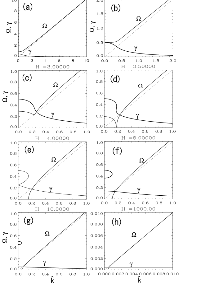
Figure 1: Dispersion relation for electromagnetic waves in the resistive pair plasma for various $H$. The dotted line shows the dispersion relation for electromagnetic waves in vacuum.

Figure 2: Dependence of $\hat{k}_{\rm crit}$ on $H$. At $\hat{k}=\hat{k}_{\rm crit}+0$, $\partial\Omega/\partial\hat{k}$ becomes infinity for each $H$.

We now show that matter composed of electrons and positrons with $H\geq 1$ cannot be treated as a plasma. This means that superluminal propagation of electromagnetic waves is not permitted when the medium is a plasma; and, when it is not, the medium must be treated in a different manner. Note that in this paragraph only, we shall use the SI unit system. The plasma parameter is given by

$$N_{\rm p}=n\lambda_{\rm D}^{3}=\sqrt{\frac{(\epsilon_{0}T)^{3}}{ne^{6}}},$$ (40)

where $T$ is the temperature of the electron/positron fluids and $\lambda_{\rm D}$ is the Debye length, $\lambda_{\rm D}=\epsilon_{0}T/(ne^{2})$ bellan06 . For a plasma, $N_{\rm p}$ is (much) larger than unity because charged particles are bound to each other when $N_{\rm p}<1$. The frequency of electron–positron Coulomb collisions can be written as,

$$\nu_{\rm ee}=\frac{ne^{4}\ln\Lambda}{6\sqrt{3}\pi\epsilon_{0}^{2}\sqrt{m}T^{3/2}}=\frac{ne^{4}}{\epsilon_{0}^{2}\sqrt{m}T^{3/2}}\ln\Lambda^{\prime},$$ (41)

where $\ln\Lambda$ is the Coulomb logarithm and $\ln\Lambda^{\prime}=\ln\Lambda/(6\sqrt{3}\pi)\sim 1/3$ bellan06 . Here we used $\ln\Lambda\sim 10$. Then we find that $H=2(mn/h)(\nu_{\rm ee}/\omega_{\rm pe})^{2}<2(\nu_{\rm ee}/\omega_{\rm pe})^{2}=2(\ln\Lambda)^{2}ne^{6}/(\epsilon_{0}T)^{3}$. Finally, we get the relation between $H$ and $N_{\rm p}$,

$$HN_{\rm p}^{2}<2(\ln\Lambda^{\prime})^{2}\sim\frac{2}{9}.$$ (42)

Therefore, when we consider a plasma (i.e., $N_{\rm p}>1$), we find that $H<(\ln\Lambda^{\prime})^{2}/N_{\rm p}^{2}\lesssim 2/9<1$. This clearly shows superluminal propagation of electromagnetic wave is not permitted in a true plasma (usually, $N_{\rm p}\gg 1$).

In the above discussion we used the rough approximation $\ln\Lambda\sim 10$. If $\ln\Lambda$ were greater than 100 separately with other variables, $H$ would become larger than 3 and then superluminal communication would become possible. However, this situation can never be realized because there is strict relation between $\Lambda$ and $N_{\rm p}$ as $\Lambda=6\pi N_{\rm p}$ (see bellan06 , page 24). So, if $\ln\Lambda$ becomes larger, then $N_{\rm p}$ becomes much larger and $H$ decreases to a value much less than unity.

Next, we discuss briefly the dispersion relation for electromagnetic waves in a uniformly magnetized pair plasma. We assume the background plasma is the same as that of the previous unmagnetized case except for a uniform magnetic field, $\mbox{\boldmath$B$}=\mbox{\boldmath$B$}_{0}\neq\mbox{\boldmath$0$}$. Using the same procedure employed in the previous unmagnetized plasma case, we obtain the linearized equations,

$$\mbox{\boldmath$E$}_{1}+\frac{i}{\omega h_{0}}(\mbox{\boldmath$J$}_{1}\times\mbox{\boldmath$B$}_{0})\times\mbox{\boldmath$B$}_{0} = (\eta-i\kappa\omega)\mbox{\boldmath$J$}_{1},$$ (43)

$$\omega^{2}\mbox{\boldmath$E$}_{1}+i\omega\mbox{\boldmath$J$}_{1}=k^{2}\mbox{\boldmath$E$}_{1},$$ (44)

where we assume $\mbox{\boldmath$k$}\cdot\mbox{\boldmath$V$}_{1}=0$ and $\mbox{\boldmath$k$}\cdot\mbox{\boldmath$E$}_{1}=0$ to investigate transverse modes. When we separate the perturbations of the electric field and current density into two components parallel and perpendicular to the background magnetic field $\mbox{\boldmath$B$}_{0}$,

$$\mbox{\boldmath$E$}_{1}=\mbox{\boldmath$E$}_{\parallel}+\mbox{\boldmath$E$}_{\perp}, \mbox{\boldmath$E$}_{\parallel}\parallel\mbox{\boldmath$B$}_{0}, \mbox{\boldmath$E$}_{\perp}\perp\mbox{\boldmath$B$}_{0},$$ (45)

$$\mbox{\boldmath$J$}_{1}=\mbox{\boldmath$J$}_{\parallel}+\mbox{\boldmath$J$}_{\perp}, \mbox{\boldmath$J$}_{\parallel}\parallel\mbox{\boldmath$B$}_{0}, \mbox{\boldmath$J$}_{\perp}\perp\mbox{\boldmath$B$}_{0},$$ (46)

equations (43) and (44) yield

$$\mbox{\boldmath$E$}_{\perp}-\frac{iB_{0}^{2}}{\omega h_{0}}\mbox{\boldmath$J$}_{\perp} = (\eta-i\kappa\omega)\mbox{\boldmath$J$}_{\perp},$$ (48)

$$(k^{2}-\omega^{2})\mbox{\boldmath$E$}_{\perp} = i\omega\mbox{\boldmath$J$}_{\perp},$$ (49)

$$\mbox{\boldmath$E$}_{\parallel} = (\eta-i\kappa\omega)\mbox{\boldmath$J$}_{\parallel},$$ (50)

$$(k^{2}-\omega^{2})\mbox{\boldmath$E$}_{\parallel} = i\omega\mbox{\boldmath$J$}_{\parallel}.$$ (51)

Finally, we obtain the two dispersion relations,

$$(k^{2}-\omega^{2})\left(\eta-i\kappa\omega+\frac{iB_{0}^{2}}{\omega h_{0}}\right) = i\omega,$$ (53)

$$(k^{2}-\omega^{2})(\eta-i\kappa\omega) = i\omega.$$ (54)

Equations (53) and (54) are not satisfied simultaneously when $B_{0}\neq 0$. Equation (54) is the same as that of the unmagnetized pair plasma case. Therefore, we shall investigate the dispersion relation (53).

When we set $\hat{\omega}=\kappa\omega/\eta$, $\hat{k}=\kappa k/\eta$, we have,

$$H(\hat{\omega}^{2}-\hat{k}^{2})(i\hat{\omega}+\hat{\omega}^{2}-\alpha)=\omega^{2},$$ (55)

where $H=\eta^{2}/\kappa$ and $\alpha=B_{0}^{2}\kappa/(h_{0}\eta^{2})=u_{\rm A}^{2}/H$ ($u_{\rm A}\equiv B_{0}/\sqrt{h_{0}}$ is the Alfven four-velocity). Setting $\hat{\omega}=\Omega-i\gamma$ ($\Omega\geq 0,\gamma\in{\bf R}$), we obtain the dispersion relation for electromagnetic waves in a magnetized pair plasma,

$$H[(\Omega^{2}-\gamma^{2}-\hat{k}^{2})(\Omega^{2}-\gamma^{2}-\alpha+\gamma)+2\Omega^{2}\gamma(1-2\gamma)] = \Omega^{2}-\gamma^{2},$$ (56)

$$H[(\Omega^{2}-\gamma^{2}-\hat{k}^{2})(1-2\gamma)-2\gamma(\Omega^{2}-\gamma^{2}-\alpha+\gamma)] = -2\gamma,$$ (57)

where we assume $\Omega\neq 0$. Figure 3 shows the dispersion relation for $\Omega$ in the case $H=1$ and $\alpha=0.1,1$. The figure clearly shows the group velocity of electromagnetic waves in a magnetized pair plasma is less than the light speed in vacuum when $H=1$. A detailed investigation shows that this is true when $H<1$ as in the unmagnetized pair plasma case. However, when $H>4$, the group velocity is larger than the speed of light for some ranges of $\hat{k}$.

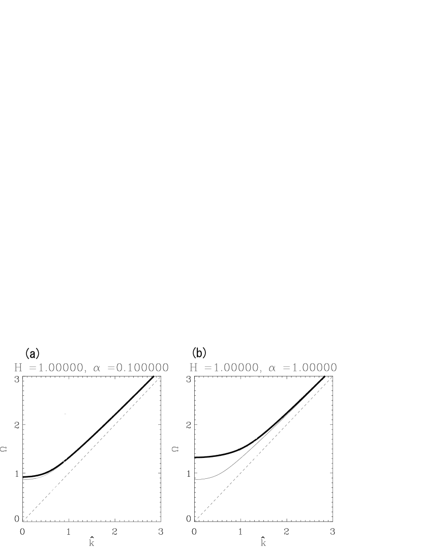
Figure 3: The dispersion relation of electromagnetic waves in uniform, magnetized pair plasma (thick solid lines) and in unmagnetized plasma for comparison ($\alpha=0$; thin solid lines). (a) Sub-relativistically strong magnetic field case, $H=1$, $\alpha=0.1$. (b) Relativistically strong magnetic field case, $H=1$, $\alpha=1$.

IV Causal Resistive RMHD Equations

In the above discussion, we derived the one-fluid equations (19)–(26) from the two-fluid ones. The one-fluid equations confirmed that the superluminal propagation is forbidden in a two-component medium that has a plasma whose plasma parameter greater than unity. That is, the one-fluid equations of a pair plasma (19)–(26) are causal. When we neglect the first term of the right hand side in Ohm’s law equation (21), which comes from the inertial effect of the positron and electron, the term, $-i\omega/(2\nu^{\prime}_{\rm ee})$, on the left hand side of the dispersion relation (35) drops out. In this case, the group velocity becomes $v_{\rm g}=\partial\omega/\partial k=2k(4k^{2}-\eta^{-2})^{-1/2}>1$, which means the group velocity is greater than the speed of light (superluminal). As shown in Appendix C, when the group velocity is larger than the speed of light, superluminal communication would become possible, allowing us to develop a device that could send information into the past. However, such a device would destroy the causality of time–ordered events and, therefore, should not be possible. This means that, in order to preserve causality, we cannot neglect the inertial term of the electron and positron in Ohm’s law (21). Recently, several groups performed simulations of resistive RMHD including Ohm’s law without the electron/positron inertia effect watanabe06 ; komissarov07b . As shown in the above results, unfortunately, all of these calculations are acausal. Here, we propose a set of causal resistive RMHD equations in a simple form.

For simplicity, assuming that $|\Delta\tilde{h}|\ll\tilde{h}$ and $p_{+}\approx p_{-}$, we obtain the following equations,

$$\frac{\partial}{\partial t}(\gamma\rho)+\nabla\cdot(\rho\mbox{\boldmath$U$}) = 0,$$ (58)

$$\frac{\partial}{\partial t}\left[\tilde{h}\left(\gamma\mbox{\boldmath$U$}+\frac{\rho_{\rm e}}{(2ne)^{2}}\mbox{\boldmath$J$}\right)\right]+\nabla\cdot\left[\tilde{h}\left(\mbox{\boldmath$UU$}+\frac{1}{(2ne)^{2}}\mbox{\boldmath$JJ$}\right)\right] = -\nabla p+\rho_{\rm e}\mbox{\boldmath$E$}+\mbox{\boldmath$J$}\times\mbox{\boldmath$B$},$$ (59)

$$\frac{\partial}{\partial t}\left[\tilde{h}\left(\gamma^{2}+\frac{\rho_{\rm e}^{2}}{(2ne)^{2}}\right)-p\right]+\nabla\cdot\left[\tilde{h}\left(\gamma\mbox{\boldmath$U$}+\frac{\rho_{\rm e}}{(2ne)^{2}}\mbox{\boldmath$J$}\right)\right] = \mbox{\boldmath$J$}\cdot\mbox{\boldmath$E$},$$ (60)

$$\mbox{\boldmath$E$}+\mbox{\boldmath$V$}\times\mbox{\boldmath$B$}-\frac{\eta}{\gamma}[\mbox{\boldmath$J$}-\gamma^{2}(\rho_{\rm e}-\mbox{\boldmath$V$}\cdot\mbox{\boldmath$J$})(1+\Theta)\mbox{\boldmath$V$}]$$

$$=\frac{1}{4ne\gamma}\left[\frac{\partial}{\partial t}\left(\frac{\tilde{h}}{ne}(\gamma\mbox{\boldmath$J$}+\rho_{\rm e}\mbox{\boldmath$U$})\right)+\nabla\cdot\left\{\frac{\tilde{h}}{ne}(\mbox{\boldmath$UJ$}+\mbox{\boldmath$JU$})\right\}\right],$$ (61)

$$\nabla\cdot\mbox{\boldmath$E$} = \rho_{\rm e},$$ (62)

$$\nabla\cdot\mbox{\boldmath$B$} = 0,$$ (63)

$$\frac{\partial\mbox{\boldmath$B$}}{\partial t} = -\nabla\times\mbox{\boldmath$E$},$$ (64)

$$\frac{\partial\mbox{\boldmath$E$}}{\partial t}+\mbox{\boldmath$J$} = \nabla\times\mbox{\boldmath$B$},$$ (65)

where $\Theta=2\theta(m/e)^{2}(Q^{2}+W)\left/\left[\rho^{2}-\left(mQ/e\right)^{2}\right]\right.$ (see Appendix A). Here we have to assume $\gamma^{\prime}\approx 1$ and $M=U_{\nu}U^{\nu}=-1$ in Appendix A, which means that the relative velocity of the electron fluid and positron fluid is nonrelativistic. This condition also preserves $\gamma=1/(1-V^{2})^{1/2}$. In a pair plasma, we use $\theta=1$.

A covariant form for these one-component fluid equations (58)–(65) is as follows:

$$\partial_{\nu}(\rho U^{\nu}) = 0,$$ (66)

$$\partial_{\nu}\left[\tilde{h}\left(U^{\nu}U^{\mu}+\frac{1}{(2ne)^{2}}J^{\nu}J^{\mu}\right)\right] = -\partial^{\mu}p+J^{\nu}F_{\nu}^{\mu},$$ (67)

$$U^{\nu}F_{\nu}^{\mu}-\eta[J^{\mu}+(U^{\nu}J_{\nu})(1+\Theta)U^{\mu}] = \frac{1}{4ne^{2}}\left[\partial_{\nu}\left\{\frac{\tilde{h}}{n}\left(U^{\nu}J^{\mu}+J^{\nu}U^{\mu}\right)\right\}\right],$$ (68)

$$\partial_{\nu}F^{\nu\mu} = J^{\mu},$$ (69)

$$\partial_{\nu}\hskip 3.00003pt^{*}F^{\nu\mu} = 0.$$ (70)

The difference between equations (58)–(65) and the RMHD equations used by the previous acausal resistive RMHD simulations watanabe06 ; komissarov07b is mainly in Ohm’s law, as expected and suggested by other articles ardavan76 ; blackman93 ; gedalin96 ; melatos96 ; khanna98 ; meier04 . The linear analysis of the electromagnetic wave in a pair plasma shows that the inertia effect of the electron and positron is essential in preserving causality. Here, the electron/positron inertia term of Ohm’s law is the right hand side of equation (61). If we neglect the change of $\gamma h/n$, Ohm’s law simplifies to

$$\mbox{\boldmath$E$}+\mbox{\boldmath$V$}\times\mbox{\boldmath$B$}-\frac{\eta}{\gamma}[\mbox{\boldmath$J$}-\gamma^{2}(\rho_{\rm e}-\mbox{\boldmath$V$}\cdot\mbox{\boldmath$J$})(1+\Theta)\mbox{\boldmath$V$}]=\kappa\left[\frac{\partial}{\partial t}(\mbox{\boldmath$J$}+\rho_{\rm e}\mbox{\boldmath$V$})+\nabla\cdot\left(\mbox{\boldmath$VJ$}+\mbox{\boldmath$JV$}\right)\right],$$ (71)

where $\kappa=\tilde{h}/(2en)^{2}$. When $H=\eta^{2}/\kappa<1$, that is $\eta<\sqrt{\kappa}$, equations (58)–(60), (62)–(65), (71) are causal, and thus we call equations (58)–(60), (62)–(65),(71) with $\eta<\sqrt{\kappa}$ the “causal resistive RMHD” equations. Among the causal resistive RMHD equations, equation (71) is most important; we call it the “causal Ohm’s law”. When we set $\Theta=0$ , equation (71) reduces to the simpler Ohm’s law,

$$\mbox{\boldmath$E$}+\mbox{\boldmath$V$}\times\mbox{\boldmath$B$}-\frac{\eta}{\gamma}\left[\mbox{\boldmath$J$}-\gamma^{2}(\rho_{\rm e}-\mbox{\boldmath$V$}\cdot\mbox{\boldmath$J$})\mbox{\boldmath$V$}\right]=\kappa\left[\frac{\partial}{\partial t}(\mbox{\boldmath$J$}+\rho_{\rm e}\mbox{\boldmath$V$})+\nabla\cdot\left(\mbox{\boldmath$VJ$}+\mbox{\boldmath$JV$}\right)\right],$$ (72)

which is quite similar to the generalized Ohm’s law derived by ardavan76 and meier04 , but not identical.

V Expected Phenomena related to superluminal wave packet

In this section, we discuss phenomena related to superluminal propagation of electromagnetic wave packets that appeared in RMHD simulations that use an acausal Ohm’s law with $H=\eta^{2}/\kappa\gtrsim 3$. First, we show that it is difficult to detect the superluminal propagation of a electromagnetic wave packet in an unmagnetized plasma at rest. For simplicity, we use the acausal Ohm’s law with $\kappa=0$ ($H\rightarrow\infty$). This is just the case of the previous studies with resistive RMHD watanabe06 ; komissarov07b . In this case, the dispersion relation becomes that of the telegraphic equation,

$$\omega^{2}+\frac{i}{\eta}\omega-k^{2}=0.$$ (73)

The group velocity of the dispersion relation $v_{\rm g}=\partial\omega/\partial k=k/[k^{2}-(2\eta)^{-2}]^{1/2}>1$ is always greater than the light speed in vacuum. The damping time of the wave is $\tau_{\rm damp}=1/(-\Im(\omega))=2\eta$. The diffusion time of the wave packet is calculated by

$$\tau_{\rm diff}=\frac{\sigma^{2}}{|D|}=\frac{\sigma^{2}}{|\partial^{2}\omega/\partial k^{2}|}=\sigma^{2}(2\eta)^{2}[k^{2}-(2\eta)^{-2}]^{3/2},$$

where $\sigma$ is the width of the wave packet (see Appendix C, equation (120)). The life time of the wave packet is estimated by

$$\tau=\left(\frac{1}{\tau_{\rm damp}}+\frac{1}{\tau_{\rm diff}}\right)^{-1}=\frac{\sigma^{2}(2\eta)^{2}[k^{2}-(2\eta)^{-2}]^{3/2}}{1+\sigma^{2}(2\eta)[k^{2}-(2\eta)^{-2}]^{3/2}}.$$ (74)

The characteristic propagation length of the wave packet is

$$l=v_{\rm g}\tau=\frac{k\sigma^{2}(2\eta)^{2}[k^{2}-(2\eta)^{-2}]}{1+\sigma^{2}(2\eta)[k^{2}-(2\eta)^{-2}]^{3/2}}.$$

Using $N=k\sigma$ and $\chi=2\eta k$, we have

$$\frac{l}{\sigma}=\frac{N\chi^{2}(\chi^{2}-1)}{\chi^{2}+N^{2}(\chi^{2}-1)^{3/2}}.$$ (75)

Note that the limitation $l/\sigma\rightarrow\infty$ ($\chi\rightarrow\infty$) means the wave packet propagates to a very long distance compared to the scale of the wave packet itself in a highly resistive plasma, where the situation is almost the same in a vacuum. However, to detect the superluminal propagation of the wave packet, we have to detect the difference between the propagation length of the wave packet and that of the light in vacuum, $\Delta l=l-\tau$. The difference is estimated as

$$\frac{\Delta l}{\sigma}=\frac{l}{\sigma}\left(1-\frac{1}{v_{\rm g}}\right)=\frac{N(\chi^{2}-1)}{[N^{2}(\chi^{2}-1)^{3/2}+\chi^{2}]\left(1+\sqrt{1-\chi^{-2}}\right)}\leq\frac{2^{2/3}N}{3N^{4/3}+2^{2/3}}.$$ (76)

Because $N\gg 1$, equation (76) shows $\Delta l\ll\sigma$. This means detection of the superluminal propagation of the wave packet is difficult in the rest background plasma with a detector of ordinary sensitivity.

When we consider a moving plasma with relativistic speed, propagation of the superluminal wave packet changes drastically. Here we consider the wave packet propagating along the $x$ direction of a frame $(t,x)$ in a uniform, unmagnetized plasma at rest (see Fig. 4(a)). We assume that the wave packet propagates with the group velocity $v_{\rm g}>1$ and damps with the damping rate $\gamma_{\rm dmp}$. Next, we consider a new frame $(t^{\prime},x^{\prime})$ moving with velocity $v_{0}>1/v_{\rm g}$ relative to the frame $(t,x)$, where the $t^{\prime}$-axis and $x^{\prime}$-axis in the space-time $(t,x)$ are drawn as shown in Fig. 4(a). The world line of the wave packet is located between the $x^{\prime}$-axis and $x$-axis. When we ride on the new frame $(t^{\prime},x^{\prime})$, we see from time inversion arguments that the wave packet propagates from the right to the left as shown in Fig. 4(b). Furthermore, the wave packet grows at the rate $\gamma^{\prime}_{\rm grw}=\gamma_{\rm dmp}\sqrt{1-v_{0}^{2}}/(v_{0}v_{\rm g}-1)$. Here the points A, B, and C with respect to the wave packet are identified with those at A’, B’, and C’, respectively. This suggests that we have to use the causal RMHD equations (58)–(60), (62)–(65), and (71) to avoid such a strange instability of the wave packet, at least in relativistic plasma flow, because wave packets propagating in such a flow will grow explosively. Relativistic flow exists around the black hole horizon in the Kerr space-time, so artificial radiation of electromagnetic wave packets from the horizon will occur in acausal RMHD calculations. On the other hand, the same acausal RMHD equations with $\kappa=0$ cause no problem for a non-relativistically moving plasma.

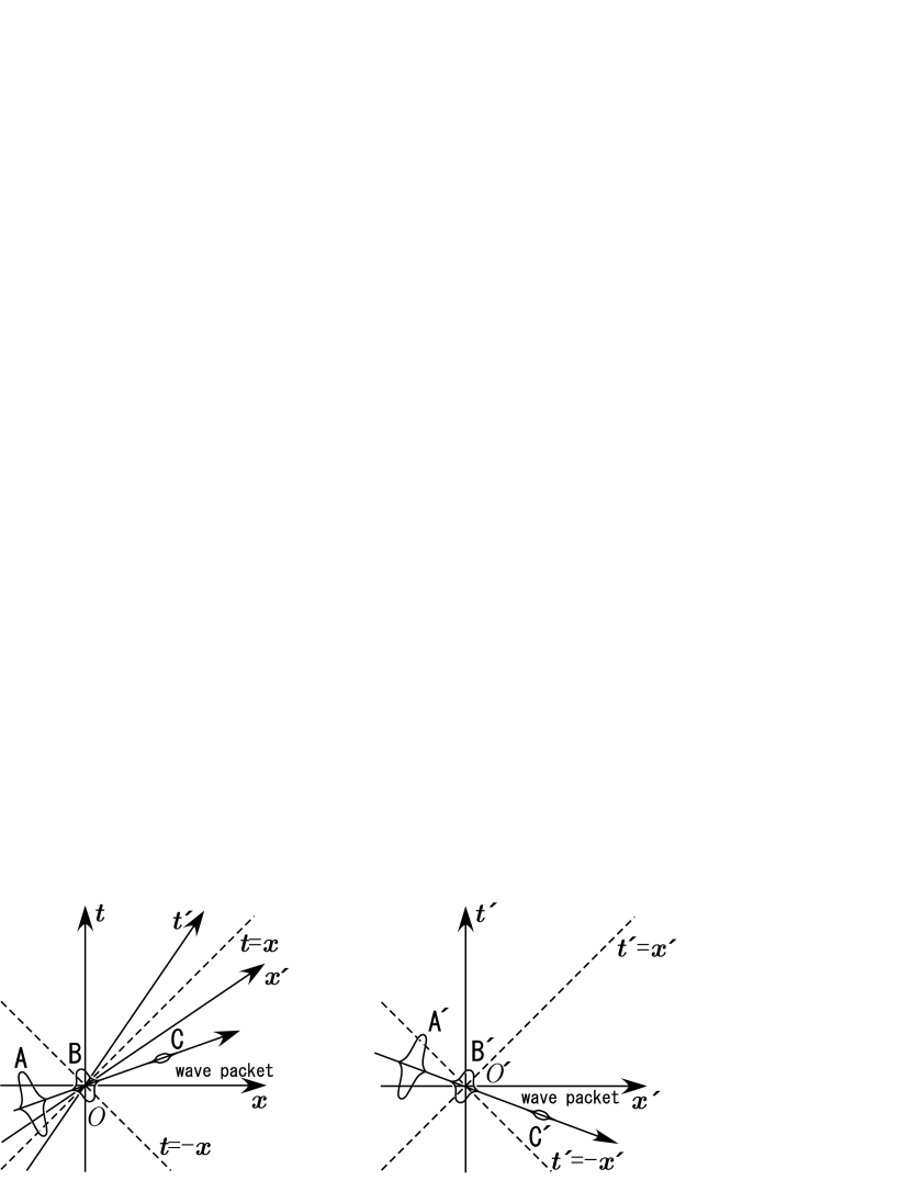
Figure 4: Propagation of electromagnetic wave packet in the uniform, unmagnetized plasma. (a) Case of rest plasma. (b) Case of relativistic flow of plasma.

VI Concluding Remarks and Discussion

We have derived the dispersion relation for electromagnetic waves in a resistive pair plasma based on the relativistic two-fluid model, and have shown that the group velocity of electromagnetic waves in a resistive plasma is smaller than the light speed within the plasma condition ($N_{\rm p}>1$). This shows that superluminal communication is impossible in a resistive plasma, thus confirming the causal nature of signals in plasmas. Furthermore, the causality condition, $H=\eta^{2}/\kappa<2(3N_{\rm p})^{-2}<1$, provides an upper limit for electric resistivity in resistive RMHD:

$$\eta<\sqrt{\kappa}=\sqrt{\frac{h_{0}}{2mc^{2}n_{0}}}\frac{1}{\epsilon_{0}\omega_{\rm pe}}=0.2\left(\frac{n_{\rm 0}}{10^{20}{\rm m}^{-3}}\right)^{-1/2}\left(\frac{h_{0}}{2mc^{2}n_{0}}\right)^{1/2}\,[\Omega\,{\rm m}].$$ (77)

For simplicity, we assumed that the relative velocity of the positron and electron fluids is much smaller than their internal thermal velocities. This is consistent with the assumption of linear analysis. In general, however, this assumption is not valid, especially for relativistic plasma around black holes. To deal with plasmas where the relative velocity of the electron and positron fluids is relativistic, we have to return to the relativistic Vlasov–Boltzmann equation with collisional terms ardavan76 ; blackman93 ; gedalin96 ; meier04 to obtain the resistive term in the causal Ohm’s law. In such a case, resistivity depends on current density.

We emphasize that the inertia effect is important for preserving causality, i.e., to forbid the superluminal propagation of electromagnetic waves in a resistive plasma. If we neglect the inertia term in the generalized Ohm’s law (the first term of the right hand side of equation (21)), then the resistive RMHD equations give a group velocity of electromagnetic waves, $v_{\rm g}=\partial\omega/\partial k=2k/(4k^{2}-\eta^{-2})^{1/2}$, that is greater than the light speed. This shows that the inertia effects of electrons and positrons should be considered to preserve causality. We therefore proposed a set of causal resistive RMHD equations in section IV. Numerical techniques for simulating “causal resistive RMHD” flow should be developed quickly and be applied to astrophysical calculations —– e.g., energy extraction from a rotating black hole by magnetic reconnection koide08 . To perform causal resistive RMHD simulations of a black hole magnetosphere, we are to use the general relativistic MHD equations along with the causal Ohm’s law.

When we consider matter with a plasma parameter less than one, we cannot use the simple two-fluid approximation, because particles in the system are electrically bound to each other. Metal, like iron, is an example for such matter. To treat such a relativistic system, we ultimately must use relativistic quantum mechanics. However, we have no framework for that at present; nevertheless it is an interesting and challenging field for future work. In such an unknown framework, the group velocity of electromagnetic waves in any medium should not be larger than the light speed (even if the wave damps quickly) to preserve causality. On the other hand, within the classical framework where we neglect quantum effects, we would show that the group velocity is always equal to or smaller than the speed of light when we treat the system properly. Here we cannot use the method of smoothing the electromagnetic field, as is done in traditional particle simulations, because the simple smoothing destroys causality. Therefore, numerical calculations may be more difficult than traditional plasma particle simulations. It is interesting and important to investigate, in a medium with a small plasma parameter, which effects (quantum or classical effects) are more important for keeping the group velocity of electromagnetic wave equal to or less than the speed of light.

In this paper, we considered only a pair plasma; we did not treat an electron–proton plasma. However, the similar conclusions also should be drawn for the latter (at lease when the plasma is unmagnetized), because the linearized terms of resistive RMHD in a pair plasma and in an electron–proton plasma are expected to be similar. It also is important to note the differences between RMHD of a pair plasma and in an electron–proton plasma. These come from the inequality between the mass ratios of the electron–positron and electron–proton. With respect to equations (58)–(60), (62)–(65), (71), it is expected that these equations are similar except for appearance of the second term in the brackets on the left hand side of equation (59), $\mbox{\boldmath$JJ$}/(2ne)^{2}$, and the term in the brackets on the left hand side of equation (71), $\gamma^{2}(\rho_{\rm e}-\mbox{\boldmath$V$}\cdot\mbox{\boldmath$J$})\Theta\mbox{\boldmath$V$}$. In the electron–proton plasma, the electron inertia term with $JJ$ is negligible compared to the proton inertia term with $UU$, and $\Theta$ vanishes because of poor energy exchange between the electron and proton fluids. However, in the pair plasma, $\Theta$ is not negligible. Furthermore, the Hall effect disappears in Ohm’s law (71) in the pair plasma case. Note that all of the terms are nonlinear and that the coefficient $\kappa$ of the inertia term in the causal Ohm’s law for the electron–proton plasma is much smaller than that of the pair plasma (by the ratio of the electron and proton masses). It is believed that an accretion disk in a black hole magnetosphere of an AGN will consist of an electron–proton plasma and a corona around the disk and a relativistic jet from AGN consist of pair plasma wardle98 . Comparison between phenomena in relativistic pair plasmas and electron–proton plasmas is both interesting and necessary for understanding the physics of black hole magnetospheres where a relativistic jet may be produced.

Appendix A Derivation of frictional four-force density

In this appendix, we derive the friction four-force density between electron and positron fluids, whose proper densities are $n_{\pm}$. We use $f_{-}^{\mu}$ and $f_{+}^{\mu}$ to denote the friction density of the electron and positron fluids, respectively. The principle of action–reaction is expressed as

$$f_{+}^{i}+f_{-}^{i}=0\verb! !(i=1,2,3),$$ (78)

in any inertial frame $x^{\mu}$. When we consider any other inertial frame $X^{\mu}=A^{\mu}_{\nu}x^{\nu}$, the principle of action and reaction is

$$F_{+}^{i}+F_{-}^{i}=A^{i}_{\nu}(f_{+}^{\nu}+f_{-}^{\nu})=A^{i}_{0}(f_{+}^{0}+f_{-}^{0})=0.$$ (79)

Because $A^{i}_{0}\neq 0$ in general, we have $f_{+}^{0}+f_{-}^{0}=0$, or

$$f_{+}^{\mu}+f_{-}^{\mu}=0.$$ (80)

Note that $f_{+}^{0}+f_{-}^{0}=0$ is the law of conservation of energy. We consider the center-of-mass frame of the two fluids $x^{\mu^{\prime}}=a^{\mu}_{\nu}x^{\nu}$ where the four-velocity of the electron/positron fluids $U_{\pm}^{\mu^{\prime}}$ satisfies

$$n_{+}U_{+}^{i^{\prime}}+n_{-}U_{-}^{i^{\prime}}=0.$$ (81)

With respect to the inverse transformation, $x^{\mu}=b^{\mu}_{\nu}x^{\nu\prime}$, we have

$$n_{+}U_{+}^{\mu}+n_{-}U_{-}^{\mu}=b^{\mu}_{\nu}(n_{+}U_{+}^{\nu\prime}+n_{-}U_{-}^{\nu\prime})-b^{\mu}_{0}(n_{+}\gamma_{+}^{\prime}+n_{-}\gamma_{-}^{\prime}),$$ (82)

where the prime denotes the variable observed in the center-of-mass frame. Using the definition $U^{\mu}=(n_{+}U_{+}^{\mu}+n_{-}U_{-}^{\mu})/(2n)$ and $\gamma=(n_{+}\gamma_{+}+n_{-}\gamma_{-})/(2n)$, we have

$$b^{\mu}_{0}=\frac{U^{\mu}}{\gamma^{\prime}}.$$ (83)

In the center-of-mass frame, the spacial components of the friction force density are

$$-f_{-}^{i^{\prime}}=f_{+}^{i^{\prime}}=-m\sigma_{\rm ee}v_{\rm r}n_{+}n_{-}\gamma_{+}^{\prime}\gamma_{-}^{\prime}(v_{+}^{i\prime}-v_{-}^{i\prime}),$$ (84)

where $\sigma_{\rm ee}$ is the electron/positron collisional cross section, which is a function of the thermal velocity. The average relative velocity of the electrons and positrons, $v_{\rm r}$, is roughly given by the maximum of the thermal velocity and the relative velocity of the two fluids. We write the friction four-force density as

$$-f_{-}^{\mu}=f_{+}^{\mu}=b^{\mu}_{\nu}f_{+}^{\nu\prime} = -m\sigma_{\rm ee}v_{\rm r}n_{+}n_{-}\gamma_{+}^{\prime}\gamma_{-}^{\prime}(v_{+}^{i\prime}-v_{-}^{i\prime})+b^{\mu}_{0}f_{+}^{0\prime}$$ (85)

$$= -m\sigma_{\rm ee}v_{\rm r}(n_{-}\gamma_{-}^{\prime}n_{+}U_{+}^{\mu}-n_{+}\gamma_{+}^{\prime}n_{-}U_{-}^{\mu})+b^{\mu}_{0}f_{+}^{0\prime}.$$

When we use the collision frequency of the electron and positron $\nu_{\rm ee}=\sigma_{\rm ee}v_{\rm r}n$ and equation (83), we have

$$f_{+}^{\mu}=-\frac{m\nu_{\rm ee}}{n}(n_{-}\gamma_{-}^{\prime}n_{+}U^{\mu}_{+}-n_{+}\gamma_{+}^{\prime}n_{-}U^{\mu}_{-})+\frac{n_{+}U^{\mu}_{+}+n_{-}U^{\mu}_{-}}{n_{+}\gamma_{+}^{\prime}+n_{-}\gamma_{-}^{\prime}}f_{+}^{0\prime}.$$ (86)

Next we consider the energy gain rate of the positron fluid $f_{+}^{0\prime}$ in the center-of-mass frame. The positron and electron fluids lose the kinetic energy due to friction at the rate,

$$-f_{+}^{i\prime}v_{+i}^{\prime}-f_{-}^{i\prime}v_{-i}^{\prime} = -f_{+}^{i\prime}v_{+i}^{\prime}-\frac{1}{n_{-}\gamma_{-}^{\prime}}f_{-}^{i\prime}n_{-}U_{-i}^{\prime}$$ (87)

$$= -f_{+}^{i\prime}v_{+i}^{\prime}-\frac{1}{n_{-}\gamma_{-}^{\prime}}f_{+}^{i\prime}n_{+}U_{+i}^{\prime}=-f_{+}^{i\prime}v_{+i}^{\prime}\left(1+\frac{n_{+}\gamma_{+}^{\prime}}{n_{-}\gamma_{-}^{\prime}}\right).$$

In the above calculation, we employ the principle of action–reaction (80), the condition of the center-of-mass frame (81), and the assumption that the lost energy is thermalized. A fraction $\theta$ of this thermalized energy ($0\leq\theta\leq 1$) is distributed to the positron and electron fluids, assuming equipartition, and other part is returned to the original fluid. Then the energy gain rate of the positron is calculated as

$$f_{+}^{0\prime} = \frac{-\theta f_{+}^{i\prime}v_{+i}^{\prime}-\theta f_{-}^{i\prime}v_{-i}^{\prime}}{\gamma_{+}^{\prime}n_{+}+\gamma_{-}^{\prime}n_{-}}\gamma_{+}^{\prime}n_{+}+(1-\theta)(-f_{+}^{i\prime}v_{+i}^{\prime})-(-f_{+}^{i\prime}v_{+i})$$ (88)

$$= -\theta f_{+}^{i\prime}v_{+i}\frac{\gamma_{+}^{\prime}n_{+}-\gamma_{-}n_{-}}{n_{-}\gamma_{-}^{\prime}}.$$ (89)

Using the definition of the average four-velocity and four-current density (15), (16) and the friction force density expression (86), we have

$$f_{+}^{i\prime}v_{+i}^{\prime} = -m\sigma_{\rm ee}v_{\rm r}n_{+}n_{-}\gamma_{+}^{\prime}\gamma_{-}^{\prime}(v_{+}^{i\prime}-v_{-}^{i\prime})v_{+i}^{\prime}$$ (90)

$$= -\frac{m\sigma_{\rm ee}v_{\rm r}n}{2n_{+}\gamma_{+}^{\prime}\gamma^{\prime}e^{2}}[Q^{2}-WM],$$

where $M=U_{\nu}U^{\nu}$, $Q=J_{\nu}U^{\nu}$, $W=J_{\nu}J^{\nu}$. Equations (89) and (90) yield

$$f_{+}^{0\prime} = \frac{m\sigma_{\rm ee}v_{\rm r}n}{2e^{2}n_{+}\gamma_{+}^{\prime}\gamma^{\prime}n_{-}\gamma_{-}^{\prime}}(Q^{2}-WM)(\gamma_{+}^{\prime}n_{+}-\gamma_{-}^{\prime}n_{-})\theta$$ (91)

$$= -\frac{m\sigma_{\rm ee}v_{\rm r}n^{2}/e^{2}}{(n^{2}M)^{2}-\left(\frac{n}{2e}Q\right)^{2}}(Q^{2}-WM)\frac{nQ}{2e}\theta.$$

Here we used

$$\gamma_{+}^{\prime}n_{+}-\gamma_{-}n_{-}^{\prime} = \gamma^{\prime}J^{0\prime}=-J^{0\prime}U_{0}^{\prime}=-J^{\nu\prime}U_{\nu}^{\prime}=-J^{\nu}U_{\nu}=-Q,$$

$$\gamma^{\prime 2} = -U^{0\prime}U_{0}^{\prime}=-U^{\nu\prime}U_{\nu}^{\prime}=-U^{\nu}U_{\nu}=-M,$$

$$\gamma^{\prime 2}n_{+}\gamma_{+}^{\prime}n_{-}\gamma_{-}^{\prime} = \gamma^{\prime 2}\left(nU^{0\prime}+\frac{J^{0\prime}}{2e}\right)\left(nU^{0\prime}-\frac{J^{0\prime}}{2e}\right)$$ (92)

$$= \frac{1}{n^{2}}\left[(n^{2}U_{\nu}U^{\nu})^{2}-\left(\frac{n}{2e}J_{\nu}U^{\nu}\right)^{2}\right].$$

The equation of friction four-force density (86) reads

$$f_{+}^{\mu} = -m\sigma_{\rm ee}v_{\rm r}\left[n_{-}\gamma_{-}^{\prime}\left(nU^{\mu}+\frac{1}{2e}J^{\mu}\right)-n_{+}\gamma_{+}^{\prime}\left(nU^{\mu}-\frac{1}{2e}J^{\mu}\right)\right]+\frac{U^{\mu}}{\gamma^{\prime}}f_{+}^{0\prime}$$ (93)

$$= -\frac{m\sigma_{\rm ee}v_{\rm r}n}{\gamma^{\prime}e}\left[-(U_{\nu}U^{\nu})J^{\mu}+(U_{\nu}J^{\nu})U^{\mu}\right]+\frac{U^{\mu}}{\gamma^{\prime}}f_{+}^{0\prime}.$$ (94)

When we introduce the dimensionless factor with respect to the left hand side of equation (91),

$$\Theta=\frac{2m^{2}}{e^{2}}\frac{Q^{2}-MW}{(2mnM)^{2}-(mQ/e)^{2}}\theta,$$ (95)

we finally obtain

$$f_{+}^{\mu}=-\frac{n\sigma_{\rm ee}v_{\rm r}n}{e}\sqrt{-M}\left[J^{\mu}-\frac{Q}{M}U^{\mu}(1+\Theta)\right].$$ (96)

We also calculate the resistive term in Ohm’s law,

$$\frac{f_{+}^{\mu}}{en\gamma}=-\eta\frac{\sqrt{-M}}{\gamma}\left[J^{\mu}-\frac{Q}{M}U^{\mu}(1+\Theta)\right],$$ (97)

where $\eta\equiv m\sigma_{\rm ee}v_{\rm r}/e^{2}$ is resistivity. When we use the collision frequency $\nu_{\rm ee}=\sigma_{\rm ee}v_{\rm r}n$, we can write $\eta=m\nu_{\rm ee}/(ne^{2})$.

Appendix B Forbidden range of superluminal communication

We prove that $\partial\Omega/\partial k<1$ in the dispersion relation (38) when $H<1.5$. In this appendix, we omit the hat over $\hat{k}$. The determinant of the cubic equation (37) with respect to $\gamma$ is $D_{\gamma}=-(C^{3}+F^{2})/(9\times 36^{2})$. If $\gamma$ had three different real solutions, it would yield $D_{\gamma}>0$, i.e., $\Omega^{2}(4\Omega^{2}-C)^{2}=(C^{3}+F^{2})/27<0$ ($\Omega$ would be pure imaginary). Then $\gamma$ has only one real solution, so that $\Omega$ has a real solution. When we consider a function of the left hand side of equation (37),

$$f(\gamma)=\gamma^{3}-\gamma^{2}-\frac{1}{4}\left(1+k^{2}+\frac{1}{H}\right)\gamma-\frac{1}{8H},$$

we have $f(0)=-1/(8H)<0$ and $f(1/2)=k^{2}/8>0$, and then the single solution of $\gamma$ should be $0<\gamma<1/2$. Then we have

$$k^{2}+\frac{1}{H}-\frac{1}{3}<\Omega^{2}<k^{2}+\frac{1}{H},$$ (98)

because

$$\Omega^{2}=3\gamma(\gamma-\frac{2}{3})+k^{2}+\frac{1}{H}=3\left(\gamma-\frac{1}{3}\right)^{2}-\frac{1}{3}+k^{2}+\frac{1}{H}.$$ (99)

From equation (39), we have

$$\Omega\frac{d\Omega}{dk}=(3\gamma-1)\frac{d\gamma}{dk}+k.$$ (100)

Using equation (37), we obtain

$$\frac{d\gamma}{dk}=k\left[1-\frac{1}{2}\frac{3\gamma^{2}-\gamma}{3\gamma^{2}-2\gamma+\frac{1}{4}(1+k^{2}+1/H)}\right].$$ (101)

When $H<3$, the denominator in equation (101) is positive because of the right side equation of equation (99). From equations (100) and (101), we have

$$\frac{d\Omega}{dk}=\frac{k}{2\Omega}\frac{\Omega^{2}-\frac{k^{2}}{2}-\frac{1}{2H}+\frac{1}{2}-\gamma}{\Omega^{2}-\frac{3k^{2}}{4}-\frac{3}{4H}+\frac{1}{4}}.$$ (102)

We consider the difference between the numerator and positive denominator of equation (102),

$$\Delta=k\left(\Omega^{2}-\frac{k^{2}}{2}-\frac{1}{2H}+\frac{1}{2}-\gamma\right)-2\Omega\left(\Omega^{2}-\frac{3k^{2}}{4})-\frac{3}{4H}+\frac{1}{4}\right).$$ (103)

After some algebraic calculations, we have

$$\Delta=(k-\Omega)\left(\Omega^{2}-k^{2}-\frac{1}{2H}\right)-\frac{\Omega}{4}\left(4\Omega^{2}-4k^{2}-\frac{4}{H}+2\right)+\left(\frac{1}{2}-\gamma\right)k-\frac{3}{4}\Omega k^{2}+(k-\Omega)\frac{k^{2}}{2}.$$ (104)

From the left inequality in equation (98), we find $\Omega>k$ when $H<3$. And then we have

$$\Delta\leq(k-\Omega)\left(\frac{1}{2H}-\frac{1}{3}\right)+(k-\Omega)\frac{k^{2}}{2}-\frac{\Omega}{6}+\left(\frac{1}{2}-\gamma\right)k-\frac{3}{4}k^{2}.$$ (105)

Using equation (39), we obtain

$$\Delta\leq(k-\Omega)\left(\frac{1}{2H}-\frac{1}{3}\right)+\frac{k-\Omega}{6}+\frac{k}{2}\left[\frac{2}{3}-\frac{1}{H}+\Omega\left(\Omega-\frac{5k}{2}\right)-3\gamma^{2}\right].$$ (106)

When $k\geq 2/\sqrt{21H}$, we get $\Omega^{2}<k^{2}+1/H\leq 25k^{2}/4$ using equation (98). Then we have $\Omega\geq 5k/2$ and $\Delta<0$ when $H<3/2$.

On the other hand, when $k<2/\sqrt{21H}$, we obtain $\Omega^{2}<k^{2}+1/H<25/(21H)$ and then $\Omega<5/\sqrt{21H}$. After some calculations, we have

$$\Delta \leq (\Omega-k)\left(\frac{1}{6}-\frac{1}{2H}+\frac{k\Omega}{2}-\frac{3k^{2}}{4}\right)+\frac{k}{2}\left(\frac{2}{3}-\frac{1}{H}\right)-\frac{3k^{2}}{4}-\frac{3\gamma^{2}k}{2}$$ (107)

$$< (\Omega-k)\left(\frac{1}{6}-\frac{11}{42H}-\frac{3k^{2}}{4}\right)+\frac{k}{2}\left(\frac{2}{3}-\frac{1}{H}\right)-\frac{3k^{2}}{4}-\frac{3\gamma^{2}k}{2}<0,$$

when $H\leq 3/2$. Summarizing above calculations, we conclude that $\Delta<0$ when $H\leq 3/2$. This shows that $v_{\rm g}=\partial\Omega/\partial k<1$ when $H<3/2$.

Appendix C Propagation and damping of electromagnetic wave packets

Here we consider the propagation of a packet of electromagnetic waves in a resistive plasma. The wave packet is regarded as an element for communication in the medium. First, we use the analytic approximation of a wave packet with a large width.

C.1 An analytic approximation solution

Any variable perturbation of the electromagnetic wave packet in resistive pair plasma, $f_{1}$, is given by,

$$f_{1}=\int_{-\infty}^{\infty}F(k)e^{ikx-i\omega(k)t}dk,$$ (108)

where $F(k)$ is the Fourier transformation of the variable $f_{1}$. We take the Gaussian distribution of the wave packet to be

$$F(k)\propto\frac{\sigma}{\sqrt{2\pi}}e^{-\frac{\sigma^{2}}{2}(k-k_{0})^{2}},$$ (109)

where $\sigma$ is the width of the wave packet and $k_{0}$ is the characteristic wave number. The initial profile of the variable $f_{1}$ is proportional to $\exp[-x^{2}/(2\sigma^{2})]\exp(ik_{0}x)$.

When $1/\sigma$ is much smaller than the characteristic scale $\Delta k$ of the dispersion relation with respect to $\omega(k)$, we use an approximation

$$f_{1}=\int_{k_{0}-}^{k_{0}+}F(k)e^{ikx-i\omega(k)t}dk\approx\int_{k_{0}-}^{k_{0}+}F(k)e^{ikx-i\left[\omega(k_{0})+\frac{\partial\omega}{\partial k}(k_{0})(k-k_{0})+\frac{1}{2}\frac{\partial^{2}\omega}{\partial k^{2}}(k_{0})(k-k_{0})^{2}\right]t}dk,$$ (110)

where we have expanded to 2nd order in $k-k_{0}$. When we write $u=\partial k/\partial\omega(k_{0})$, $D=\partial^{2}\omega/\partial k^{2}(k_{0})$,

$$f_{1}\propto\frac{\sigma}{\sqrt{2\pi}}e^{ik_{0}x-i\omega(k_{0})t}\int_{0-}^{0+}e^{-\frac{1}{2}(\sigma^{2}+iDt)k^{\prime 2}+i(x-ut)k^{\prime}}dk^{\prime}$$ (111)

$$\approx\frac{\sigma}{\sqrt{2\pi}}e^{ik_{0}x-i\omega(k_{0})t}\int_{-\infty}^{+\infty}e^{-\frac{1}{2}(\sigma^{2}+iDt)k^{\prime 2}+i(x-ut)k^{\prime}}dk^{\prime}$$ (112)

$$=\frac{\sigma}{\sqrt{2\pi}}e^{ik_{0}x-i\omega(k_{0})t}\sqrt{\frac{\pi}{|\sigma^{2}+iDt|^{2}+\Re({\sigma^{2}+iDt})}}\left(1+\frac{\sigma^{2}-iD^{*}t}{|\sigma^{2}+iDt|^{2}}\right)$$

$$\times\exp\left[-\frac{1}{2}(\sigma^{2}+iDt)(x-ut)^{2}\right].$$ (113)

Here we used a formula,

$$\int_{-\infty}^{\infty}e^{-\frac{c}{2}x^{2}}dx=\sqrt{\frac{2\pi}{c}}=\sqrt{\frac{\pi}{|c|+\Re{c}}}\left(1+\frac{c^{*}}{|c|}\right)\verb! !(c\in{\bf R}),$$ (114)

where $c$ is an arbitrary complex constant. When we write $u=u_{\rm r}+iu_{\rm i}$ and $D=D_{\rm r}+iD_{\rm i}$ ($u_{r},u_{i},D_{r},D_{i}\in\mbox{\boldmath$R$}$), after some algebraic calculations, we have

$$f_{1} =\frac{1}{\sqrt{2}}\left[1+\frac{\sigma^{2}-iD_{\rm i}t-iD_{\rm r}t}{\sqrt{(\sigma^{2}-D_{\rm i}t)^{2}+(D_{\rm r}t)^{2}}}\right]\frac{1}{\sqrt{\sqrt{(1-D_{\rm i}t/\sigma^{2})^{2}+(D_{\rm r}t/\sigma^{2})^{2}}+1-D_{\rm i}t/\sigma^{2}}}$$ (115)

$$\times\exp\left[ik_{0}x-i\omega(k_{0})t-i\frac{2(x-u_{\rm r}t)u_{\rm i}(\sigma^{2}-D_{\rm i}t)t+D_{\rm r}\{(x-u_{\rm r}t)^{2}-(u_{\rm i}t)^{2}\}t}{2\{(\sigma^{2}-D_{\rm i}t)^{2}+(D_{\rm r}t)^{2}\}}\right]$$ (116)

$$\times\exp\left[-\frac{(\sigma^{2}-D_{\rm i}t)\left(x-u_{\rm r}t-\frac{D_{\rm r}u_{\rm i}}{\sigma^{2}-D_{\rm i}t}t^{2}\right)^{2}-\frac{(D_{\rm r}u_{\rm i})^{2}}{\sigma^{2}-D_{\rm i}t}t^{4}-u_{\rm i}^{2}(\sigma^{2}-D_{\rm i}t)t^{2}}{2\{(\sigma^{2}-D_{\rm i}t)^{2}+(D_{\rm r}t)^{2})\}}\right].$$ (117)

The width of the wave packet is approximately given by

$$\Delta x\sim\sqrt{\frac{(\sigma^{2}-D_{\rm i}t)^{2}+(D_{\rm r}t)^{2}}{\sigma^{2}-D_{\rm i}t}}.$$ (118)

When $t\ll\frac{u_{\rm r}\sigma^{2}}{u_{\rm r}D_{\rm i}+D_{\rm r}u_{\rm i}}$, the propagation velocity of the wave packet is

$$v_{\rm packet}\sim u_{\rm r}.$$ (119)

The diffusion time scale of the wave packet, $T_{\rm D}$, is found from the condition $(\Delta x)^{2}=2\sigma^{2}$, which yields

$$T_{\rm D}=\frac{\sigma^{2}}{\sqrt{D_{\rm r}^{2}+D_{\rm i}^{2}}}=\frac{\sigma^{2}}{|D|}.$$ (120)

The propagation velocity, $v_{\rm packet}$, has meaning only when $t\ll T_{\rm D}$ or $\sigma\gg\sqrt{t|D|}$.

C.2 A method of numerical integration and application for imaginary superluminal propagation of wave packet

We show a numerical solution for an electromagnetic wave packet propagation in resistive pair plasma, using Simpson’s formula. The variable perturbation of the electromagnetic wave packet $f_{1}$ given by equations (108) and (109) is calculated as

$$\Re(f_{1})\propto e^{-\gamma_{0}t}P(x,t),$$ (121)

$$P(x,t)=\frac{\sigma}{\sqrt{2\pi}}\int_{k_{0}-M/\sigma}^{k_{0}+M/\sigma}e^{-\frac{\sigma^{2}}{2}(k-k_{0})^{2}-(\gamma(k)-\gamma_{0})t}\cos(kx-\Omega(k)t)dk,$$ (122)

where $\gamma_{0}$ is the characteristic damping rate of the wave packet. When the number $M$ is large enough, the integration becomes the exact value. Usually we set $M=$4–10, which gives precise enough evaluation. To calculate the profile of the wave packet, we evaluate the profile function $P(x,t)$.

Figure 5 shows mathematically the imaginary time evolution of a superluminal electromagnetic wave packet with $\sigma=50$, $k_{0}=0.25$ in the pair plasma when $H=4$ in equation (36). The magnification rate of the variable $f_{1}$ is indicated by the factor beside the ordinate. The propagation velocity of the wave packet is found to be $v_{\rm packet}\sim 1.4$, i.e., superluminal. The group velocity $u_{\rm r}=1.47$ gives a good approximation to the propagation velocity of the wave packet. When $t=4,000\lesssim T_{\rm D}=5,000$, the wave packet begins diffuse. The value of $T_{\rm D}$ gives a good estimate of wave packet break-down. This numerical calculation clearly shows that superluminal propagation of a wave packet is possible if the group velocity of electromagnetic wave exceeds the speed of light.

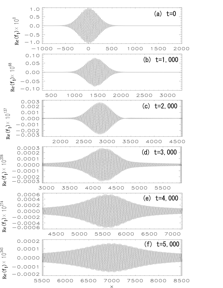
Figure 5: Imaginary time evolution of wave packet superluminal propagation in pair plasma, with $\sigma=50$, $k_{0}=0.25$, $H=4$. Here $f_{1}$ is normalized by the maximum initial value.

References

(1)
S. Koide, K. Shibata, and T. Kudoh, Astrophys. J. Lett., 495, L63 (1998).
(2)
S. Koide, K. Shibata, and T. Kudoh, Astrophys. J. , 522, 727 (1999).
(3)
S. Koide, D. L. Meier, K. Shibata, and T. Kudoh, Astrophys. J. , 536, 668 (2000).
(4)
S. Koide, K. Shibata, T. Kudoh, and D. L. Meier, Science, 295, 1688 (2002).
(5)
S. Koide, Phys. Rev. D 67, 104010 (2003).
(6)
S. Koide, Astrophys. J. Lett, 606, L45 (2004).
(7)
S. Koide, K. Shibata, and T. Kudoh, Phys. Rev. D, 74, 044005 (2006).
(8)
Y. Mizuno, S. Yamada, S. Koide, and K. Shibata,
Astrophys. J. , 606, 395 (2004).
(9)
S. S. Komissarov, Mon. Not. R. Astron. Soc., 350, 1431 (2004).
(10)
S. S. Komissarov, and J. C. McKinney, Mon. Not. R. Astron. Soc., 377, L49 (2007).
(11)
C. F. Gammie, J. C. McKinney, and G. Toth, Astrophys. J. , 589, 444 (2003).
(12)
J. C. McKinney and C. F. Gammie, Astrophys. J. , 611, 977 (2004).
(13)
J. C. McKinney, Mon. Not. R. Astron. Soc., 368, 1561 (2006).
(14)
N. Watanabe and T. Yokoyama, Astrophys. J. Lett, 647, L123 (2006).
(15)
S. S. Komissarov, Mon. Not. R. Astron. Soc. 382, 995 (2007).
(16)
H. Ardavan, Astrophys. J. , 203, 226 (1976).
(17)
E. G. Blackman, and G. B. Field, Phys. Rev. Lett. 71, 3481 (1993).
(18)
M. Gedalin, Phys. Rev. Lett. 76, 3340 (1996).
(19)
A. Melatos and D. B. Melrose, Mon. Not. R. Astron. Soc.
279, 1168 (1996).
(20)
R. Khanna, Mon. Not. R. Astron. Soc. 294, 673 (1998).
(21)
D. L. Meier, Astrophys. J. , 605, 340 (2004).
(22)
S. Weinberg, Gravitation and Cosmology
(John Wiley & Sons, New York, 1972).
(23)
C. W. Misner, K. S. Thorne, and J. A. Wheeler,
Gravitation, (W. H. Freeman and Company, New York, 1970).
(24)
P. M. Bellan, Fundamentals of Plasma Physics,
(Cambridge University Press, Cambridge, 2006).
(25)
S. Koide and K. Arai, Astrophys. J. , 682, 1124 (2008).
(26)
J. F. Wardle, D. C. Homan, R. Ojha, and D. H. Roberts,
Nature 395, 457 (1998).