Induced $p$-wave superfluidity in two dimensions:
Brane world in cold atoms and nonrelativistic defect CFTs

Abstract

We propose to use a two-species Fermi gas with the interspecies $s$-wave Feshbach resonance to realize $p$-wave superfluidity in two dimensions. By confining one species of fermions in a two-dimensional plane immersed in the background three-dimensional Fermi sea of the other species, an attractive interaction is induced between two-dimensional fermions. We compute the pairing gap in the weak-coupling regime and show that it has the symmetry of $p_{x}{+}ip_{y}$. Because the magnitude of the pairing gap increases toward the unitarity limit, it is possible that the critical temperature for the $p_{x}{+}ip_{y}$-wave superfluidity becomes within experimental reach. The resulting system has a potential application to topological quantum computation using vortices with non-Abelian statistics. We also discuss aspects of our system in the unitarity limit as a “nonrelativistic defect conformal field theory (CFT)”. The reduced Schrödinger algebra, operator-state correspondence, scaling dimensions of composite operators, and operator product expansions are investigated.

I Introduction

Experiments using ultracold atomic gases have achieved great success in realizing a new type of fermionic superfluids. By arbitrarily varying the strength of interaction via the Feshbach resonance, the weakly-interacting BCS superfluid, the strongly-interacting unitary Fermi gas, and the Bose-Einstein condensate of tightly-bound molecules have been observed and extensively studied Ketterle:2008 ; review_theory . So far, the fermionic superfluids in atomic gases have been limited to $s$-wave pairings between different spin states. Therefore the realization of $p$-wave superfluids in spin-polarized Fermi gases is a natural next goal in the cold atom community. In particular, a “weakly-paired” $p_{x}{+}ip_{y}$-wave superfluid in two dimensions is of special interest because its vortices support zero-energy Majorana fermions and exhibit non-Abelian statistics Read:2000 . As a practical application, it has been proposed to use such a system as a platform for topological quantum computation Tewari:2007 .

Most theoretical studies regarding the $p$-wave superfluids in atomic gases assume the availability of $p$-wave Feshbach resonances Tewari:2007 ; Bohn:2000 ; Ho:2005 ; Ohashi:2005 ; Gurarie:2005 ; Botelho:2005 ; Cheng:2005 ; Iskin:2006 (for alternative mechanisms, see Refs. You:1999 ; Efremov:2000 ; Efremov:2002 ; Gaudio:2005 ; Bulgac:2006gh ; Zhang:2008 ). However, experimental studies showed that the $p$-wave Feshbach molecules are unstable due to atom-molecule and molecule-molecule inelastic collisions with their lifetimes up to 20 ms Regal:2003 ; Zhang:2004 ; Schunck:2005 ; Gunter:2005 ; Gaebler:2007 ; Fuchs:2008 ; Jin:2008 ; Inada:2008 . This is in contrast to the long-lived $s$-wave Feshbach molecules where the inelastic collisions are suppressed due to the Pauli exclusion principle Petrov:2004 . Because the decay rate of the $p$-wave Feshbach molecules is comparable to the interaction energy scale, the $p$-wave superfluid without additional mechanism to suppress the inelastic collisions will not reach its equilibrium before it decays Levinsen:2007 ; Jona-Lasinio:2008 .

In this paper, we propose a novel approach to realize the $p$-wave superfluidity in two dimensions, without assuming the $p$-wave Feshbach resonance. The idea is to utilize a two-species Fermi gas (fermion atomic species $A$ and $B$) with the interspecies $s$-wave Feshbach resonance in 2D-3D mixed dimensions Nishida:2008kr . Here $A$ atoms are confined in a two-dimensional plane (2D) by means of a strong optical trap, while $B$ atoms are free from the confinement and hence in the three-dimensional space (3D). It has been shown that the interspecies short-range interaction between $A$ and $B$ atoms is characterized by a single parameter, the effective scattering length $a_{\mathrm{eff}}$, whose value is arbitrarily tunable by the interspecies $s$-wave Feshbach resonance Nishida:2008kr . The system under consideration can be set up in experiments with the use of the recently observed quantum degenerate Fermi-Fermi mixture of ${}^{6}\mathrm{Li}$ and ${}^{40}\mathrm{K}$ atoms and their interspecies $s$-wave Feshbach resonances Taglieber:2008 ; Wille:2008 .

In such a system, we will show that the background 3D Fermi sea of $B$ atoms induces an attractive interaction between $A$ atoms in 2D. Because $A$ atoms are identical fermions, the dominant pairing takes place in the $p$-wave channel. We will compute the pairing gap in the controllable weak-coupling regime and show that it has the symmetry of $p_{x}{+}ip_{y}$. Because the magnitude of the pairing gap increases toward the unitarity limit $|a_{\mathrm{eff}}|\to\infty$, the critical temperature for the $p_{x}{+}ip_{y}$-wave superfluidity is expected to become within experimental reach. As it is mentioned above, the resulting system has a potential application to topological quantum computation using vortices with non-Abelian statistics Read:2000 ; Tewari:2007 .

This paper is organized as follows. In Sec. II, we describe the two-species Fermi gas in the 2D-3D mixed dimensions. In particular, we give its field-theoretical formulation in a detailed way because such a system may not be familiar to the cold atom community. Then in Sec. III, we compute the induced interaction between two-dimensional fermions, the pairing gap, and its symmetry in the weak-coupling regime where we can perform the controlled perturbative analysis. Finally, summary and discussions are given in Sec. IV and here a very interesting analogy of the system investigated in this paper with the brane-world model of the universe is pointed out. Two additional materials are presented in Appendices. The absence of the interspecies pairing at weak coupling is shown in the Appendix A. In the Appendix B, we discuss aspects of our system in the unitarity limit as a nonrelativistic defect conformal field theory. We derive the reduced Schrödinger algebra and the operator-state correspondence in general nonrelativistic defect conformal field theories. We also study scaling dimensions of few-body composite operators and operator product expansions in our 2D-3D mixed dimensions. In particular, critical mass ratios for Efimov bound states are obtained.

II Two-species Fermi gas in 2D-3D mixed dimensions

II.1 Field theoretical formulation

The two-species Fermi gas in the 2D-3D mixed dimensions is described by the following action (here and below $\hbar=1$ and $k_{\mathrm{B}}=1$):

$$\begin{split}S&=\int\!dt\int\!d{\bm{x}}\,\psi_{A}^{\dagger}(t,{\bm{x}})\left(i\partial_{t}+\frac{\bm{\nabla}_{\!{\bm{x}}}^{2}}{2m_{A}}+\mu_{A}\right)\psi_{A}(t,{\bm{x}})\\ &\quad+\int\!dt\int\!d{\bm{x}}\!\int\!dz\,\psi_{B}^{\dagger}(t,{\bm{x}},z)\left(i\partial_{t}+\frac{\bm{\nabla}_{\!{\bm{x}}}^{2}+\nabla_{\!z}^{2}}{2m_{B}}+\mu_{B}\right)\psi_{B}(t,{\bm{x}},z)\\ &\quad+g_{0}\int\!dt\int\!d{\bm{x}}\,\psi_{A}^{\dagger}(t,{\bm{x}})\psi_{B}^{\dagger}(t,{\bm{x}},0)\psi_{B}(t,{\bm{x}},0)\psi_{A}(t,{\bm{x}}).\end{split}$$ (1)

Here ${\bm{x}}=(x,y)$ is a two-dimensional coordinate and $({\bm{x}},z)$ is a three-dimensional coordinate. $\psi_{A}(t,{\bm{x}})$ is a fermionic field describing $A$ atoms confined in a two-dimensional plane located at $z=0$ and $\psi_{B}(t,{\bm{x}},z)$ is another fermionic field describing $B$ atoms in the three-dimensional bulk space. $m_{A(B)}$ is the atomic mass of $A(B)$ atoms and the density of each species $n_{A(B)}$ is controlled by the chemical potential $\mu_{A(B)}$. The interspecies interaction is short-ranged and thus occurs only on the plane at $z=0$, while $B$ atoms can propagate into the $z$-direction (“extra dimension”) [see also Fig. 1].

$g_{0}$ is a cutoff dependent bare coupling. Because dimensions of the fields are $[\psi_{A}]=1$ and $[\psi_{B}]=\frac{3}{2}$ in units of momentum, the dimension of the coupling becomes $[g_{0}]=-1$. This implies that the theory has a linear divergence as it is well known in the usual 3D case. However, as we will see below, the linear divergence can be renormalized into $g_{0}$ and all physical observables can be expressed in terms of the physical parameter, the effective scattering length $a_{\mathrm{eff}}$. We note that interactions between the same species of fermions (without the $p$-wave Feshbach resonance) are generally weak and can be neglected at low energies.

The bare propagator of $\psi_{A}$ field is $\langle T\,\psi_{A}(t,{\bm{x}})\psi_{A}^{\dagger}(t^{\prime},{\bm{x}}^{\prime})\rangle_{0}$ where the expectation value is evaluated with the noninteracting action. Because of the translational symmetry in the plane, its Fourier transform is given by the usual form:

$$iG_{A}(p_{0},{\bm{p}})=\frac{i}{p_{0}-\frac{{\bm{p}}^{2}}{2m_{A}}+\mu_{A}+i\delta},$$ (2)

where $p_{0}$ is the frequency and ${\bm{p}}=(p_{x},p_{y})$ is the two-dimensional momentum. Similarly the bare propagator of $\psi_{B}$ field is given by $\langle T\,\psi_{B}(t,{\bm{x}},z)\psi_{B}^{\dagger}(t^{\prime},{\bm{x}}^{\prime},z^{\prime})\rangle_{0}$. We shall not perform its full Fourier transformation because once the interaction between $\psi_{A}$ and $\psi_{B}$ fields is turned on, the translational symmetry along the $z$-direction is lost. Instead it is convenient to employ the following mixed representation:

$$iG_{B}(p_{0},{\bm{p}};z-z^{\prime})=i\int\!\frac{dp_{z}}{2\pi}\frac{e^{ip_{z}(z-z^{\prime})}}{p_{0}-\frac{{\bm{p}}^{2}+p_{z}^{\,2}}{2m_{B}}+\mu_{B}+i\delta},$$ (3)

where $p_{z}$ is the momentum conjugate to $z-z^{\prime}$. We will often use the propagator where $z$ and $z^{\prime}$ are fixed on the plane; $z=z^{\prime}=0$. In such a case, we suppress the last argument in $G_{B}(p_{0},{\bm{p}};z-z^{\prime})$ and denote it simply as $G_{B}(p_{0},{\bm{p}})\equiv G_{B}(p_{0},{\bm{p}};0)$. Hereafter we shall use a shorthand notation $p=(p_{0},{\bm{p}})$.

II.2 Two-particle scattering in vacuum

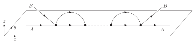
Figure 1: Two-particle scattering of $A$ and $B$ atoms. The $A$ atom is confined in a plane located at $z=0$ while the $B$ atom can propagate into the $z$-direction (“extra dimension”). The interspecies short-range interaction takes plane only on the plane.

We first study the two-particle scattering in vacuum ($\mu_{A}=\mu_{B}=0$) in order to relate the bare coupling $g_{0}$ with the effective scattering length $a_{\mathrm{eff}}$. The scattering process of $A$ and $B$ atoms is schematically depicted in Fig. 1. By summing a geometric series of Feynman diagrams, the scattering amplitude $\mathcal{A}(p)$ is written as

$$\begin{split}[i\mathcal{A}(p)]^{-1}&=\frac{1}{ig_{0}}-\int\!\frac{dk_{0}d{\bm{k}}}{(2\pi)^{3}}\,iG_{A}(p-k)\,iG_{B}(k)\\ &=\frac{1}{ig_{0}}+i\int\!\frac{d{\bm{k}}}{(2\pi)^{2}}\frac{\sqrt{\frac{m_{B}}{2}}}{\sqrt{\frac{({\bm{p}}-{\bm{k}})^{2}}{2m_{A}}+\frac{{\bm{k}}^{2}}{2m_{B}}-p_{0}-i0^{+}}}.\end{split}$$ (4)

We can see that the ${\bm{k}}$ integration is ultraviolet divergent. The usual way to regulate the integral is to introduce a momentum cutoff $|{\bm{k}}|<\Lambda_{k}$ and adjust the $\Lambda_{k}$-dependence of $g_{0}$ so that the physics does not depend on $\Lambda_{k}$. The integration over ${\bm{k}}$ leads to

$$\mathcal{A}(p)=\frac{1}{\frac{1}{g_{0}}-\frac{\sqrt{m_{B}m_{AB}}}{2\pi}\left(\Lambda_{k}-\sqrt{\frac{m_{AB}}{M}{\bm{p}}^{2}-2m_{AB}p_{0}-i0^{+}}\right)},$$ (5)

where $M=m_{A}+m_{B}$ is the total mass and $m_{AB}=\frac{m_{A}m_{B}}{m_{A}+m_{B}}$ is the reduced mass. By introducing the effective scattering length through

$$\frac{1}{g_{0}}-\frac{\sqrt{m_{B}m_{AB}}}{2\pi}\Lambda_{k}=-\frac{\sqrt{m_{B}m_{AB}}}{2\pi a_{\mathrm{eff}}},$$ (6)

the scattering amplitude becomes cutoff-independent:

$$\mathcal{A}(p)=\frac{2\pi}{\sqrt{m_{B}m_{AB}}}\frac{1}{-\frac{1}{a_{\mathrm{eff}}}+\sqrt{\frac{m_{AB}}{M}{\bm{p}}^{2}-2m_{AB}p_{0}-i0^{+}}}.$$ (7)

Now the interspecies interaction is solely characterized by the effective scattering length $a_{\mathrm{eff}}$. $a_{\mathrm{eff}}\to-0$ corresponds to the weak attraction and $a_{\mathrm{eff}}\to+0$ corresponds to the strong attraction just as in the usual 3D case. $|a_{\mathrm{eff}}|\to\infty$ corresponds to the unitarity limit where the scale-invariant interaction is achieved. In this limit, our theory (1) provides a novel type of nonrelativistic conformal field theories. Aspects of our system in the unitarity limit as a nonrelativistic conformal field theory will be elaborated in detail in the Appendix B.

When $a_{\mathrm{eff}}>0$, there exists a shallow two-body bound state composed of $A$ and $B$ atoms. Its binding energy $\varepsilon_{\mathrm{b}}$, defined to be positive, is obtained as a pole of the scattering amplitude when the external momentum ${\bm{p}}$ is zero:

$$\mathcal{A}(-\varepsilon_{\mathrm{b}},{\bm{0}})^{-1}=0\quad\Rightarrow\quad\varepsilon_{\mathrm{b}}=\frac{1}{2m_{AB}a_{\mathrm{eff}}^{\,2}}.$$ (8)

Thus our definition of $a_{\mathrm{eff}}$ in Eq. (7) coincides with that used in Ref. Nishida:2008kr . The two-body resonance $\varepsilon_{\mathrm{b}}\to 0$ occurs at infinite effective scattering length $a_{\mathrm{eff}}\to\infty$.

II.3 Effective versus bare scattering lengths

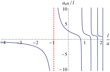
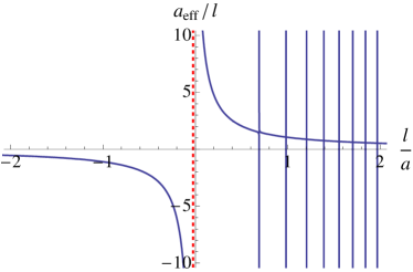
Figure 2: Effective scattering length $a_{\mathrm{eff}}/l$ as a function of the inverse bare scattering length $l/a$ for mass ratios $m_{A}/m_{B}=0.15$ (left) and $m_{A}/m_{B}=6.67$ (right) Nishida:2008kr . The vertical dotted line indicates the position of the broadest resonance.

The effective scattering length $a_{\mathrm{eff}}$ in the 2D-3D mixed dimensions depends on the bare scattering length $a$ in a free 3D space. $a$ is arbitrarily tunable by means of the interspecies $s$-wave Feshbach resonance as a function of the magnetic field applied to the system Wille:2008 . In Ref. Nishida:2008kr , the dependence of $a_{\mathrm{eff}}$ on $a$ was determined when the $A$ atom is confined by a one-dimensional harmonic potential with the oscillator frequency $\omega_{z}$. Fig. 2 shows $a_{\mathrm{eff}}/l$ plotted as a function of $l/a$ with $l\equiv\sqrt{\frac{1}{m_{A}\omega_{z}}}$ being the oscillator length Nishida:2008kr . Here the mass ratios $m_{A}/m_{B}=0.15$ and $6.67$ are chosen corresponding to the physical cases of $A={}^{6}\mathrm{Li}$, $B={}^{40}\mathrm{K}$ and $A={}^{40}\mathrm{K}$, $B={}^{6}\mathrm{Li}$, respectively.

We can see that the position of the resonance in the 2D-3D mixed dimensions ($|a_{\mathrm{eff}}|=\infty$) is shifted from the free space resonance ($|a|=\infty$) to the negative bare scattering length. It is understandable that the $AB$ bound state can be formed with a weaker attraction ($a<0$) because of the partial confinement of the $A$ atom. The broadest resonance occurs at $l/a=-0.882$ for $m_{A}/m_{B}=0.15$ and at $l/a=-0.0237$ for $m_{A}/m_{B}=6.67$. In addition to the broadest resonance, an infinite number of confinement-induced resonances appears while they are narrower Peano:2005 ; Massignan:2006 .

Using one of these resonances, the effective scattering length can be tuned to any desired value $-\infty<a_{\mathrm{eff}}^{-1}<\infty$ by simply varying $a$ or $l$. If the confinement length $l$ is much smaller than any other length scales of the system such as $a_{\mathrm{eff}}$ and mean interatomic distances at finite densities, we can neglect the motion of $A$ atoms in the confinement $z$-direction. Then the resulting system becomes the two-species Fermi gas in the 2D-3D mixture universally described by the action (1).

Ref. Nishida:2008kr also found that the many-body system near the unitarity limit $|a_{\mathrm{eff}}|\to\infty$ is stable against the formation of deep three-body bound states (Efimov effect) when the mass ratio is in the range $0.0351<m_{A}/m_{B}<6.35$ (see also the Appendix B.2). Therefore the combination of atomic species, $A={}^{6}\mathrm{Li}$ and $B={}^{40}\mathrm{K}$ ($m_{A}/m_{B}=0.15$), can be used to realize the stable 2D-3D mixed Fermi gas, while the opposite combination, $A={}^{40}\mathrm{K}$ and $B={}^{6}\mathrm{Li}$ ($m_{A}/m_{B}=6.67$), suffers the Efimov effect. However, because the mass ratio of the latter combination is just above the critical value, it may be possible that such a system becomes metastable, for example, in an optical lattice. We also note that if either $A$ or $B$ atoms are bosonic, the Efimov effect takes place for any mass ratio Nishida:2008kr . Thus for the stability of the many-body system, fermion atomic species $A$ and $B$ are essential.

II.4 Perturbation theory at finite density

In the limit of weak attraction $a_{\mathrm{eff}}\to-0$, it is straightforward to develop a perturbation theory at finite densities ($\mu_{A},\,\mu_{B}>0$). The propagator of $A$ atom is given by $iG_{A}(p)$ in Eq. (2) and the propagator of $B$ atom is given by $iG_{B}(p;z)$ in Eq. (3). From Eq. (7), we find that each interaction vertex carries a small coupling constant given by $-\frac{2\pi ia_{\mathrm{eff}}}{\sqrt{m_{B}m_{AB}}}$.

As one of applications of the perturbation theory, we compute the density distribution of $B$ atoms in the weak-coupling limit $a_{\mathrm{eff}}\to-0$. Due to the lack of translational symmetry in the $z$-direction, the density of $B$ atoms is no longer uniform. The density of $B$ atoms is given by $\tilde{n}_{B}(|z|)=\langle\psi_{B}^{\dagger}(t+0^{+},{\bm{x}},z)\psi_{B}(t,{\bm{x}},z)\rangle$, which is a function of $|z|$ because of the in-plane translational symmetry and the symmetry under $z$-parity. To the leading order in $a_{\mathrm{eff}}$, $\tilde{n}_{B}(|z|)$ is obtained as

$$\begin{split}\tilde{n}_{B}(|z|)&=-\int\!\frac{dp_{0}d{\bm{p}}}{(2\pi)^{3}}\,e^{ip_{0}0^{+}}iG_{B}(p;0)-\int\!\frac{dp_{0}d{\bm{p}}}{(2\pi)^{3}}\,iG_{B}(p;z)\left(-i\Sigma_{B}\right)iG_{B}(p;-z)\\ &=n_{B}-i\Sigma_{B}\int\!\frac{dp_{0}d{\bm{p}}dp_{z}dq_{z}}{(2\pi)^{5}}\frac{e^{ip_{z}z}}{p_{0}-\frac{{\bm{p}}^{2}+p_{z}^{\,2}}{2m_{B}}+\mu_{B}+i\delta}\frac{-e^{iq_{z}z}}{p_{0}-\frac{{\bm{p}}^{2}+q_{z}^{\,2}}{2m_{B}}+\mu_{B}+i\delta},\end{split}$$ (9)

where $n_{B}=\frac{(2m_{B}\mu_{B})^{3/2}}{6\pi^{2}}$ is the uniform density of $B$ atoms in the noninteracting limit. $\Sigma_{B}$ is a mean-field self-energy proportional to the effective scattering length $a_{\mathrm{eff}}$ and the density of $A$ atoms $n_{A}=\frac{(2m_{A}\mu_{A})}{4\pi}$:

$$\Sigma_{B}=-\frac{2\pi a_{\mathrm{eff}}}{\sqrt{m_{B}m_{AB}}}\int\!\frac{dp_{0}d{\bm{p}}}{(2\pi)^{3}}\,e^{ip_{0}0^{+}}iG_{A}(p)=\frac{2\pi a_{\mathrm{eff}}}{\sqrt{m_{B}m_{AB}}}n_{A}<0.$$ (10)

We note that the dimensions of $n_{A}$ and $n_{B}$ are different because $n_{A}$ is the two-dimensional density while $n_{B}$ is the three-dimensional density. The Fermi momentum of each species is defined through its density by $k_{\mathrm{F}\!A}\equiv\left(4\pi n_{A}\right)^{1/2}$ and $k_{\mathrm{F}\!B}\equiv\left(6\pi^{2}n_{B}\right)^{1/3}$.

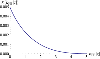
Figure 3: $\kappa(k_{\mathrm{F}\!B}|z|)$ appearing in the density distribution of $B$ atoms in Eq. (11). At $z=0$, we have $\kappa(0)=1/(64\pi)$.

The integration over $p_{0}$ in Eq. (9) results in the following expression for the density distribution:

$$\tilde{n}_{B}(|z|)=n_{B}+|a_{\mathrm{eff}}|k_{\mathrm{F}\!A}^{\,2}k_{\mathrm{F}\!B}^{\,2}\sqrt{\frac{m_{B}}{m_{AB}}}\,\kappa(k_{\mathrm{F}\!B}|z|),$$ (11)

where $\kappa(r)$ is a positive function given by

$$\kappa(r)\equiv\int_{0}^{1}\!\frac{dp\,p}{2\pi}\int_{\sqrt{1-p^{2}}}^{\infty}\!\frac{dp_{z}}{2\pi}\int_{0}^{\sqrt{1-p^{2}}}\!\frac{dq_{z}}{2\pi}\frac{2\cos[(p_{z}-q_{z})r]}{p_{z}^{\,2}-q_{z}^{\,2}}.$$ (12)

$\kappa(k_{\mathrm{F}\!B}|z|)$ is plotted in Fig. 3 and monotonously decreases as a function of $k_{\mathrm{F}\!B}|z|$. We can understand that $B$ atoms are attracted to the 2D plane at $z=0$ because of their attractive interaction with $A$ atoms confined in the plane. The density of $B$ atoms away from the 2D plane approaches that in the noninteracting limit; $\tilde{n}_{B}(|z|\to\infty)\to n_{B}$ because the interaction is suppressed there.

III Induced interaction and $p$-wave pairing in two dimensions

III.1 Induced interaction at weak coupling

Using the perturbation theory in the weak-coupling limit $a_{\mathrm{eff}}\to-0$, we now determine the interaction between two $A$ atoms in 2D induced by the existence of the 3D Fermi sea of $B$ atoms. Because we are interested in the intra-species pairing of $A$ atoms, we consider their back-to-back scattering. To the leading order in $a_{\mathrm{eff}}$, the induced interaction between $A$ atoms $V_{\mathrm{ind}}$ is described by the Feynman diagram depicted in Fig. 4 Bulgac:2006gh , which is written as

$$-\frac{i}{2}V_{\mathrm{ind}}(p,q)=-\frac{1}{2}\left(\frac{-2\pi ia_{\mathrm{eff}}}{\sqrt{m_{B}m_{AB}}}\right)^{2}\int\!\frac{dk_{0}d{\bm{k}}}{(2\pi)^{3}}\,iG_{B}(k+p-q)\,iG_{B}(k).$$ (13)

The integration over $k_{0}$ leads to

$$\begin{split}V_{\mathrm{ind}}(p,q)&=-\frac{\left(2\pi a_{\mathrm{eff}}\right)^{2}}{m_{B}m_{AB}}\int\!\frac{d{\bm{k}}dk_{z}dk^{\prime}_{z}}{(2\pi)^{4}}\\ &\quad\times\left[\frac{\theta\!\left(\frac{({\bm{k}}+{\bm{p}}-{\bm{q}})^{2}+k_{z}^{\,2}}{2m_{B}}-\mu_{B}\right)\theta\!\left(\mu_{B}-\frac{{\bm{k}}^{2}+k_{z}^{\prime 2}}{2m_{B}}\right)}{\frac{({\bm{k}}+{\bm{p}}-{\bm{q}})^{2}+k_{z}^{\,2}}{2m_{B}}-\frac{{\bm{k}}^{2}+k_{z}^{\prime 2}}{2m_{B}}-p_{0}+q_{0}-i0^{+}}+\frac{\theta\!\left(\mu_{B}-\frac{({\bm{k}}+{\bm{p}}-{\bm{q}})^{2}+k_{z}^{\,2}}{2m_{B}}\right)\theta\!\left(\frac{{\bm{k}}^{2}+k_{z}^{\prime 2}}{2m_{B}}-\mu_{B}\right)}{\frac{{\bm{k}}^{2}+k_{z}^{\prime 2}}{2m_{B}}-\frac{({\bm{k}}+{\bm{p}}-{\bm{q}})^{2}+k_{z}^{\,2}}{2m_{B}}+p_{0}-q_{0}-i0^{+}}\right].\end{split}$$ (14)

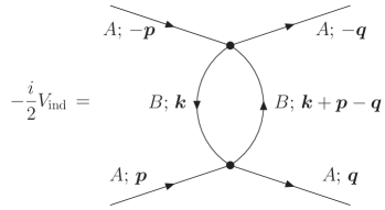
Figure 4: Interaction between two $A$ atoms in 2D induced by the 3D Fermi sea of $B$ atoms.

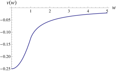
Figure 5: $v(w)$ appearing in the induced interaction in Eq. (15).

For the gap equation at weak coupling, we will need the induced interaction in which both incoming and outgoing momenta are on the 2D Fermi surface $|{\bm{p}}|=|{\bm{q}}|=k_{\mathrm{F}\!A}$, and hence, $p_{0}=q_{0}=0$. In such a static limit, we can perform the remaining integrations analytically and obtain

$$V_{\mathrm{ind}}({\bm{p}},{\bm{q}})=\frac{2\pi a_{\mathrm{eff}}^{\,2}k_{\mathrm{F}\!B}^{\,2}}{m_{AB}}\,v\!\left(\frac{|{\bm{p}}-{\bm{q}}|}{2k_{\mathrm{F}\!B}}\right),$$ (15)

where $v(w)$ is a continuous function given by

$$v(w)\equiv\begin{cases}\displaystyle-\frac{2-w^{2}}{8}&w<1\vskip 6.0pt plus 2.0pt minus 2.0pt\\ \displaystyle-\frac{\sqrt{w^{2}-1}+\left(2-w^{2}\right)\arcsin w^{-1}}{4\pi}&w>1.\end{cases}$$ (16)

The nonanalyticity of $v(w)$ at $w=1$ is due to the sharp Fermi surface of $B$ atoms. The function $v(w)$ is plotted in Fig. 5 and is negative everywhere indicating that the induced interaction between $A$ atoms is attractive. Thus an intra-species pairing in the two-dimensional plane is expected to occur. Because $A$ atoms are identical fermions, the dominant pairing takes place in the $p$-wave channel, as we will see below.

At this point, we should point out that the interspecies pairing between $A$ and $B$ atoms is unlikely in our system (except deep in the BEC regime $a_{\mathrm{eff}}\to+0$) because they live in different spatial dimensions. $B$ atoms can always escape from the 2D plane in which $A$ atoms are confined into the $z$-direction (“extra dimension”) and there the interspecies interaction is turned off. Actually, as we will show in the Appendix A, the absence of the interspecies pairing can be confirmed at weak coupling $a_{\mathrm{eff}}\to-0$. Hereafter $B$ atoms are treated as a background to induce the attraction between $A$ atoms and we investigate the intra-species pairing of $A$ atoms in 2D.

III.2 Gap equation

Once the induced interaction between $A$ atoms $V_{\mathrm{ind}}({\bm{p}},{\bm{q}})$ is obtained, the pairing of $A$ atoms in 2D is described by the BCS-type Hamiltonian:

$$\begin{split}H_{A}&=\int\!\frac{d{\bm{p}}}{(2\pi)^{2}}\left(\frac{{\bm{p}}^{2}}{2m_{A}}-\mu_{A}\right)\tilde{\psi}_{A}^{\dagger}({\bm{p}})\tilde{\psi}_{A}({\bm{p}})\\ &\quad+\frac{1}{2}\int\frac{d{\bm{k}}d{\bm{p}}d{\bm{q}}}{(2\pi)^{6}}\,\tilde{\psi}_{A}^{\dagger}\!\left(\frac{{\bm{k}}}{2}+{\bm{q}}\right)\tilde{\psi}_{A}^{\dagger}\!\left(\frac{{\bm{k}}}{2}-{\bm{q}}\right)V_{\mathrm{ind}}({\bm{p}},{\bm{q}})\,\tilde{\psi}_{A}\!\left(\frac{{\bm{k}}}{2}-{\bm{p}}\right)\tilde{\psi}_{A}\!\left(\frac{{\bm{k}}}{2}+{\bm{p}}\right),\end{split}$$ (17)

where $\tilde{\psi}_{A}({\bm{p}})$ is the Fourier transform of $\psi_{A}({\bm{x}})$. We note the property $V_{\mathrm{ind}}({\bm{p}},{\bm{q}})=V_{\mathrm{ind}}({\bm{q}},{\bm{p}})$. The pairing gap of $A$ atoms $\Delta_{\bm{p}}$ is defined to be

$$(2\pi)^{2}\delta({\bm{k}})\Delta_{\bm{p}}=\int\!\frac{d{\bm{q}}}{(2\pi)^{2}}V_{\mathrm{ind}}({\bm{p}},{\bm{q}})\left\langle\tilde{\psi}_{A}\!\left(\frac{{\bm{k}}}{2}-{\bm{q}}\right)\tilde{\psi}_{A}\!\left(\frac{{\bm{k}}}{2}+{\bm{q}}\right)\right\rangle.$$ (18)

Because of the Fermi statistics of $A$ atoms, the pairing gap has to have an odd parity; $\Delta_{-{\bm{p}}}=-\Delta_{{\bm{p}}}$. The standard mean-field calculation leads to the following self-consistent gap equation:

$$\Delta_{\bm{p}}=-\int\!\frac{d{\bm{q}}}{(2\pi)^{2}}V_{\mathrm{ind}}({\bm{p}},{\bm{q}})\frac{\Delta_{\bm{q}}}{2E_{\bm{q}}}\left[1-2n_{\mathrm{F}}(E_{\bm{q}})\right].$$ (19)

Here $E_{\bm{p}}=\sqrt{\left(\frac{{\bm{p}}^{2}}{2m_{A}}-\mu_{A}\right)^{2}+|\Delta_{\bm{p}}|^{2}}$ is the quasiparticle energy and $n_{\mathrm{F}}(E_{\bm{p}})=1/\left(e^{E_{\bm{p}}/T}+1\right)$ is the Fermi-Dirac distribution function at temperature $T$.

The gap equation (19) is a nonlinear integral equation in terms of the pairing gap $\Delta_{\bm{p}}$. However, it becomes a linear integral equation near the critical temperature $T\to T_{\mathrm{c}}$ because one can set $\Delta_{\bm{p}}\to 0$ in $E_{\bm{p}}$. In such a case, $\Delta_{\bm{p}}=e^{il\theta_{\hat{\bm{p}}}}\Delta^{(l)}$ with an odd integer $l$ being the orbital angular momentum solves the gap equation and the critical temperature $T_{\mathrm{c}}$ is determined by the equation

$$1=-N_{A}V_{\mathrm{ind}}^{(l)}\int_{0}^{\Lambda_{\varepsilon}}\!\frac{d\varepsilon}{\varepsilon}\tanh\!\left(\frac{\varepsilon}{2T_{\mathrm{c}}^{(l)}}\right).$$ (20)

Here $\Lambda_{\varepsilon}$ is an energy cutoff and $N_{A}\equiv\frac{m_{A}}{2\pi}$ is the density of states of $A$ atoms at the Fermi surface. $V_{\mathrm{ind}}^{(l)}=V_{\mathrm{ind}}^{(-l)}$ is the partial-wave projection of the induced interaction given by

$$V_{\mathrm{ind}}^{(l)}=\frac{2\pi a_{\mathrm{eff}}^{\,2}k_{\mathrm{F}\!B}^{\,2}}{m_{AB}}\int_{0}^{\pi}\!\frac{d\theta}{\pi}\cos(l\theta)\,v\!\left(\frac{k_{\mathrm{F}\!A}}{k_{\mathrm{F}\!B}}\sqrt{\frac{1-\cos\theta}{2}}\right)\equiv\frac{2\pi a_{\mathrm{eff}}^{\,2}k_{\mathrm{F}\!B}^{\,2}}{m_{AB}}\,v^{(l)}\!\left(\frac{k_{\mathrm{F}\!A}}{k_{\mathrm{F}\!B}}\right).$$ (21)

When the projected interaction is attractive $N_{A}V_{\mathrm{ind}}^{(l)}<0$, it is easy to solve Eq. (20) and we find

$$\frac{T_{\mathrm{c}}^{(l)}}{\varepsilon_{\mathrm{F}\!A}}\sim\exp\!\left(\frac{1}{N_{A}V_{\mathrm{ind}}^{(l)}}\right),$$ (22)

where the energy cutoff is chosen to be the order of the Fermi energy of $A$ atoms; $\Lambda_{\varepsilon}\sim\varepsilon_{\mathrm{F}\!A}=\frac{k_{\mathrm{F}\!A}^{\,2}}{2m_{A}}$. Because one can confirm that the induced attraction (21) is strongest in the $p$-wave channel, we have the highest critical temperature for $|l|=1$; $T_{\mathrm{c}}^{(1)}\gg T_{\mathrm{c}}^{(|l|\geq 3)}$. Therefore we can neglect the coupling between different partial waves and concentrate on $p$-wave pairings.

III.3 Pairing gap and its symmetry

We now solve the gap equation for the $p$-wave pairing at zero temperature $T=0$. We parameterize the angle dependence of the pairing gap as $\Delta_{\bm{p}}=f(\theta_{\hat{\bm{p}}})\Delta_{f}$, where ${\bm{p}}=k_{\mathrm{F}\!A}(\cos\theta_{\hat{{\bm{p}}}},\sin\theta_{\hat{{\bm{p}}}})$ and $f(\theta_{\hat{\bm{p}}})=b_{+}e^{i\theta_{\hat{\bm{p}}}}+b_{-}e^{-i\theta_{\hat{\bm{p}}}}$ with $|b_{+}|^{2}+|b_{-}|^{2}=1$. For example, $b_{+}=1$ and $b_{-}=0$ corresponds to a $p_{x}{+}ip_{y}$-wave pairing and $b_{+}=b_{-}=1/\sqrt{2}$ corresponds to a $p_{x}$-wave pairing. Substituting $\Delta_{\bm{p}}=f(\theta_{\hat{\bm{p}}})\Delta_{f}$ into the gap equation (19) at $T=0$, we obtain

$$\begin{split}1&=-N_{A}V_{\mathrm{ind}}^{(1)}\int_{0}^{\Lambda_{\varepsilon}}\!d\varepsilon\int_{0}^{2\pi}\!\frac{d\theta_{\hat{\bm{q}}}}{2\pi}\frac{|f(\theta_{\hat{\bm{q}}})|^{2}}{\sqrt{\varepsilon^{2}+|f(\theta_{\hat{\bm{q}}})\Delta_{f}|^{2}}}\\ &\simeq-N_{A}V_{\mathrm{ind}}^{(1)}\int_{0}^{2\pi}\!\frac{d\theta_{\hat{\bm{q}}}}{2\pi}|f(\theta_{\hat{\bm{q}}})|^{2}\ln\!\left(\frac{2\Lambda_{\varepsilon}}{|f(\theta_{\hat{\bm{q}}})\Delta_{f}|}\right).\end{split}$$ (23)

Thus we find that the modulus of the pairing gap is given by

$$\frac{|\Delta_{f}|}{\varepsilon_{\mathrm{F}\!A}}\sim\exp\!\left(\frac{1}{N_{A}V_{\mathrm{ind}}^{(1)}}-\int_{0}^{2\pi}\!\frac{d\theta}{2\pi}|f(\theta)|^{2}\ln|f(\theta)|\right).$$ (24)

The angle dependence of the pairing gap $f(\theta)$ is determined so that the ground state energy is minimized Anderson:1961 . Because the gain of energy density due to the condensation is given by

$$\langle\mathcal{H}_{A}\rangle-\langle\mathcal{H}_{A}\rangle\bigr{|}_{|\Delta_{f}|=0}=-\frac{N_{A}}{4}|\Delta_{f}|^{2},$$ (25)

the ground state energy is minimized when $|\Delta_{f}|$ is maximized. From Eq. (24), we can show that the maximum $|\Delta_{f}|$ is achieved when $f(\theta)=e^{\pm i\theta}$ corresponding to the $p_{x}{\pm}ip_{y}$-wave pairing. Therefore the pairing gap realized in our system becomes

$$\frac{\Delta_{\bm{p}}}{\varepsilon_{\mathrm{F}\!A}}\sim e^{\pm i\theta_{\hat{\bm{p}}}}\exp\!\left(\frac{1}{N_{A}V_{\mathrm{ind}}^{(1)}}\right).$$ (26)

We note that the pairing symmetry $p_{x}{\pm}ip_{y}$ is favored because of the isotropy of the induced interaction; $V_{\mathrm{ind}}^{(1)}=V_{\mathrm{ind}}^{(-1)}$. This is in contrast to the $p$-wave Feshbach resonance where the interatomic interaction can be anisotropic due to the magnetic dipole-dipole interaction Ticknor:2004 . In such a case, some parameter-tunings are necessary to realize the $p_{x}{\pm}ip_{y}$-wave pairing Gurarie:2005 ; Cheng:2005 .

III.4 Optimizing the pairing gap

In order for the experimental realization of the proposed $p_{x}{+}ip_{y}$-wave superfluidity, the critical temperature (22) and the magnitude of the pairing gap (26) have to be large enough. Thus we look for a condition in which $T_{\mathrm{c}}^{(1)}\sim|\Delta_{\bm{p}}|\sim\varepsilon_{\mathrm{F}\!A}\exp\!\left[1/\left(N_{A}V_{\mathrm{ind}}^{(1)}\right)\right]$ is maximized. From Eq. (21), $N_{A}V_{\mathrm{ind}}^{(1)}$ is given by

$$N_{A}V_{\mathrm{ind}}^{(1)}=\frac{m_{A}a_{\mathrm{eff}}^{\,2}k_{\mathrm{F}\!B}^{\,2}}{m_{AB}}\,v^{(1)}\!\left(\frac{k_{\mathrm{F}\!A}}{k_{\mathrm{F}\!B}}\right)$$ (27)

with the negative function $v^{(1)}(k_{\mathrm{F}\!A}/k_{\mathrm{F}\!B})$ plotted in Fig. 6. Because the induced interaction in the $p$-wave channel is attractive $N_{A}V_{\mathrm{ind}}^{(1)}<0$, one would like to minimize $N_{A}V_{\mathrm{ind}}^{(1)}$.

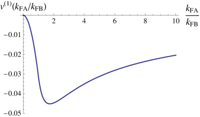
Figure 6: $v^{(1)}(k_{\mathrm{F}\!A}/k_{\mathrm{F}\!B})$ appearing in the $p$-wave projection of the induced interaction in Eq. (21).

One possible way to optimize the pairing gap is to control the densities of $A$ and $B$ atoms Bulgac:2006gh . Because our perturbative calculation relies on the smallness of $|a_{\mathrm{eff}}k_{\mathrm{F}\!B}|$, we fix $a_{\mathrm{eff}}k_{\mathrm{F}\!B}$ and vary the ratio in the two Fermi momenta $k_{\mathrm{F}\!A}/k_{\mathrm{F}\!B}$. We find that the function $v^{(1)}(k_{\mathrm{F}\!A}/k_{\mathrm{F}\!B})$ has an minimum $v^{(1)}=-0.0452$ at $k_{\mathrm{F}\!A}/k_{\mathrm{F}\!B}=1.75$ (see Fig. 6). Thus, within our perturbative calculation, the maximum pairing gap becomes

$$\frac{\Delta_{\bm{p}}^{\mathrm{max}}}{\varepsilon_{\mathrm{F}\!A}}\sim e^{\pm i\theta_{\hat{\bm{p}}}}\exp\!\left(-\frac{22.1\,m_{AB}}{m_{A}a_{\mathrm{eff}}^{\,2}k_{\mathrm{F}\!B}^{\,2}}\right).$$ (28)

The pairing gap can be further enhanced by changing the mass ratio $m_{A}/m_{B}$. Because of the factor $m_{AB}/m_{A}$ in the exponent, the larger mass of $A$ atoms in 2D increases the pairing gap. For example, the combination of atomic species $A={}^{40}\mathrm{K}$ and $B={}^{6}\mathrm{Li}$ has $m_{A}/m_{B}=6.67$, and hence, the pairing gap becomes

$$\frac{\Delta_{\bm{p}}^{\mathrm{Max}}}{\varepsilon_{\mathrm{F}\!A}}\sim e^{\pm i\theta_{\hat{\bm{p}}}}\exp\!\left(-\frac{3.29}{a_{\mathrm{eff}}^{\,2}k_{\mathrm{F}\!B}^{\,2}}\right).$$ (29)

Now the exponential factor is not hopelessly small. If one could extrapolate our perturbative result to $|a_{\mathrm{eff}}k_{\mathrm{F}\!B}|\approx 1$, we would have $\exp\!\left(-\frac{3.29}{a_{\mathrm{eff}}^{\,2}k_{\mathrm{F}\!B}^{\,2}}\right)\approx 0.04$. Furthermore, in the unitarity limit $|a_{\mathrm{eff}}|\to\infty$, the pairing gap is expected to be the same order as the Fermi energy; $\Delta_{\bm{p}}\sim e^{\pm i\theta_{\hat{\bm{p}}}}\varepsilon_{\mathrm{F}\!A}$. Therefore it is possible that the critical temperature for the $p_{x}{+}ip_{y}$-wave superfluidity becomes within experimental reach, in particular, near the unitarity limit.

III.5 Nonperturbative approaches near the unitarity limit

So far, we have performed the controlled perturbative analysis in the weak-coupling regime $a_{\mathrm{eff}}\to-0$. An important quantitative question is how high the critical temperature $T_{\mathrm{c}}^{(1)}$ can be near the unitarity limit $|a_{\mathrm{eff}}|\to\infty$. Ideally one would like to answer this question by employing quantum Monte Carlo simulations while they will suffer fermion sign problems because of the intrinsic asymmetry between $A$ and $B$ atoms in our 2D-3D mixture. Instead it is possible to estimate $T_{\mathrm{c}}^{(1)}$ by using nonperturbative analytical methods such as the $\epsilon$ expansion Nishida:2006br ; Nishida:2006eu ; Nishida:2006rp ; Nishida:2006wk and the $1/N$ expansion Nikolic:2007 ; Veillette:2007 .

The application of the $1/N$ expansion technique to our 2D-3D mixture is straightforward. We generalize the two-species Fermi gas in Eq. (1) to a $(2N)$-species Fermi gas in which $N$ species live in 2D while the other $N$ species live in 3D. The interaction among them occurs on the 2D plane and is assumed to be the $\mathrm{Sp}(2N)$-symmetric form Nikolic:2007 ; Veillette:2007 . Then we utilize the small parameter $1/N\ll 1$ to perform systematic expansions.

Here we comment on the application of the $\epsilon$ expansion technique to mixed-dimensional systems. Suppose $A$ and $B$ atoms live in $d_{A}$- and $d_{B}$-dimensional spaces, respectively, where the former space is a subset of the latter space with $d_{A}\leq d_{B}$. Such a system is described by the action analogous to Eq. (1). Now the dimensions of the fields change to $[\psi_{A}]=d_{A}/2$ and $[\psi_{B}]=d_{B}/2$ in units of momentum, and thus, the dimension of the coupling becomes $[g_{0}]=2-d_{B}$. As far as $[g_{0}]>-2$ is satisfied, the theory is renormalizable Nishida:2006eu . We note that $[g_{0}]$ depends only on the bulk spatial dimension $d_{B}$ indicating that $d_{B}$ plays a central role in the $\epsilon$ expansion. In the general combination of the spatial dimensions, one can study the two-particle scattering in vacuum as it was done in Sec. II.2. Using the dimensional regularization, the scattering amplitude $\mathcal{A}(p)$ at the scale-invariant unitarity point is found to be

$$\mathcal{A}(p)=-\frac{\left(\frac{m_{B}}{m_{AB}}\right)^{d_{A}/2}\left(\frac{2\pi}{m_{B}}\right)^{d_{B}/2}}{\Gamma\!\left(1-\frac{d_{B}}{2}\right)\left(\frac{{\bm{p}}^{2}}{2M}-p_{0}-i0^{+}\right)^{d_{B}/2-1}},$$ (30)

where ${\bm{p}}$ is the $d_{A}$-dimensional momentum. We can see that the scattering amplitude vanishes in the limits of $d_{B}\to 4$ and $d_{B}\to 2$ indicating that these two spacial dimensions correspond to noninteracting limits. Accordingly we can develop systematic expansions in terms of $\epsilon=4-d_{B}\ll 1$ and $\bar{\epsilon}=d_{B}-2\ll 1$ around those special dimensions Nishida:2006br ; Nishida:2006eu ; Nishida:2006rp ; Nishida:2006wk . We note that the other spatial dimension $d_{A}(\leq d_{B})$ is arbitrary in this approach.

The estimation of $T_{\mathrm{c}}^{(1)}$ near the unitarity limit using the above nonperturbative approaches will be left for future works.

IV Summary and discussions

In this paper, we presented theoretical prospects to realize the $p$-wave superfluidity in two dimensions by using a two-species Fermi gas (fermion atomic species $A$ and $B$) with the interspecies $s$-wave Feshbach resonance. By confining $A$ atoms in a 2D plane immersed in the background 3D Fermi sea of $B$ atoms, an attractive interaction is induced between $A$ atoms. Because $A$ atoms are identical fermions, the dominant pairing takes place in the $p$-wave channel. In the weak-coupling regime $a_{\mathrm{eff}}\to-0$ where the controlled perturbative analysis is available in terms of the effective scattering length, we computed the pairing gap and showed that it has the symmetry of $p_{x}{+}ip_{y}$. Because the magnitude of the pairing gap increases toward the unitarity limit $|a_{\mathrm{eff}}|\to\infty$, the critical temperature for the $p_{x}{+}ip_{y}$-wave superfluidity is expected to become within experimental reach. As it is mentioned in the Introduction, the resulting system has a potential application to topological quantum computation using vortices with non-Abelian statistics Read:2000 ; Tewari:2007 .

Figure 7: Proposed phase diagram of a two-species Fermi gas in the 2D-3D mixture as a function of the inverse effective scattering length $(a_{\mathrm{eff}}k_{\mathrm{F}\!A})^{-1}$ at zero temperature. There is a quantum phase transition at $(a_{\mathrm{eff}}k_{\mathrm{F}\!A})^{-1}\simeq O(1)$ from the 2D-3D mixed Fermi gas with the 2D $p_{x}{+}ip_{y}$-wave superfluidity (2D $p$-SF) to the 2D Bose-Einstein condensation of localized $s$-wave molecules (2D BEC).

It is worthwhile to clarify what happens deep in the BEC regime $a_{\mathrm{eff}}\to+0$ in our 2D-3D mixture. In this limit, $A$ atoms in 2D capture $B$ atoms to form tightly-bound molecules and the resulting system consists of the molecules localized on the 2D plane plus excess $A$ or $B$ atoms. When the size of the molecules $\sim a_{\mathrm{eff}}$ becomes smaller than the mean interatomic distance in 2D $\sim k_{\mathrm{F}\!A}^{-1}$, the molecules behave as two-dimensional bosons and therefore the ground state will be a 2D Bose-Einstein condensate of the $s$-wave molecules. Consequently, there has to be a quantum phase transition from the 2D-3D mixed Fermi gas with the 2D $p_{x}{+}ip_{y}$-wave pairing [$-\infty<(a_{\mathrm{eff}}k_{\mathrm{F}\!A})^{-1}\lesssim O(1)$] to the 2D Bose-Einstein condensation of the $s$-wave molecules [$O(1)\lesssim(a_{\mathrm{eff}}k_{\mathrm{F}\!A})^{-1}<+\infty$]. The proposed phase diagram as a function of the inverse effective scattering length is shown in Fig. 7. These two phases can be distinguished by radio-frequency spectroscopy experiments. In the 2D-3D mixed Fermi gas with the 2D $p_{x}{+}ip_{y}$-wave pairing, $A$ atoms are fully gapped while $B$ atoms remain gapless. On the other hand, in the 2D Bose-Einstein condensation of the $s$-wave molecules, both $A$ and $B$ atoms are fully gapped.

Readers may wonder why we did not consider a system in which both $A$ and $B$ atoms are confined in a two-dimensional plane to realize the induced $p$-wave superfluidity in 2D. In this case, $A$ and $B$ atoms always form bound molecules in 2D and thus the ground state of the system tends to be an $s$-wave paired state. In order to break the interspecies $s$-wave pairing, one needs to weaken the interspecies attraction with a large density imbalance introduced He:2008 . This would be a disadvantage in order to achieve a high critical temperature for the $p$-wave superfluidity in 2D.

A remarkable aspect of our two-species fermions in the 2D-3D mixed dimensions is that the system in the unitarity limit $|a_{\mathrm{eff}}|\to\infty$ is described by a nonrelativistic defect conformal field theory, which is a novel class of quantum field theories that has not been paid attention to so far. We elaborated this aspect in detail in the Appendix B.

Finally, it is very interesting to point out the analogy of the system investigated in this paper with the brane-world model of the universe. In the brane-world scenario, the ordinary matter is considered to be confined in a three-dimensional space (brane) embedded in higher dimensions (bulk) where gravitons can propagate Maartens:2003tw . The gravitational force between matters is induced by the exchange of the graviton. Similarly, in our system, the interaction between $A$ atoms confined in the 2D plane (“2D brane”) is induced by the exchange of $B$ atoms in higher dimensions (“3D bulk”). Within this fascinating analogy, our two-species Fermi gas in the 2D-3D mixed dimensions can be regarded as a brane world in cold atoms!

Acknowledgments

This work was motivated by the previous study Nishida:2008kr performed in collaboration with S. Tan to whom the author is grateful. The author also thanks D. T. Son for introducing a notion of defect conformal field theories to him. This work was supported in part by JSPS Postdoctoral Fellowship for Research Abroad and MIT Pappalardo Fellowship in Physics.

Appendix A Absence of interspecies pairing at weak coupling

Here we show the absence of the interspecies pairing between $A$ and $B$ atoms in the 2D-3D mixed dimensions in the weak-coupling regime $a_{\mathrm{eff}}\to-0$. We consider the Nambu-Gor’kov-type propagator in the $2\times 2$ matrix form:

$$i\mathcal{G}(t-t^{\prime},{\bm{x}}-{\bm{x}}^{\prime})=\begin{pmatrix}\langle T\,\psi_{A}(t,{\bm{x}})\psi_{A}^{\dagger}(t^{\prime},{\bm{x}}^{\prime})\rangle&\langle T\,\psi_{A}(t,{\bm{x}})\psi_{B}(t^{\prime},{\bm{x}}^{\prime},0)\rangle\\ \langle T\,\psi_{B}^{\dagger}(t,{\bm{x}},0)\psi_{A}^{\dagger}(t^{\prime},{\bm{x}}^{\prime})\rangle&\langle T\,\psi_{B}^{\dagger}(t,{\bm{x}},0)\psi_{B}(t^{\prime},{\bm{x}}^{\prime},0)\rangle\end{pmatrix}.$$ (31)

In the mean-field approximation, the above propagator in the momentum space becomes

$$\tilde{\mathcal{G}}(p)=\begin{pmatrix}\frac{G_{B}^{-1}(-p)}{G_{A}^{-1}(p)G_{B}^{-1}(-p)+|\phi_{0}|^{2}}&\frac{\phi_{0}}{G_{A}^{-1}(p)G_{B}^{-1}(-p)+|\phi_{0}|^{2}}\\ \frac{\phi_{0}^{*}}{G_{A}^{-1}(p)G_{B}^{-1}(-p)+|\phi_{0}|^{2}}&\frac{-G_{A}^{-1}(p)}{G_{A}^{-1}(p)G_{B}^{-1}(-p)+|\phi_{0}|^{2}}\end{pmatrix},$$ (32)

where $\phi_{0}=\langle g_{0}\,\psi_{B}(t,{\bm{x}},0)\psi_{A}(t,{\bm{x}})\rangle$ is a condensate determined by the self-consistent gap equation:

$$\begin{split}\frac{\phi_{0}}{g_{0}}&=-i\int\!\frac{dp_{0}d{\bm{p}}}{(2\pi)^{3}}\,\tilde{\mathcal{G}}_{12}(p)\\ &=-\sqrt{\frac{m_{B}}{2}}\int\!\frac{dp_{0}d{\bm{p}}}{(2\pi)^{3}}\frac{\phi_{0}}{\left(ip_{0}-\frac{{\bm{p}}^{2}}{2m_{A}}+\mu_{A}\right)\sqrt{ip_{0}+\frac{{\bm{p}}^{2}}{2m_{B}}-\mu_{B}}-\sqrt{\frac{m_{B}}{2}}|\phi_{0}|^{2}}.\end{split}$$ (33)

In the last line, we analytically continued $p_{0}$ to the imaginary frequency; $p_{0}\to ip_{0}$. Introducing the effective scattering length via Eq. (6), we obtain the following renormalized gap equation:

$$-\frac{\sqrt{2m_{AB}}}{2\pi a_{\mathrm{eff}}}=\int\!\frac{dp_{0}d{\bm{p}}}{(2\pi)^{3}}\left[\frac{1}{\left(ip_{0}-\frac{{\bm{p}}^{2}}{2m_{A}}\right)\sqrt{ip_{0}+\frac{{\bm{p}}^{2}}{2m_{B}}}}-\frac{1}{\left(ip_{0}-\frac{{\bm{p}}^{2}}{2m_{A}}+\mu_{A}\right)\sqrt{ip_{0}+\frac{{\bm{p}}^{2}}{2m_{B}}-\mu_{B}}-\sqrt{\frac{m_{B}}{2}}|\phi_{0}|^{2}}\right].$$ (34)

For simplicity, we shall consider the equal masses $m_{A}=m_{B}=m$ and equal chemical potentials $\mu_{A}=\mu_{B}=\mu$ where the interspecies pairing is guaranteed in the usual 3D case. However, in the 2D-3D mixture, we can see that the right-hand side of Eq. (34) does not have any singularity around the Fermi surface, $p_{0}\sim 0$ and $\frac{{\bm{p}}^{2}}{2m}\sim\mu$, in the limit $|\phi_{0}|\to 0$, and hence, the integral is bounded from above. This can be understood as an absence of the Cooper instability because of the intrinsic “mismatch” between the 2D and 3D Fermi surfaces. Therefore in the weak-coupling regime $a_{\mathrm{eff}}\to-0$, the gap equation (34) does not have a nontrivial solution showing that there is no interspecies pairing between $A$ and $B$ atoms.

Appendix B Aspects as a nonrelativistic defect conformal field theory

As we mentioned in Sec. II.2, two-species fermions in the 2D-3D mixed dimensions in the unitarity limit $|a_{\mathrm{eff}}|\to\infty$ (at zero density and zero temperature) provide a novel type of nonrelativistic conformal field theories (CFTs) . In this system, the three-dimensional translational, rotational, and Galilean symmetries in the bulk space are broken to the two-dimensional symmetries while scale and conformal invariance are preserved. Regarding the two-dimensional plane as a defect in the three-dimensional bulk space, our system can be thought of a nonrelativistic counterpart of defect/boundary CFTs Cardy:1984bb ; McAvity:1995zd . In Ref. Nishida:2008kr , more classes of nonrelativistic defect CFTs with zero-range and few-body resonant interactions have been proposed and are summarized in Table 1. Here we discuss aspects of our system as a nonrelativistic defect CFT (abbreviated as NRdCFT). First we derive the reduced Schrödinger algebra and the operator-state correspondence in general nonrelativistic defect CFTs. Then we study scaling dimensions of few-body composite operators and operator product expansions in our 2D-3D mixture. In particular, the critical mass ratios for the Efimov effect are obtained.

Table 1: Summary of eight classes of nonrelativistic (defect) CFTs with zero-range and few-body resonant interactions proposed in Ref. Nishida:2008kr . Two-species fermions in pure 3D are the well-known case of nonrelativistic CFT Mehen:1999nd ; Nishida:2007pj . In all cases below, the coupling of zero-range and few-body interaction term has the dimension $[g_{0}]=-1$ and is tuned to the resonance.

Nonrelativistic (defect) CFT	Spatial configurations	Symmetries other than $H,\ D,\ C,\ \mathcal{M}$
2 species  in  pure 3D	${\bm{x}}_{A}={\bm{x}}_{B}=(x,y,x)$	$P_{i},\ K_{i},\ J_{ij}\quad\text{with}\quad i,j=x,y,z$
2 species  in  2D-3D mixture	${\bm{x}}_{A}=(x,y)\quad{\bm{x}}_{B}=(x,y,z)$	$P_{i},\ K_{i},\ J_{ij}\quad\text{with}\quad i,j=x,y$
2 species  in  1D-3D mixture	${\bm{x}}_{A}=(z)\quad{\bm{x}}_{B}=(x,y,z)$	$P_{z},\ K_{z},\ J_{xy}$
2 species  in  2D-2D mixture	${\bm{x}}_{A}=(x,z)\quad{\bm{x}}_{B}=(y,z)$	$P_{z},\ K_{z}$
2 species  in  1D-2D mixture	${\bm{x}}_{A}=(z)\quad{\bm{x}}_{B}=(x,y)$	$J_{xy}$
3 species  in  1D-1D-1D mixture	${\bm{x}}_{A}=(x)\quad{\bm{x}}_{B}=(y)\quad{\bm{x}}_{C}=(z)$	None
3 species  in  1D2-2D mixture	${\bm{x}}_{A}={\bm{x}}_{B}=(x)\quad{\bm{x}}_{C}=(x,y)$	$P_{x},\ K_{x}$
4 species  in  pure 1D	${\bm{x}}_{A}={\bm{x}}_{B}={\bm{x}}_{C}={\bm{x}}_{D}=(x)$	$P_{x},\ K_{x}$

B.1 Reduced Schrödinger algebra and operator-state correspondence

Here we derive the reduced Schrödinger algebra and the operator-state correspondence in general nonrelativistic defect CFTs. For definiteness, we consider systems with two species of particles because the generalization to more species is straightforward. Define the mass densities

$$\begin{split}\mathfrak{m}_{A}({\bm{x}}_{A})&=m_{A}\,\psi_{A}^{\dagger}({\bm{x}}_{A})\psi_{A}({\bm{x}}_{A})\\ \mathfrak{m}_{B}({\bm{x}}_{B})&=m_{B}\,\psi_{B}^{\dagger}({\bm{x}}_{B})\psi_{B}({\bm{x}}_{B})\end{split}$$ (35)

and the momentum densities

$$\begin{split}\bm{\mathfrak{J}}_{A}({\bm{x}}_{A})&=-\frac{i}{2}\psi_{A}^{\dagger}({\bm{x}}_{A})\tensor{\bm{\nabla}}_{\!A}\psi_{A}({\bm{x}}_{A})\\ \bm{\mathfrak{J}}_{B}({\bm{x}}_{B})&=-\frac{i}{2}\psi_{B}^{\dagger}({\bm{x}}_{B})\tensor{\bm{\nabla}}_{\!B}\psi_{B}({\bm{x}}_{B}).\end{split}$$ (36)

Here ${\bm{x}}_{A}$ ($\bm{\nabla}_{\!A}$) is a $d_{A}$-dimensional coordinate (derivative) and ${\bm{x}}_{B}$ ($\bm{\nabla}_{\!B}$) is a $d_{B}$-dimensional coordinate (derivative). We assume that the intersection of the spaces in which $A$ and $B$ particles live exists and includes the origin ${\bm{x}}_{A}={\bm{x}}_{B}={\bm{0}}$. For example, in our 2D-3D mixture, we have ${\bm{x}}_{A}=(x,y)$ and ${\bm{x}}_{B}=(x,y,z)$, while in general the $d_{A}$-dimensional space may not be the subset of the $d_{B}$-dimensional space such as in the 2D-2D and 1D-2D mixtures in Table 1. We suppress the argument of time when we denote the operators $\psi_{A}(t,{\bm{x}})$ and $\psi_{B}(t,{\bm{x}},z)$ at $t=0$.

We consider commutation relations of the following set of operators in general mixed dimensions: the Hamiltonian

$$\begin{split}H&=\int\!d{\bm{x}}_{A}\frac{\bm{\nabla}_{\!A}\psi_{A}^{\dagger}({\bm{x}}_{A})\cdot\bm{\nabla}_{\!A}\psi_{A}({\bm{x}}_{A})}{2m_{A}}+\int\!d{\bm{x}}_{B}\frac{\bm{\nabla}_{\!B}\psi_{B}^{\dagger}({\bm{x}}_{B})\cdot\bm{\nabla}_{\!B}\psi_{B}({\bm{x}}_{B})}{2m_{B}}\\ &\quad+\int\!d{\bm{x}}_{A}\!\int\!d{\bm{x}}_{B}\,\psi_{A}^{\dagger}({\bm{x}}_{A})\psi_{B}^{\dagger}({\bm{x}}_{B})V({\bm{x}}_{A},{\bm{x}}_{B})\psi_{B}({\bm{x}}_{B})\psi_{A}({\bm{x}}_{A}),\end{split}$$ (37)

the dilatation operator

$$D=\int\!d{\bm{x}}_{A}\,{\bm{x}}_{A}\cdot\bm{\mathfrak{J}}_{A}({\bm{x}}_{A})+\int\!d{\bm{x}}_{B}\,{\bm{x}}_{B}\cdot\bm{\mathfrak{J}}_{B}({\bm{x}}_{B}),$$ (38)

and the special conformal operator

$$C=\frac{1}{2}\int\!d{\bm{x}}_{A}\,{\bm{x}}_{A}^{\,2}\,\mathfrak{m}_{A}({\bm{x}}_{A})+\frac{1}{2}\int\!d{\bm{x}}_{B}\,{\bm{x}}_{B}^{\,2}\,\mathfrak{m}_{B}({\bm{x}}_{B}).$$ (39)

$D$ and $C$ are the generators of scale transformation ${\bm{x}}_{A(B)}\to e^{\lambda}{\bm{x}}_{A(B)}$, $t\to e^{2\lambda}t$ and conformal transformation ${\bm{x}}_{A(B)}\to{\bm{x}}_{A(B)}/(1+\lambda t)$, $t\to t/(1+\lambda t)$, respectively. The commutation relation

$$[D,\,C]=-2iC$$ (40)

can be checked by a direct calculation. By using the continuity equation $[H,\,\mathfrak{m}_{A}(x_{A})]=i\bm{\nabla}_{\!A}\cdot\bm{\mathfrak{J}}_{A}({\bm{x}}_{A})$ and the same with $A\to B$, we can show

$$[H,\,C]=-iD.$$ (41)

Finally, if the interparticle interaction $V({\bm{x}}_{A},{\bm{x}}_{B})$ is scale invariant (for example, $|{\bm{x}}_{A}-{\bm{x}}_{B}|^{-2}$-type interactions or zero-range and infinite effective scattering length interactions proposed in Ref. Nishida:2008kr ), we obtain

$$[D,\,H]=2iH.$$ (42)

If the system has unbroken translational, rotational, and Galilean symmetries, the corresponding generators, namely, the momentum operators

$$P_{i}=\int\!d{\bm{x}}_{A}\,\mathfrak{J}_{Ai}({\bm{x}}_{A})+\int\!d{\bm{x}}_{B}\,\mathfrak{J}_{Bi}({\bm{x}}_{B}),$$ (43)

the angular momentum operators

$$J_{ij}=\int\!d{\bm{x}}_{A}\left[x_{Ai}\mathfrak{J}_{Aj}(x_{A})-x_{Aj}\mathfrak{J}_{Ai}(x_{A})\right]+\int\!d{\bm{x}}_{B}\left[x_{Bi}\mathfrak{J}_{Bj}(x_{B})-x_{Bj}\mathfrak{J}_{Bi}(x_{B})\right],$$ (44)

and the Galilean boost operators

$$K_{i}=\int\!d{\bm{x}}_{A}\,x_{Ai}\,\mathfrak{m}_{A}({\bm{x}}_{A})+\int\!d{\bm{x}}_{B}\,x_{Bi}\,\mathfrak{m}_{B}({\bm{x}}_{B}),$$ (45)

together with the above $H$, $D$, $C$, and the mass operator

$$\mathcal{M}=\int\!d{\bm{x}}_{A}\mathfrak{m}_{A}({\bm{x}}_{A})+\int\!d{\bm{x}}_{B}\mathfrak{m}_{B}({\bm{x}}_{B})$$ (46)

form the (reduced) Schrödinger algebra Nishida:2007pj (see Table 2).

Table 2: Full Schrödinger algebra in $d$ spatial dimensions $\mathrm{Sch}(d)$ taken from Ref. Nishida:2007pj . The values of $[X,\,Y]$ are shown below. The commutators of $\mathcal{M}$ and $J_{ij}$ with other operators are given by $[\mathcal{M},\,\text{any}]=[J_{ij},\,D]=[J_{ij},\,C]=[J_{ij},\,H]=0$, $[J_{ij},\,J_{kl}]=i(\delta_{ik}J_{jl}+\delta_{jl}J_{ik}-\delta_{il}J_{jk}-\delta_{jk}J_{il})$, $[J_{ij},\,P_{k}]=i(\delta_{ik}P_{j}-\delta_{jk}P_{i})$, and $[J_{ij},\,K_{k}]=i(\delta_{ik}K_{j}-\delta_{jk}K_{i})$ with $i,j=1,\ldots,d$.

$X\,\backslash\,Y$	$P_{j}$	$K_{j}$	$D$	$C$	$H$
$P_{i}$	$0$	$-i\delta_{ij}\mathcal{M}$	$-iP_{i}$	$-iK_{i}$	$0$
$K_{i}$	$i\delta_{ij}\mathcal{M}$	$0$	$iK_{i}$	$0$	$iP_{i}$
$D$	$iP_{j}$	$-iK_{j}$	$0$	$-2iC$	$2iH$
$C$	$iK_{j}$	$0$	$2iC$	$0$	$iD$
$H$	$0$	$-iP_{j}$	$-2iH$	$-iD$	$0$

Various classes of the reduced Schrödinger algebra are possible depending on spatial configurations of defects as shown in Table 1. For example, in our 2D-3D mixture, there are planer translational, rotational, and Galilean symmetries preserving the location of the 2D defect at $z=0$ and hence we can take $P_{i}$, $K_{i}$, and $J_{ij}$ with $i,j=x,y$. In some cases such as the 1D-1D-1D mixture with three species of particles, all translational, rotational, and Galilean symmetries are broken by defects and thus only $H$, $D$, $C$, and $\mathcal{M}$ form the reduced Schrödinger algebra. We note that the symmetry transformations in the 2D-3D mixed dimensions are not equivalent to those in the usual two dimensions although they have the same Schrödinger algebra $\mathrm{Sch}(d=2)$. This is because the scale and conformal transformations generated by $D$ and $C$ in Eqs. (38) and (39) involve the $z$-direction perpendicular to the 2D defect.

It is useful to introduce a notion of primary operators. Consider a local operator $\mathcal{O}({\bm{x}}_{AB})$ composed of $\psi_{A}({\bm{x}}_{A})$ and $\psi_{B}({\bm{x}}_{B})$ operators where ${\bm{x}}_{AB}={\bm{x}}_{A}={\bm{x}}_{B}$ is a coordinate on the intersection of the $d_{A}$- and $d_{B}$-dimensional spaces including the origin. $\mathcal{O}({\bm{x}}_{AB})$ is also called a defect operator because it lives on the defect. The local operator $\mathcal{O}$ is said to have a scaling dimension $\Delta_{\mathcal{O}}$ and a mass $M_{\mathcal{O}}$ if it satisfies

$$[D,\,\mathcal{O}({\bm{0}})]=i\Delta_{\mathcal{O}}\mathcal{O}({\bm{0}})\qquad\quad\text{and}\qquad\quad[\mathcal{M},\,\mathcal{O}({\bm{0}})]=M_{\mathcal{O}}\mathcal{O}({\bm{0}}).$$ (47)

Furthermore when $\mathcal{O}$ at origin commutes with $C$ and $K_{j}$ (if $K_{j}$ exists),

$$[C,\,\mathcal{O}({\bm{0}})]=[K_{j},\,\mathcal{O}({\bm{0}})]=0,$$ (48)

such a operator is called a primary operator. Starting with the primary operator $\mathcal{O}({\bm{x}}_{AB})$, one can build up a tower of local operators by repeatedly taking its commutators with $H$ and $P_{j}$ (if $P_{j}$ exists) Nishida:2007pj . For example, $[H,\,\mathcal{O}({\bm{x}}_{AB})]=-i\partial_{t}\mathcal{O}({\bm{x}}_{AB})$ is a local operator having the scaling dimension $\Delta_{\mathcal{O}}+2$ and $[P_{j},\,\mathcal{O}({\bm{x}}_{AB})]=i\partial_{j}\mathcal{O}({\bm{x}}_{AB})$ is a local operator having the scaling dimension $\Delta_{\mathcal{O}}+1$.

We are now ready to show the operator-state correspondence in nonrelativistic defect CFTs. Consider the state

$$|\Psi_{\mathcal{O}}\rangle=e^{-H/\omega}\mathcal{O}^{\dagger}({\bm{0}})|0\rangle,$$ (49)

where $\mathcal{O}$ is a primary operator. Then it is easy to show that $|\Psi_{\mathcal{O}}\rangle$ is an energy eigenstate of the oscillator Hamiltonian $H_{\mathrm{osc}}=H+\omega^{2}C$ with an energy eigenvalue $\Delta_{\mathcal{O}}\omega$:

$$H_{\mathrm{osc}}|\Psi_{\mathcal{O}}\rangle=\left(H+\omega^{2}C\right)e^{-H/\omega}\mathcal{O}^{\dagger}|0\rangle=e^{-H/\omega}\left(\omega^{2}C-i\omega D\right)\mathcal{O}^{\dagger}|0\rangle=\omega\Delta_{\mathcal{O}}|\Psi_{\mathcal{O}}\rangle.$$ (50)

We note that the external potential term $\omega^{2}C$ in $H_{\mathrm{osc}}$ represents a $d_{A(B)}$-dimensional harmonic potential for $A(B)$ particles with $d_{A}$ and $d_{B}$ being different spatial dimensions in general. By further acting a raising operator

$$L^{\dagger}=\frac{H}{\omega}-\omega\,C+iD$$ (51)

to the primary state $|\Psi_{\mathcal{O}}\rangle$, we can generate a semi-infinite ladder of energy eigenstates $(L^{\dagger})^{n}|\Psi_{\mathcal{O}}\rangle$ with $n=0,1,2,\ldots$ Nishida:2007pj . Their energy eigenvalues are given by $\left(\Delta_{\mathcal{O}}+2n\right)\omega$ and can be interpreted as excitations in the breathing mode Werner:2006 . If $P_{j}$ and $K_{j}$ exist, one can make another raising operator

$$Q_{j}^{\dagger}=\frac{P_{j}}{\sqrt{2\omega}}+i\sqrt{\frac{\omega}{2}}K_{j},$$ (52)

which generates energy eigenstates $(Q_{j}^{\dagger})^{n}|\Psi_{\mathcal{O}}\rangle$ with energy eigenvalues given by $\left(\Delta_{\mathcal{O}}+n\right)\omega$. They correspond to excitations in the center-of-mass motion. The lowering operators $L=\frac{H}{\omega}-\omega\,C-iD$ and $Q_{j}=\frac{P_{j}}{\sqrt{2\omega}}-i\sqrt{\frac{\omega}{2}}K_{j}$ annihilate the primary state; $L|\Psi_{\mathcal{O}}\rangle=0$ and $Q_{j}|\Psi_{\mathcal{O}}\rangle=0$.

Generalizations of other properties discussed in Ref. Nishida:2007pj also hold in our nonrelativistic defect CFTs. In particular, the two-point correlation function of the primary operator $\mathcal{O}$ is determined up to an overall constant in terms of its scaling dimension $\Delta_{\mathcal{O}}$ and its mass $M_{\mathcal{O}}$ Henkel:1993sg ; Nishida:2007pj :

$$\langle T\,\mathcal{O}(t,{\bm{x}}_{AB})\mathcal{O}^{\dagger}(0,{\bm{0}})\rangle\propto t^{-\Delta_{\mathcal{O}}}\exp\!\left(-iM_{\mathcal{O}}\frac{|{\bm{x}}_{AB}|^{2}}{2t}\right).$$ (53)

B.2 Composite operators and anomalous dimensions

We now turn to our specific nonrelativistic defect CFT, namely, two-species fermions in the 2D-3D mixed dimensions (1) in the unitarity limit $|a_{\mathrm{eff}}|\to\infty$. Here we study various primary operators and determine their scaling dimensions. The simplest primary operators are one-body operators $\psi_{A}({\bm{x}})$ and $\psi_{B}({\bm{x}},0)$ whose scaling dimensions are trivially $\Delta_{\psi_{A}}=1$ and $\Delta_{\psi_{B}}=3/2$, respectively.

A nontrivial primary operator is the two-body composite operator

$$\phi({\bm{x}})\equiv\lim_{{\bm{y}}\to{\bm{x}}}|{\bm{y}}-{\bm{x}}|\psi_{B}({\bm{y}},0)\psi_{A}({\bm{x}}).$$ (54)

The presence of the prefactor $|{\bm{y}}-{\bm{x}}|$ guarantees that matrix elements of the operator $\phi({\bm{x}})$ between two states in the Hilbert space are finite. Thus its scaling dimension becomes

$$\Delta_{\phi}=\Delta_{\psi_{A}}+\Delta_{\psi_{B}}-1=\frac{3}{2}.$$ (55)

This result can be conformed by computing the two-point correlation function of $\phi$ and comparing it with Eq. (53):

$$\langle T\,\phi(t,{\bm{x}})\phi^{\dagger}(0,{\bm{0}})\rangle=-i\int\!\frac{dp_{0}d{\bm{p}}}{(2\pi)^{3}}\,e^{i{\bm{p}}\cdot{\bm{x}}-ip_{0}t}\mathcal{A}(p)\propto t^{-3/2}\exp\!\left(iM\frac{|{\bm{x}}|^{2}}{2t}\right).$$ (56)

Here $\mathcal{A}(p)$ is the two-particle scattering amplitude given in Eq. (7) with $|a_{\mathrm{eff}}|\to\infty$. The $\phi$ field can be also interpreted as an auxiliary field that appears when we decompose the four-Fermi interaction term in the action (1) using the Hubbard-Stratonovich transformation; $\phi({\bm{x}})=g_{0}\phi_{B}({\bm{x}},0)\psi_{A}({\bm{x}})$. For the later use, we denote the Fourier transform of the above $\phi$ propagator as $iD(p)\equiv-i\mathcal{A}(p)$.

B.2.1 $AAB$ three-body operators

We then consider three-body composite operators. A three-body operator composed of two $A$ atoms and one $B$ atom with zero orbital angular momentum $l=0$ is

$$\mathcal{O}_{AAB}^{(l=0)}({\bm{x}})=Z_{\Lambda}^{-1}\phi({\bm{x}})\psi_{A}({\bm{x}}),$$ (57)

where $Z_{\Lambda}$ is a cutoff-dependent renormalization factor. We study the renormalization of the composite operator $\phi\psi_{A}$ by evaluating its matrix element $\langle 0|\phi\psi_{A}({\bm{x}})|p,-p\rangle$. Feynman diagrams to renormalize $\phi\psi_{A}$ is depicted in Fig. 8. The vertex function $Z_{A}(p_{0},{\bm{p}})$ in Fig. 8 satisfies the following integral equation:

$$\begin{split}Z_{A}(p_{0},{\bm{p}})&=1-i\int\!\frac{dk_{0}d{\bm{k}}}{(2\pi)^{3}}\,G_{A}(-k)G_{B}(k+p)D(k)Z_{A}(k_{0},{\bm{k}})\\ &=1-\frac{\pi}{m_{AB}}\int\!\frac{d{\bm{k}}}{(2\pi)^{2}}\frac{1}{\sqrt{\frac{({\bm{k}}+{\bm{p}})^{2}}{2m_{B}}+\frac{{\bm{k}}^{2}}{2m_{A}}-p_{0}-i0^{+}}}\frac{1}{\sqrt{\frac{{\bm{k}}^{2}}{2M}+\frac{{\bm{k}}^{2}}{2m_{A}}-i0^{+}}}Z_{A}\!\left(-\frac{{\bm{k}}^{2}}{2m_{A}},{\bm{k}}\right),\end{split}$$ (58)

where we used the analyticity of $Z_{A}(k_{0},{\bm{k}})$ on the upper half plane of $k_{0}$. The minus sign in front of the second term comes from the Fermi statistics of $A$ atoms. When we set $p_{0}=-\frac{{\bm{p}}^{2}}{2m_{A}}$, $z_{A}({\bm{p}})\equiv Z_{A}\!\left(-\frac{{\bm{p}}^{2}}{2m_{A}},{\bm{p}}\right)$ satisfies

$$z_{A}({\bm{p}})=1-\frac{2\pi m_{A}}{m_{AB}}\int\!\frac{d{\bm{k}}}{(2\pi)^{2}}\frac{1}{\sqrt{\frac{m_{A}}{m_{B}}({\bm{k}}+{\bm{p}})^{2}+{\bm{k}}^{2}+{\bm{p}}^{2}}}\frac{1}{\sqrt{\frac{m_{A}}{M}{\bm{k}}^{2}+{\bm{k}}^{2}}}z_{A}({\bm{k}}).$$ (59)

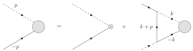
Figure 8: Feynman diagrams to renormalize the three-body composite operators $\phi\psi_{A(B)}$. The solid lines are the propagators of $\psi_{A}$ and $\psi_{B}$ fields and the dotted lines are the propagators of $\phi$ field. The shaded bulbs represent the vertex function $Z_{A(B)}(p)$.

Because of the scale invariance and in-plane rotational symmetry of the system, we can assume the form of $z_{A}({\bm{p}})$ to be

$$z_{A}({\bm{p}})=\frac{1}{\chi}\left(\frac{|{\bm{p}}|}{\Lambda}\right)^{\gamma+1},$$ (60)

where $\Lambda$ is a momentum cutoff and $\chi$ is an unknown constant. The renormalization factor becomes $Z_{\Lambda}\propto\Lambda^{-\gamma-1}$ and thus $\gamma+1$ is the anomalous dimension of the composite operator $\phi\psi_{A}$. (Here $\gamma$ and $\gamma_{l}$ appearing later are defined so that they coincide with the definition of the scaling exponents used in Ref. Nishida:2008kr .) Once $\gamma$ is determined, the scaling dimension of the renormalized composite operator $\mathcal{O}_{AAB}^{(l=0)}$ is given by

$$\Delta_{AAB}^{(l=0)}=\Delta_{\phi}+\Delta_{\psi_{A}}+\gamma+1=\frac{7}{2}+\gamma.$$ (61)

Substituting the form (60) into Eq. (59), we obtain

$$|{\bm{p}}|^{\gamma+1}=\chi\Lambda^{\gamma+1}-\frac{2\pi m_{A}}{m_{AB}\sqrt{\frac{m_{A}}{M}+1}}\int^{\Lambda}\!\!\frac{d{\bm{k}}}{(2\pi)^{2}}\frac{|{\bm{k}}|^{\gamma}}{\sqrt{\frac{m_{A}}{m_{B}}({\bm{k}}+{\bm{p}})^{2}+{\bm{k}}^{2}+{\bm{p}}^{2}}}.$$ (62)

In order for the integral to be infrared finite, $\mathrm{Re}\,(\gamma)>-2$ is necessary. Also, in order to be able to take the limit $\Lambda\to\infty$, $\mathrm{Re}\,(\gamma)<1$ is required. In the infinite cutoff limit $\Lambda\to\infty$, $\gamma$ satisfies the following equation:

$$1=-\frac{m_{A}}{m_{AB}\sqrt{\frac{m_{A}}{M}+1}}\int_{0}^{\infty}\!dk\int_{0}^{\pi}\!\frac{d\theta}{\pi}\frac{k^{\gamma+1}}{\sqrt{\left(\frac{m_{A}}{m_{B}}+1\right)k^{2}+\frac{2m_{A}}{m_{B}}k\cos\theta+\left(\frac{m_{A}}{m_{B}}+1\right)}},$$ (63)

where $k=|{\bm{k}}|/|{\bm{p}}|$ and $\cos\theta=\hat{{\bm{k}}}\cdot\hat{{\bm{p}}}$. Here the integral is understood to be evaluated where it is convergent $-2<\mathrm{Re}\,(\gamma)<-1$ and then analytically continued to an arbitrary value of $\gamma$.

Similarly, for general orbital angular momentum $l$, we consider the following three-body composite operator:

$$\mathcal{O}_{AAB}^{(l)}({\bm{x}})=Z_{\Lambda}^{-1}\sum_{j=0}^{l}c_{j}\bigl{(}\partial_{x}+i\partial_{y}\bigr{)}^{j}\phi({\bm{x}})\bigl{(}\partial_{x}+i\partial_{y}\bigr{)}^{l-j}\psi_{A}({\bm{x}}).$$ (64)

In order for $\mathcal{O}_{AAB}^{(l)}$ to be a primary operator ($[K_{i},\,\mathcal{O}_{AAB}^{(l)}]=0$), the coefficients $c_{j}$ have to be chosen so that

$$\sum_{j=0}^{l}c_{i}\left(p+\frac{M}{M+m_{A}}q\right)^{j}\left(-p+\frac{m_{A}}{M+m_{A}}q\right)^{l-j}\propto p^{l}$$ (65)

being independent of the momentum $q$ conjugate to the center-of-mass motion. In the important case of $l=1$, we easily find $c_{1}=-\frac{m_{A}}{M}c_{0}$. If we denote the anomalous dimension of such a composite operator as $\gamma_{l}+1-l$, it is straightforward to show that $\gamma_{l}$ satisfies

$$1=-\frac{m_{A}}{m_{AB}\sqrt{\frac{m_{A}}{M}+1}}\int_{0}^{\infty}\!dk\int_{0}^{\pi}\!\frac{d\theta}{\pi}\frac{\cos(l\theta)\,k^{\gamma_{l}+1}}{\sqrt{\left(\frac{m_{A}}{m_{B}}+1\right)k^{2}+\frac{2m_{A}}{m_{B}}k\cos\theta+\left(\frac{m_{A}}{m_{B}}+1\right)}}.$$ (66)

The integration over $k$ leads to the result shown in Ref. Nishida:2008kr . The scaling dimension of the renormalized composite operator $\mathcal{O}_{AAB}^{(l)}$ is given by

$$\Delta_{AAB}^{(l)}=\Delta_{\phi}+\Delta_{\psi_{A}}+l+\left(\gamma_{l}+1-l\right)=\frac{7}{2}+\gamma_{l}.$$ (67)

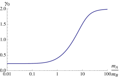
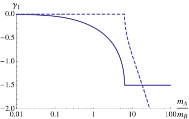
Figure 9: Anomalous dimensions $\gamma_{l}$ for $\mathcal{O}_{AAB}^{(l)}$ in the $s$-wave channel $l=0$ (left) and the $p$-wave channel $l=1$ (right) as functions of the mass ratio $m_{A}/m_{B}$ Nishida:2008kr . In the right panel, the real part of $\gamma_{1}$ (solid curve) and its imaginary part with a negative sign (dashed curve) are plotted.

The anomalous dimensions $\gamma_{l}$ obtained by solving Eq. (66) in the $s$-wave channel $l=0$ and the $p$-wave channel $l=1$ are plotted in Fig. 9 as functions of the mass ratio $m_{A}/m_{B}$. For $l=0$, $\gamma_{0}$ increases as $m_{A}/m_{B}$ is increased indicating the stronger effective repulsion in the $s$-wave channel. On the other hand, for $l=1$, $\gamma_{1}$ decreases with increasing $m_{A}/m_{B}$ and eventually becomes complex as $\gamma_{1}=-\frac{3}{2}\pm i\,\mathrm{Im}\,(\gamma_{1})$ when $m_{A}/m_{B}>6.35111$ Nishida:2008kr . (For comparison, the Born-Oppenheimer approximation predicts the critical mass ratio to be $m_{A}/m_{B}\approx 6.21791$.) In this case, using the scaling dimension $\Delta_{AAB}^{(l=1)}=2\pm i\,\mathrm{Im}\,(\gamma_{1})$ and Eq. (53), the two-point correlation function of $\mathcal{O}_{AAB}^{(l=1)}$ is found to behave as

$$\begin{split}\int\!dtd{\bm{x}}\,e^{-i{\bm{p}}\cdot{\bm{x}}+ip_{0}t}\langle T\,\mathcal{O}(t,{\bm{x}})\mathcal{O}^{\dagger}(0,{\bm{0}})\rangle&=\sum_{\pm}b_{\pm}\left[\frac{{\bm{p}}^{2}}{4m_{A}+2m_{B}}-p_{0}-i0^{+}\right]^{\pm i\,\mathrm{Im}(\gamma_{1})}\\ &\propto\sin\!\left[\mathrm{Im}(\gamma_{1})\ln\left(\frac{{\bm{p}}^{2}-(4m_{A}+2m_{B})p_{0}-i0^{+}}{\Lambda^{2}}\right)+\varphi\right].\end{split}$$ (68)

Now the full scale invariance is broken to a discrete scaling symmetry,

$${\bm{p}}\to e^{\pi/\mathrm{Im}(\gamma_{1})}\,{\bm{p}}\qquad\quad\text{and}\qquad\quad p_{0}\to e^{2\pi/\mathrm{Im}(\gamma_{1})}\,p_{0},$$ (69)

which is a characteristic of a renormalization-group limit cycle Bedaque:1998kg . This implies the existence of an infinite set of discrete bound states in the $p$-wave $AAB$ three-body system. The energy eigenvalues form a geometric spectrum as $E_{n+1}/E_{n}=e^{-2\pi/|\mathrm{Im}(\gamma_{1})|}$ and they are known as Efimov bound states in the usual 3D case Efimov:1972 . Because the system develops deep three-body bound states, the corresponding many-body system cannot be stable toward collapse.

We note that an interesting thing becomes possible in the range of mass ratio $2.32780<m_{A}/m_{B}<6.35111$ Nishida:2008kr . Here the anomalous dimension is $-\frac{3}{2}<\gamma_{1}<-\frac{1}{2}$ (see the right panel in Fig. 9) and thus the scaling dimension of the three-body composite operator $\mathcal{O}_{AAB}^{(l=1)}$ becomes $2<\Delta_{AAB}^{(l=1)}<3$. Therefore a new three-body interaction term

$$S_{\text{3-body}}=g_{1}\int\!dtd{\bm{x}}\,\mathcal{O}^{\dagger}(t,{\bm{x}})\mathcal{O}(t,{\bm{x}})$$ (70)

becomes renormalizable because now the coupling has the dimension $-2<[g_{1}]<0$ Nishida:2007mr . The action (1) with $S_{\text{3-body}}$ added defines a new renormalizable theory. In particular, when $g_{1}$ is tuned to an $AAB$ three-body resonance, the resulting system provides a novel nonrelativistic defect CFT describing two-species fermions with both two-body ($AB$) and three-body ($AAB$) resonances in the 2D-3D mixture Nishida:2008kr .

B.2.2 $ABB$ three-body operators

A three-body operator composed of one $A$ atom and two $B$ atoms with zero orbital angular momentum $l=0$ is

$$\mathcal{O}_{ABB}^{(l=0)}({\bm{x}})=Z_{\Lambda}^{-1}\phi({\bm{x}})\psi_{B}({\bm{x}},0),$$ (71)

where $Z_{\Lambda}$ is a cutoff-dependent renormalization factor. We can study the renormalization of the composite operator $\phi\psi_{B}$ by evaluating its matrix element $\langle 0|\phi\psi_{B}({\bm{x}})|p,-p\rangle$. Feynman diagrams to renormalize $\phi\psi_{B}$ is depicted in Fig. 8. The vertex function $Z_{B}(p_{0},{\bm{p}})$ in Fig. 8 satisfies the following integral equation:

$$\begin{split}Z_{B}(p_{0},{\bm{p}})&=1-i\int\!\frac{dk_{0}d{\bm{k}}}{(2\pi)^{3}}\,G_{B}(-k)G_{A}(k+p)D(k)Z_{B}(k_{0},{\bm{k}})\\ &=1-\frac{\pi}{m_{AB}}\sqrt{\frac{2}{m_{B}}}\int\!\frac{d{\bm{k}}dk_{z}}{(2\pi)^{3}}\frac{1}{\frac{({\bm{k}}+{\bm{p}})^{2}}{2m_{A}}+\frac{{\bm{k}}^{2}+k_{z}^{\,2}}{2m_{B}}-p_{0}-i0^{+}}\frac{1}{\sqrt{\frac{{\bm{k}}^{2}}{2M}+\frac{{\bm{k}}^{2}+k_{z}^{\,2}}{2m_{B}}-i0^{+}}}Z_{B}\!\left(-\frac{{\bm{k}}^{2}+k_{z}^{\,2}}{2m_{B}},{\bm{k}}\right),\end{split}$$ (72)

where we used the analyticity of $Z_{B}(k_{0},{\bm{k}})$ on the upper half plane of $k_{0}$. The minus sign in front of the second term comes from the Fermi statistics of $B$ atoms. When we set $p_{0}=-\frac{{\bm{p}}^{2}+p_{z}^{\,2}}{2m_{B}}$, $z_{B}({\bm{p}},p_{z})\equiv Z_{B}\!\left(-\frac{{\bm{p}}^{2}+p_{z}^{\,2}}{2m_{B}},{\bm{p}}\right)$ satisfies

$$\begin{split}z_{B}({\bm{p}},p_{z})&=1-\frac{4\pi m_{B}}{m_{AB}}\int\!\frac{d{\bm{k}}dk_{z}}{(2\pi)^{3}}\frac{1}{\frac{m_{B}}{m_{A}}({\bm{k}}+{\bm{p}})^{2}+{\bm{k}}^{2}+k_{z}^{\,2}+{\bm{p}}^{2}+p_{z}^{\,2}}\frac{1}{\sqrt{\frac{m_{B}}{M}{\bm{k}}^{2}+{\bm{k}}^{2}+k_{z}^{\,2}}}z_{B}({\bm{k}},k_{z}).\end{split}$$ (73)

Because of the scale invariance and in-plane rotational symmetry of the system, we can assume the form of $z_{B}({\bm{p}},p_{z})$ to be

$$z_{B}({\bm{p}},p_{z})=\left(\frac{|{\bm{p}}|}{\Lambda}\right)^{\gamma+1}S\!\left(\frac{|p_{z}|}{|{\bm{p}}|}\right),$$ (74)

where $\Lambda$ is a momentum cutoff and $S(|p_{z}|/|{\bm{p}}|)$ is an unknown function. The renormalization factor becomes $Z_{\Lambda}\propto\Lambda^{-\gamma-1}$ and thus $\gamma+1$ is the anomalous dimension of the composite operator $\phi\psi_{B}$. (Here $\gamma$ and $\gamma_{l}$ appearing later are defined so that they coincide with the definition of the scaling exponents used in Ref. Nishida:2008kr .) Once $\gamma$ is determined, the scaling dimension of the renormalized composite operator $\mathcal{O}_{ABB}^{(l=0)}$ is given by

$$\Delta_{ABB}^{(l=0)}=\Delta_{\phi}+\Delta_{\psi_{B}}+\gamma+1=4+\gamma.$$ (75)

Substituting the form (74) into Eq. (73), we obtain

$$\begin{split}|{\bm{p}}|^{\gamma+1}S\!\left(\frac{|p_{z}|}{|{\bm{p}}|}\right)&=\Lambda^{\gamma+1}-\frac{4\pi m_{B}}{m_{AB}}\int^{\Lambda}\!\frac{d{\bm{k}}dk_{z}}{(2\pi)^{3}}\frac{1}{\frac{m_{B}}{m_{A}}({\bm{k}}+{\bm{p}})^{2}+{\bm{k}}^{2}+k_{z}^{\,2}+{\bm{p}}^{2}+p_{z}^{\,2}}\frac{|{\bm{k}}|^{\gamma+1}}{\sqrt{\frac{m_{B}}{M}{\bm{k}}^{2}+{\bm{k}}^{2}+k_{z}^{\,2}}}\,S\!\left(\frac{|k_{z}|}{|{\bm{k}}|}\right).\end{split}$$ (76)

In order for the integral to be infrared finite, $\mathrm{Re}\,(\gamma)>-3$ is necessary. Also, in order to be able to take the limit $\Lambda\to\infty$, $\mathrm{Re}\,(\gamma)<1$ is required. In the infinite cutoff limit $\Lambda\to\infty$, $\gamma$ satisfies the following integral equation:

$$\begin{split}|{\bm{p}}|^{\gamma+1}S\!\left(\frac{|p_{z}|}{|{\bm{p}}|}\right)&=-\frac{4\pi m_{B}}{m_{AB}}\int_{-\infty}^{\infty}\!\frac{d{\bm{k}}dk_{z}}{(2\pi)^{3}}\frac{1}{\frac{m_{B}}{m_{A}}({\bm{k}}+{\bm{p}})^{2}+{\bm{k}}^{2}+k_{z}^{\,2}+{\bm{p}}^{2}+p_{z}^{\,2}}\frac{|{\bm{k}}|^{\gamma+1}}{\sqrt{\frac{m_{B}}{M}{\bm{k}}^{2}+{\bm{k}}^{2}+k_{z}^{\,2}}}\,S\!\left(\frac{|k_{z}|}{|{\bm{k}}|}\right).\end{split}$$ (77)

Here the integral is understood to be evaluated where it is convergent $-3<\mathrm{Re}\,(\gamma)<-1$ and then analytically continued to an arbitrary value of $\gamma$.

Similarly, for general orbital angular momentum $l$, we consider the following three-body composite operator:

$$\mathcal{O}_{ABB}^{(l)}({\bm{x}})=Z_{\Lambda}^{-1}\sum_{j=0}^{l}c_{j}\bigl{(}\partial_{x}+i\partial_{y}\bigr{)}^{j}\phi({\bm{x}})\bigl{(}\partial_{x}+i\partial_{y}\bigr{)}^{l-j}\psi_{B}({\bm{x}}).$$ (78)

In order for $\mathcal{O}_{ABB}^{(l)}$ to be a primary operator ($[K_{i},\,\mathcal{O}_{ABB}^{(l)}]=0$), the coefficients $c_{j}$ have to be chosen so that

$$\sum_{j=0}^{l}c_{i}\left(p+\frac{M}{M+m_{B}}q\right)^{j}\left(-p+\frac{m_{B}}{M+m_{B}}q\right)^{l-j}\propto p^{l}$$ (79)

being independent of the momentum $q$ conjugate to the center-of-mass motion. In the important case of $l=1$, we easily find $c_{1}=-\frac{m_{B}}{M}c_{0}$. If we denote the anomalous dimension of such a composite operator as $\gamma_{l}+1-l$, it is straightforward to show that $\gamma_{l}$ satisfies

$$\begin{split}|{\bm{p}}|^{\gamma_{l}+1}S_{l}\!\left(\frac{|p_{z}|}{|{\bm{p}}|}\right)&=-\frac{4\pi m_{B}}{m_{AB}}\int_{-\infty}^{\infty}\!\frac{d{\bm{k}}dk_{z}}{(2\pi)^{3}}\frac{\cos\bigl{(}l\theta_{\hat{{\bm{k}}}\cdot\hat{{\bm{p}}}}\bigr{)}}{\frac{m_{B}}{m_{A}}({\bm{k}}+{\bm{p}})^{2}+{\bm{k}}^{2}+k_{z}^{\,2}+{\bm{p}}^{2}+p_{z}^{\,2}}\frac{|{\bm{k}}|^{\gamma_{l}+1}}{\sqrt{\frac{m_{B}}{M}{\bm{k}}^{2}+{\bm{k}}^{2}+k_{z}^{\,2}}}\,S_{l}\!\left(\frac{|k_{z}|}{|{\bm{k}}|}\right).\end{split}$$ (80)

Rescalings of the variables ${\bm{k}}\to\sqrt{\frac{m_{A}}{M}}{\bm{k}}$ and ${\bm{p}}\to\sqrt{\frac{m_{A}}{M}}{\bm{p}}$ and redefinition of the unknown function $S_{l}(|p_{z}|/|{\bm{p}}|)$ lead to the result shown in Ref. Nishida:2008kr . The scaling dimension of the renormalized composite operator $\mathcal{O}_{ABB}^{(l)}$ is given by

$$\Delta_{ABB}^{(l)}=\Delta_{\phi}+\Delta_{\phi_{B}}+l+\left(\gamma_{l}+1-l\right)=4+\gamma_{l}.$$ (81)

By solving the integral equation (80) numerically, we find that the anomalous dimension $\gamma_{1}$ in the $p$-wave channel $l=1$ decreases with decreasing the mass ratio $m_{A}/m_{B}$ and eventually becomes complex as $\gamma_{1}=-2\pm i\,\mathrm{Im}\,(\gamma_{1})$ when $m_{A}/m_{B}<0.0351287$ Nishida:2008kr . This implies the existence of the Efimov bound states in the $p$-wave $ABB$ three-body system [see discussions about Eqs. (68) and (69)]. Furthermore, in the range of mass ratio $0.0351287<u<0.0660841$ Nishida:2008kr , the anomalous dimension is $-2<\gamma_{1}<-1$ and thus the scaling dimension of the three-body composite operator $\mathcal{O}_{ABB}^{(l=1)}$ becomes $2<\Delta_{ABB}^{(l=1)}<3$. As a consequence, an additional $ABB$ three-body resonance can be introduced and the resulting system provides a novel nonrelativistic defect CFT describing two-species fermions with both two-body ($AB$) and three-body ($ABB$) resonances in the 2D-3D mixture [see discussions about Eq. (70)].

It would be difficult to determine scaling dimensions of composite operators with particles more than three. However, it is possible to estimate them by numerically solving the energy eigenvalue problems of $H_{\mathrm{osc}}$ with the help of the operator-state correspondence (50) or by using the analytic $\epsilon$ expansions around the special dimensions $d_{B}\to 4$ and $d_{B}\to 2$ (see Sec. III.5) Nishida:2007pj .

B.3 Operator product expansions

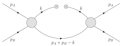
Figure 10: Feynman diagram evaluated in Eqs. (83) and (90). The solid lines are the propagators of $\psi_{A}$ and $\psi_{B}$ fields and the shaded bulbs represent the two-particle scattering amplitude $i\mathcal{A}(p_{A}+p_{B})$.

Here we consider an arbitrary effective scattering length $-\infty<a_{\mathrm{eff}}^{-1}<\infty$ and study operator product expansions (OPEs) in our defect quantum field theory (1). We first work on the following OPE:

$$\psi_{A}^{\dagger}\!\left({\bm{x}}-\frac{{\bm{y}}}{2}\right)\psi_{A}\!\left({\bm{x}}+\frac{{\bm{y}}}{2}\right)=\sum_{n}W_{A,n}({\bm{y}})\mathcal{O}_{n}({\bm{x}}).$$ (82)

Here $W_{A,n}({\bm{y}})$ are Wilson coefficients and $\mathcal{O}_{n}({\bm{x}})$ are renormalized defect operators. We remind that ${\bm{x}}$ and ${\bm{y}}$ are two-dimensional coordinates on the defect. We can determine the lowest three $W_{A,n}$ and $\mathcal{O}_{n}$ by evaluating the matrix elements of the both sides of Eq. (82) between two-particle states $\langle p_{A},p_{B}|$ and $|p_{A},p_{B}\rangle$. According to Ref. Braaten:2008uh , we shall consider the Feynman diagram depicted in Fig. 10 that has nonanalyticity at $|{\bm{y}}|=0$. By denoting the total energy and momentum as $p=p_{A}+p_{B}$, the matrix element of the left-hand side of Eq. (82) becomes

$$\begin{split}\left\langle\psi_{A}^{\dagger}\!\left({\bm{x}}-\frac{{\bm{y}}}{2}\right)\psi_{A}\!\left({\bm{x}}+\frac{{\bm{y}}}{2}\right)\right\rangle_{\mathrm{fig:\ref{fig:ope}}}&=[i\mathcal{A}(p)]^{2}\int\!\frac{dk_{0}d{\bm{k}}}{(2\pi)^{3}}\,e^{i{\bm{k}}\cdot{\bm{y}}}\,iG_{A}(k)iG_{A}(k)iG_{B}(p-k)\\ &=\frac{m_{B}m_{AB}}{2\pi\sqrt{-2m_{B}\mathcal{E}_{p}}}\mathcal{A}(p)^{2}e^{i\frac{m_{A}}{M}{\bm{p}}\cdot{\bm{y}}-|{\bm{y}}|\sqrt{-2m_{AB}\mathcal{E}_{p}}}.\end{split}$$ (83)

Here $\mathcal{A}(p)$ is the two-particle scattering amplitude given in Eq. (7) and we introduced a shorthand notation $\mathcal{E}_{p}\equiv p_{0}-\frac{{\bm{p}}^{2}}{2M}+i0^{+}$. If we expand the exponential in terms of $|{\bm{y}}|$, the terms with odd powers of $|{\bm{y}}|$ are nonanalytic at $|{\bm{y}}|=0$:

$$\begin{split}\left\langle\psi_{A}^{\dagger}\!\left({\bm{x}}-\frac{{\bm{y}}}{2}\right)\psi_{A}\!\left({\bm{x}}+\frac{{\bm{y}}}{2}\right)\right\rangle_{\mathrm{fig:\ref{fig:ope}}}&=\frac{m_{B}m_{AB}}{2\pi\sqrt{-2m_{B}\mathcal{E}_{p}}}\mathcal{A}(p)^{2}e^{i\frac{m_{A}}{M}{\bm{p}}\cdot{\bm{y}}}-\frac{m_{AB}\sqrt{m_{B}m_{AB}}}{2\pi}\mathcal{A}(p)^{2}|{\bm{y}}|+O({\bm{y}}^{2}).\end{split}$$ (84)

The first term expanded in powers of ${\bm{y}}$ can be easily identified with the Taylor series of the left-hand side:

$$\frac{m_{B}m_{AB}}{2\pi\sqrt{-2m_{B}\mathcal{E}_{p}}}\mathcal{A}(p)^{2}e^{i\frac{m_{A}}{M}{\bm{p}}\cdot{\bm{y}}}=\langle\psi_{A}^{\dagger}\psi_{A}({\bm{x}})\rangle_{\mathrm{fig:\ref{fig:ope}}}+\frac{{\bm{y}}}{2}\cdot\langle\psi_{A}^{\dagger}\tensor{\bm{\nabla}}\psi_{A}({\bm{x}})\rangle_{\mathrm{fig:\ref{fig:ope}}}+\cdots.$$ (85)

Below we will show that the second term in Eq. (84) can be identified with the matrix element of the defect operator; $\psi_{A}^{\dagger}\psi_{B}^{\dagger}\psi_{B}\psi_{A}({\bm{x}})\equiv\psi_{A}^{\dagger}({\bm{x}})\psi_{B}^{\dagger}({\bm{x}},0)\psi_{B}({\bm{x}},0)\psi_{A}({\bm{x}})$.

The matrix element of $\psi_{A}^{\dagger}\psi_{B}^{\dagger}\psi_{B}\psi_{A}({\bm{x}})$ between the same two-particle states $\langle p_{A},p_{B}|$ and $|p_{A},p_{B}\rangle$ is evaluated as

$$\langle\psi_{A}^{\dagger}\psi_{B}^{\dagger}\psi_{B}\psi_{A}({\bm{x}})\rangle=\left[1+i\mathcal{A}(p)\int\!\frac{dk_{0}d{\bm{k}}}{(2\pi)^{3}}\,iG_{A}(p-k)iG_{B}(k)\right]^{2}\\ =\frac{\mathcal{A}(p)^{2}}{g_{0}^{\,2}},$$ (86)

where we used Eq. (4). By comparing Eq. (86) with the second term in Eq. (84), we find the OPE of $\psi_{A}^{\dagger}\!\left({\bm{x}}-\frac{{\bm{y}}}{2}\right)\psi_{A}\!\left({\bm{x}}+\frac{{\bm{y}}}{2}\right)$ to be

$$\psi_{A}^{\dagger}\!\left({\bm{x}}-\frac{{\bm{y}}}{2}\right)\psi_{A}\!\left({\bm{x}}+\frac{{\bm{y}}}{2}\right)=\psi_{A}^{\dagger}\psi_{A}({\bm{x}})+\frac{{\bm{y}}}{2}\cdot\psi_{A}^{\dagger}\tensor{\bm{\nabla}}\psi_{A}({\bm{x}})-\frac{m_{AB}\sqrt{m_{B}m_{AB}}}{2\pi}|{\bm{y}}|\,g_{0}^{\,2}\psi_{A}^{\dagger}\psi_{B}^{\dagger}\psi_{B}\psi_{A}({\bm{x}})+O({\bm{y}}^{2}).$$ (87)

Here $g_{0}^{\,2}\psi_{A}^{\dagger}\psi_{B}^{\dagger}\psi_{B}\psi_{A}({\bm{x}})$ is the renormalized defect operator having finite matrix elements. This result is a generalization of the OPE studied in the usual 3D case in Ref. Braaten:2008uh to our 2D-3D mixture. In particular, the existence of the nonanalytic term in $|{\bm{y}}|$ implies that the two-dimensional momentum distribution of $A$ atoms has the following large-momentum tail:

$$\begin{split}\rho_{A}(|{\bm{k}}|)&=\int\!d{\bm{y}}\,e^{-i{\bm{k}}\cdot{\bm{y}}}\left\langle\psi_{A}^{\dagger}\!\left({\bm{x}}-\frac{{\bm{y}}}{2}\right)\psi_{A}\!\left({\bm{x}}+\frac{{\bm{y}}}{2}\right)\right\rangle_{\text{any}}\\ &\to\frac{m_{AB}\sqrt{m_{B}m_{AB}}}{|{\bm{k}}|^{3}}\langle g_{0}^{\,2}\psi_{A}^{\dagger}\psi_{B}^{\dagger}\psi_{B}\psi_{A}({\bm{x}})\rangle_{\text{any}}\qquad(|{\bm{k}}|\to\infty).\end{split}$$ (88)

Here the expectation value can be taken with any state in the system, for example, at finite densities of $A$ and $B$ atoms and at finite temperature. The quantity in the right-hand side is called the contact density and given by $\langle g_{0}^{\,2}\psi_{A}^{\dagger}\psi_{B}^{\dagger}\psi_{B}\psi_{A}({\bm{x}})\rangle_{\mathrm{any}}\to 4\pi^{2}a_{\mathrm{eff}}^{\,2}\,n_{A}n_{B}/(m_{B}m_{AB})$ in the weak coupling limit $a_{\mathrm{eff}}\to-0$. The coefficient of the large-momentum tail has played an important role in the exact analysis of the unitary Fermi gas in pure 3D Tan:2005 . It is an important future problem to investigate exact relationships in our 2D-3D mixed dimensions.

The following OPE will be more interesting because it involves the $z$-direction perpendicular to the 2D defect:

$$\psi_{B}^{\dagger}\!\left({\bm{x}}-\frac{{\bm{y}}}{2},z\right)\psi_{B}\!\left({\bm{x}}+\frac{{\bm{y}}}{2},z\right)=\sum_{n}W_{B,n}({\bm{y}},z)\mathcal{O}_{n}({\bm{x}}).$$ (89)

Wilson coefficients $W_{B,n}({\bm{y}},z)$ and renormalized defect operators $\mathcal{O}_{n}({\bm{x}})$ can be determined by evaluating the matrix elements of the both sides of Eq. (89) between the two-particle states $\langle p_{A},p_{B}|$ and $|p_{A},p_{B}\rangle$. We shall consider the Feynman diagram depicted in Fig. 10 again that has nonanalyticity at $|{\bm{y}}|=|z|=0$. The matrix element of the left-hand side of Eq. (89) becomes

$$\begin{split}\left\langle\psi_{B}^{\dagger}\!\left({\bm{x}}-\frac{{\bm{y}}}{2},z\right)\psi_{B}\!\left({\bm{x}}+\frac{{\bm{y}}}{2},z\right)\right\rangle_{\mathrm{fig:\ref{fig:ope}}}&=[i\mathcal{A}(p)]^{2}\int\!\frac{dk_{0}d{\bm{k}}}{(2\pi)^{3}}\,e^{i{\bm{k}}\cdot{\bm{y}}}\,iG_{B}(k;z)iG_{B}(k;-z)iG_{A}(p-k)\\ &=m_{B}m_{AB}\mathcal{A}(p)^{2}e^{i\frac{m_{B}}{M}{\bm{p}}\cdot{\bm{y}}}\int\!\frac{d{\bm{k}}}{(2\pi)^{2}}\frac{e^{i{\bm{k}}\cdot{\bm{y}}-2|z|\sqrt{\frac{m_{B}}{m_{AB}}{\bm{k}}^{2}-2m_{B}\mathcal{E}_{p}}}}{{\bm{k}}^{2}-2m_{AB}\mathcal{E}_{p}}.\end{split}$$ (90)

When $|z|\neq 0$ is fixed, the right-hand side is analytic in terms of ${\bm{y}}$ and therefore the OPE of $\psi_{B}^{\dagger}\!\left({\bm{x}}-\frac{{\bm{y}}}{2},z\right)\psi_{B}\!\left({\bm{x}}+\frac{{\bm{y}}}{2},z\right)$ is simply given by its Taylor series in powers of ${\bm{y}}$. This is natural because there is no interaction with $\psi_{A}({\bm{x}})$ away from the 2D defect located at $z=0$.

We now set ${\bm{y}}={\bm{0}}$ and study the OPE of $\psi_{B}^{\dagger}\psi_{B}({\bm{x}},z)\equiv\psi_{B}^{\dagger}({\bm{x}},z)\psi_{B}({\bm{x}},z)$ as a function of the distance from the 2D defect $|z|$ (termed defect operator product expansion). Performing the integration over ${\bm{k}}$ in Eq. (90) with ${\bm{y}}={\bm{0}}$, we obtain

$$\begin{split}\langle\psi_{B}^{\dagger}\psi_{B}({\bm{x}},z)\rangle_{\mathrm{fig:\ref{fig:ope}}}&=-\frac{m_{B}m_{AB}}{2\pi}\mathcal{A}(p)^{2}\,\mathrm{Ei}\!\left(-2|z|\sqrt{-2m_{B}\mathcal{E}_{p}}\right)\\ &=-\frac{m_{B}m_{AB}}{2\pi}\mathcal{A}(p)^{2}\ln\!\left(2\,e^{\gamma_{\mathrm{E}}}|z|\sqrt{-2m_{B}\mathcal{E}_{p}}\right)+O(|z|),\end{split}$$ (91)

where $\mathrm{Ei}(x)\equiv\int_{-x}^{\infty}\!\frac{dt}{t}e^{-t}$. We can identify the lowest order term in the right-hand side with

$$-\frac{m_{B}m_{AB}}{2\pi}\mathcal{A}(p)^{2}\ln\!\left(2\,e^{\gamma_{\mathrm{E}}}|z|\sqrt{-2m_{B}\mathcal{E}_{p}}\right)=\langle\psi_{B}^{\dagger}\psi_{B}({\bm{x}},0)\rangle^{(\lambda)}_{\mathrm{fig:\ref{fig:ope}}}-\frac{m_{B}m_{AB}}{2\pi}\ln\left(2\,e^{\gamma_{\mathrm{E}}}|z|\lambda\right)\langle g_{0}^{\,2}\psi_{A}^{\dagger}\psi_{B}^{\dagger}\psi_{B}\psi_{A}({\bm{x}})\rangle,$$ (92)

where $\lambda$ is an arbitrary momentum scale. Therefore we find the defect OPE of $\psi_{B}^{\dagger}\psi_{B}({\bm{x}},z)$ to be

$$\psi_{B}^{\dagger}\psi_{B}({\bm{x}},z)=\psi_{B}^{\dagger}\psi_{B}({\bm{x}},0)^{(\lambda)}-\frac{m_{B}m_{AB}}{2\pi}\ln\left(2\,e^{\gamma_{\mathrm{E}}}|z|\lambda\right)\,g_{0}^{\,2}\psi_{A}^{\dagger}\psi_{B}^{\dagger}\psi_{B}\psi_{A}({\bm{x}})+O(|z|).$$ (93)

Because $\psi_{B}^{\dagger}\psi_{B}({\bm{x}},z)$ is the density operator of $B$ atoms, the above result suggests that the density of $B$ atoms diverges logarithmically toward the 2D defect $|z|\to 0$:

$$\tilde{n}_{B}(|z|)=\langle\psi_{B}^{\dagger}\psi_{B}({\bm{x}},z)\rangle_{\mathrm{any}}\to-\frac{m_{B}m_{AB}}{2\pi}\ln|z|\,\langle g_{0}^{\,2}\psi_{A}^{\dagger}\psi_{B}^{\dagger}\psi_{B}\psi_{A}({\bm{x}})\rangle_{\mathrm{any}}.$$ (94)

The coefficient of the divergence is given by the contact density up to the mass-dependent factor. Further analysis to elucidate this aspect will be worthwhile.

B.4 Conclusion

Two-species fermions in the 2D-3D mixed dimensions in the unitarity limit can be regarded as a nonrelativistic defect CFT. We derived the reduced Schrödinger algebra and the operator-state correspondence in general nonrelativistic defect CFTs. We also studied scaling dimensions of few-body composite operators and operator product expansions in our 2D-3D mixture. In particular, for the stability of the many-body system near the unitarity limit, we showed that the mass ratio has to be in the range $0.0351287<m_{\mathrm{2D}}/m_{\mathrm{3D}}<6.35111$ to avoid the Efimov effect Nishida:2008kr . Finally, we emphasize that all field-theoretical methods presented here to determine scaling dimensions and critical mass ratios are widely applicable to both fermionic and bosonic systems and also in the 1D-3D mixture Nishida:2008kr and in the usual 3D case Nishida:2007pj ; Nishida:2007mr ; Mehen:2007dn .

References

- (1) W. Ketterle and M. W. Zwierlein, Proceedings of the International School of Physics “Enrico Fermi”, Varenna, (IOS Press, 2008); arXiv:0801.2500 [cond-mat.other], and references therein.
- (2) For recent theoretical reviews, see I. Bloch, J. Dalibard, and W. Zwerger, Rev. Mod. Phys. 80, 885 (2008); S. Giorgini, L. P. Pitaevskii, and S. Stringari, Rev. Mod. Phys. 80, 1215 (2008).
- (3) N. Read and D. Green, Phys. Rev. B 61, 10267 (2000).
- (4) S. Tewari, S. Das Sarma, C. Nayak, C. Zhang, and P. Zoller, Phys. Rev. Lett. 98, 010506 (2007).
- (5) J. L. Bohn, Phys. Rev. A 61, 053409 (2000).
- (6) T.-L. Ho and R. B. Diener, Phys. Rev. Lett. 94, 090402 (2005).
- (7) Y. Ohashi, Phys. Rev. Lett. 94, 050403 (2005).
- (8) V. Gurarie, L. Radzihovsky, and A. V. Andreev, Phys. Rev. Lett. 94, 230403 (2005).
- (9) S. S. Botelho and C. A. R. Sá de Melo, J. Low Temp. Phys. 140, 409 (2005).
- (10) C.-H. Cheng and S.-K. Yip, Phys. Rev. Lett. 95, 070404 (2005); Phys. Rev. B 73, 064517 (2006).
- (11) M. Iskin and C. A. R. Sá de Melo, Phys. Rev. Lett. 96, 040402 (2006).
- (12) L. You and M. Marinescu, Phys. Rev. A 60, 2324 (1999).
- (13) D. V. Efremov, M. S. Mar’enko, M. A. Baranov, and M. Y. Kagan, Sov. Phys. JETP 90, 861 (2000).
- (14) D. V. Efremov and L. Viverit, Phys. Rev. B 65, 134519 (2002).
- (15) S. Gaudio, J. Jackiewicz, and K. S. Bedell, Phil. Mag. Lett. 87, 713 (2007).
- (16) A. Bulgac, M. M. Forbes, and A. Schwenk, Phys. Rev. Lett. 97, 020402 (2006).
- (17) C. Zhang, S. Tewari, R. M. Lutchyn, and S. Das Sarma, Phys. Rev. Lett. 101, 160401 (2008).
- (18) C. A. Regal, C. Ticknor, J. L. Bohn, and D. S. Jin, Phys. Rev. Lett. 90, 053201 (2003).
- (19) J. Zhang, E. G. M. van Kempen, T. Bourdel, L. Khaykovich, J. Cubizolles, F. Chevy, M. Teichmann, L. Tarruell, S. J. J. M. F. Kokkelmans, and C. Salomon, Phys. Rev. A 70, 030702 (2004).
- (20) C. H. Schunck, M. W. Zwierlein, C. A. Stan, S. M. F. Raupach, and W. Ketterle, Phys. Rev. A 71, 045601 (2005).
- (21) K. Günter, T. Stöferle, H. Moritz, M. Köhl, and T. Esslinger, Phys. Rev. Lett. 95, 230401 (2005).
- (22) J. P. Gaebler, J. T. Stewart, J. L. Bohn, and D. S. Jin, Phys. Rev. Lett. 98, 200403 (2007).
- (23) D. S. Jin, J. P. Gaebler, and J. T. Stewart, Proceedings of the International Conference on Laser Spectroscopy, Telluride, Colorado, (World Scientific, 2008).
- (24) J. Fuchs, C. Ticknor, P. Dyke, G. Veeravalli, E. Kuhnle, W. Rowlands, P. Hannaford, and C. J. Vale, Phys. Rev. A 77, 053616 (2008).
- (25) Y. Inada, M. Horikoshi, S. Nakajima, M. Kuwata-Gonokami, M. Ueda, and T. Mukaiyama, Phys. Rev. Lett. 101, 100401 (2008).
- (26) D. S. Petrov, C. Salomon, and G. V. Shlyapnikov, Phys. Rev. Lett. 93, 090404 (2004); Phys. Rev. A 71, 012708 (2005); J. Phys. B 38, S645 (2005).
- (27) J. Levinsen, N. R. Cooper, and V. Gurarie, Phys. Rev. Lett. 99, 210402 (2007); arXiv:0808.1304 [cond-mat.supr-con].
- (28) M. Jona-Lasinio, L. Pricoupenko, and Y. Castin, Phys. Rev. A 77, 043611 (2008).
- (29) Y. Nishida and S. Tan, Phys. Rev. Lett. 101, 170401 (2008).
- (30) M. Taglieber, A.-C. Voigt, T. Aoki, T. W. Hänsch, and K. Dieckmann, Phys. Rev. Lett. 100, 010401 (2008).
- (31) E. Wille, F. M. Spiegelhalder, G. Kerner, D. Naik, A. Trenkwalder, G. Hendl, F. Schreck, R. Grimm, T. G. Tiecke, J. T. M. Walraven, S. J. J. M. F. Kokkelmans, E. Tiesinga, and P. S. Julienne, Phys. Rev. Lett. 100, 053201 (2008).
- (32) V. Peano, M. Thorwart, C. Mora, and R. Egger, New J. Phys. 7, 192 (2005).
- (33) P. Massignan and Y. Castin, Phys. Rev. A 74, 013616 (2006).
- (34) P. W. Anderson and P. Morel, Phys. Rev. 123, 1911 (1961).
- (35) C. Ticknor, C. A. Regal, D. S. Jin, and J. L. Bohn, Phys. Rev. A 69, 042712 (2004).
- (36) Y. Nishida and D. T. Son, Phys. Rev. Lett. 97, 050403 (2006).
- (37) Y. Nishida and D. T. Son, Phys. Rev. A 75, 063617 (2007).
- (38) Y. Nishida, Phys. Rev. A 75, 063618 (2007).
- (39) Y. Nishida, Ph. D. Thesis, University of Tokyo, 2007 [available as arXiv:cond-mat/0703465].
- (40) P. Nikolic and S. Sachdev, Phys. Rev. A 75, 033608 (2007).
- (41) M. Y. Veillette, D. E. Sheehy, and L. Radzihovsky, Phys. Rev. A 75, 043614 (2007).
- (42) L. He and P. Zhuang, Phys. Rev. A 78, 033613 (2008).
- (43) See, e. g., R. Maartens, Living Rev. Rel. 7, 7 (2004).
- (44) T. Mehen, I. W. Stewart, and M. B. Wise, Phys. Lett. B 474, 145 (2000).
- (45) R. Jackiw and S.-Y. Pi, Phys. Rev. D 42, 3500 (1990) [Erratum-ibid. D 48, 3929 (1993)].
- (46) Y. Nishida, Phys. Rev. D 77, 061703 (2008).
- (47) Y. Nishida, D. T. Son, and S. Tan, Phys. Rev. Lett. 100, 090405 (2008).
- (48) D. T. Son, Phys. Rev. D 78, 046003 (2008).
- (49) K. Balasubramanian and J. McGreevy, Phys. Rev. Lett. 101, 061601 (2008).
- (50) J. L. Cardy, Nucl. Phys. B 240, 514 (1984).
- (51) D. M. McAvity and H. Osborn, Nucl. Phys. B 455, 522 (1995).
- (52) Y. Nishida and D. T. Son, Phys. Rev. D 76, 086004 (2007).
- (53) F. Werner and Y. Castin, Phys. Rev. A 74, 053604 (2006).
- (54) M. Henkel, J. Statist. Phys. 75, 1023 (1994).
- (55) P. F. Bedaque, H.-W. Hammer, and U. van Kolck, Phys. Rev. Lett. 82, 463 (1999); Nucl. Phys. A 646, 444 (1999).
- (56) V. Efimov, Sov. Phys. JETP Lett. 16, 34 (1972); Nucl. Phys. A 210, 157 (1973).
- (57) E. Braaten and L. Platter, Phys. Rev. Lett. 100, 205301 (2008). E. Braaten, D. Kang, and L. Platter, Phys. Rev. A 78, 053606 (2008).
- (58) S. Tan, Ann. Phys. 323, 2952 (2008); Ann. Phys. 323, 2971 (2008); Ann. Phys. 323, 2987 (2008).
- (59) T. Mehen, Phys. Rev. A 78, 013614 (2008).