How Delicate is Brane-Antibrane Inflation?

Abstract

We systematically explore the parameter space of the state-of-the-art brane-antibrane inflation model (Baumann et al., arXiv:0706.0360, arXiv:0705.3837) which is one of the most rigorously derived from string theory, applying the cosmic background explorer normalization and constraint on the spectral index. We improve on previous treatments of uplifting by antibranes and show that the contributions from noninflationary throats play an important role in achieving a flat inflationary potential. To quantify the degree of fine-tuning needed by the model, we define an effective volume in the part of parameter space which is consistent with experimental constraints, and using Monte Carlo methods to search for a set of optimal parameters, we show that the degree of fine-tuning is alleviated by 8 orders of magnitude relative to a fiducial point which has previously been considered. In fact, close to the optimal parameter values, fine-tuning is no longer needed for any of the parameters. We show that in this natural region of the parameter space, larger values of $n_{s}$ close to $0.99$ (still within 2$\sigma$ of the WMAP5 central value) are favored, giving a new aspect of testability to the model.

I Introduction

Brane-antibrane inflation is one of the most distinctive and highly developed applications of string theory to cosmology. Although the basic idea seems simple—getting inflation from the potential between a brane and antibrane which are separated along an extra dimension—making it work has proved to be quite challenging. The earliest versions were incomplete due to the lack of an explicit mechanism for stabilizing the moduli, notably those associated with the size and shape of the extra dimensions. Major progress in this respect was made in Ref. KKLMMT , where warped compactification of type IIB string theory using the Klebanov-Strassler throat KS was exploited.

In Ref. KKLMMT , it was shown that the potential for a brane falling down the throat suffers from the $\eta$ problem: the curvature of the inflaton potential is generically of order $H^{2}$, making it too steep for inflation. To counteract this, the generically large inflaton mass must be tuned to a small value using a canceling contribution from the $F$-term potential, coming from the superpotential

$$W=W_{0}+A_{0}(\phi)e^{-aT},$$ (1)

where $\phi$ denotes the brane position (inflaton) and $T$ is the complex Kähler modulus, whose real part $\sigma$ determines the overall volume of the extra dimensions. The second term arises from nonperturbative physics like gaugino condensation on a D7-brane, which is one of the essential ingredients of the compactification. The existence of the $F$-term potential was already known to be necessary for stabilizing $T$ KKLT ; however the dependence of $A_{0}$ on $\phi$ was not known by the authors of Ref. KKLMMT ; they merely parametrized this dependence.

The actual dependence $A_{0}(\phi)$ however is calculable within string theory, and this missing step was carried out in Ref. Baumann:2006th . It was subsequently shown BCDF that the explicit form of $A_{0}(\phi)$ was apparently not amenable to achieving the desired cancellation to get a small inflaton mass. However this conclusion depended on exactly how the D7-brane was embedded in the throat. A different embedding was considered in Refs. Krause ; Baumann:2007np ; Baumann which yielded the desired form of the $F$-term potential. With sufficient tuning of parameters, it was possible to achieve inflation. Because of this need for substantial tuning, the scenario was dubbed “delicate” in Refs. Baumann:2007np ; Baumann . The difficulties were further elaborated in Ref. Panda , which surprisingly concluded that it was difficult to satisfy both the cosmic background explorer (COBE) normalization and the constraint on the spectral index. Normally one expects that there is enough freedom to adjust the overall scale of the potential to achieve the normalization of the amplitude, and indeed, we will show that satisfying the normalization presents no extraordinary new difficulty.

On the other hand, we do point out an additional challenge which was not consistently treated in previous work. Namely, it is necessary for the cosmological constant to vanish at the end of inflation. In Ref. Baumann , sufficient flatness of the potential was achieved by tuning the parameter $s$, which is the ratio of the uplifting energy to the absolute value of the negative energy of the anti-de Sitter (AdS) minimum in the absence of uplifting. In fact, this ratio is fixed (to approximately unity) by the necessity to uplift to a Minkowski minimum, thereby removing it as a tunable parameter. We take advantage of the fact that its tunability can be restored by considering the contributions from other throats to the uplifting.

In Refs. Baumann:2007np ; Baumann , it is claimed that the brane-antibrane inflationary model must be rather finely tuned. However, there is little quantitative basis for this statement. Part of our objective is to invent a quantitative measure of the degree of tuning. We propose a measure of tuning via the relative volume of parameter space around a given point, which is consistent with inflation. This statistic allows us to say to what fractional precision the parameters have to be adjusted in order to get inflation consistent with observations; e.g., parameter $x$ must be tuned to one part in 100, parameter $y$ to one part in 1000, etc. Using this measure, we show that indeed, the model is quite fine-tuned at the parameter values which have been previously suggested. However, we will show that there exists a more favorable set of parameters around which the tuning problem is much less severe, by adapting Monte Carlo methods which have been widely used in other cosmological applications for this purpose. We also consider the degree of fine-tuning using an alternative measure—the absolute volume of the allowed parameter space; we compare the two measures and show that the improvements in fine-tuning are of the same order.

A further delicate aspect of the model is the problem of overshooting the flat part of the potential by starting too high Underwood:2008dh . With the wrong initial conditions, the inflaton gathers too much speed to roll slowly in the flat region of the potential. We investigate the scope of initial conditions which is compatible with inflation and show that this aspect of the tuning problem is also improved somewhat in the most favorable parameter range.

A final technical issue concerns the extent to which the model can be treated in terms of a single field, due to the fact that the trajectory curves in the space of $\phi$, the brane modulus, and $T$, the Kähler modulus. A seemingly reasonable treatment, involving both fields plus an analytic approximation for the dependence of $T$ on $\phi$, can result in an incorrect prediction for the spectral index. We show that the single-field approximation can be a good one, provided one is sufficiently careful.

II The Potential of $D$-Brane Inflation

The inflaton potential derived by Baumann et al. Baumann:2007np ; Baumann consists of two contributions: a supersymmetric (SUSY) $F$-term potential $V_{F}$, and a SUSY-breaking contribution due to anti-D3-branes, $V_{D}$, which is necessary for uplifting the minimum from a negative value (an AdS minimum) to zero. $V_{F}$ depends on the correction to the nonperturbative superpotential,

$$A_{0}(\phi)=A_{0}\,g^{1/n}(\phi)\equiv A_{0}\left[1+\left(\phi\over\phi_{\mu}\right)^{3/2}\right]^{1/n}.$$ (2)

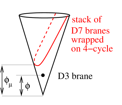
$A_{0}$ is now taken to be a constant, $n$ is the number of D7-branes in the stack, and $\phi_{\mu}$ is proportional to the radial position where the D7-brane stack comes closest to the bottom of the throat. For $\phi<\phi_{\mu}$, the D3-brane is below the D7-brane stack in the throat; this is the region where inflation takes place. The configuration is illustrated in Fig. 1.

Figure 1: Schematic representation of D7-brane stack and D3-brane in Klebanov-Strassler throat.

The dynamical degrees of freedom are expressed in terms of the dimensionless rescalings of the D3-brane modulus $\phi$ and the Kähler modulus $\sigma$,

$$x \equiv {\phi\over\phi_{\mu}},$$ (3)

$$\omega \equiv a\sigma\equiv{2\pi\over n}\sigma.$$ (4)

The potential is then

$$V(x,\omega) = V_{F}(x,\omega)+V_{D}(x,\omega),$$ (5)

$$V_{F}(x,\omega) = \frac{a|A_{0}|^{2}}{3U^{2}(x,\omega)}e^{-2\omega}g^{2/n}\left[2\omega+6-6\left|{W_{0}\over A_{0}}\right|e^{\omega}g^{-1/n}+\frac{3}{ng}\left({cx\over g}-x^{3/2}\right)\right],$$ (6)

$$V_{D}(x,\omega) = \frac{D(x)}{U^{2}(x,\omega)},$$ (7)

where $c=9/(4n\omega_{0}\phi_{\mu}^{2})$, and $\omega_{0}$ is defined to be the stable value of $\omega$ when $x=0$, i.e.,

$$\left.{\partial V\over\partial\omega}\right|_{x=0,\omega=\omega_{0}}=0.$$ (8)

Thus $\omega_{0}$ is not a free parameter. (See Appendix A.1 for details.) The functions $U$ and $D$ come from the Kähler potential and the brane-antibrane Coulombic interaction, respectively, and are given by

$$U(x,\omega) = {1\over a}\left(2\omega-{1\over 3}\omega_{0}\phi_{\mu}^{2}x^{2}\right),$$ (9)

$$D(x) = \frac{D_{0}}{1+C_{D}\displaystyle{D_{0}\over x^{4}}}+D_{1},\qquad C_{D}={27\over 64\pi^{2}\phi_{\mu}^{4}}.$$ (10)

The uplifting term $D(x)$ is generalized relative to Ref. Baumann by including an extra contribution $D_{1}$ representing the contribution to the uplifting which remains after the brane-antibrane annihilation. The first term involving the warped antibrane tension $D_{0}$ in the inflationary throat has been resummed rather than Taylor expanded in the Coulomb interaction. The difference between these two forms is negligible in the slow-roll region of the potential, but the resummed form has good behavior as $x\to 0$, unlike the Taylor-expanded version, and this is convenient for numerical evolution going to the end of inflation. (In the region where the potential is flat, the Coulomb interaction typically plays an unimportant role, and it is sufficient to approximate $D\simeq D_{0}+D_{1}$.) The resummed form resolves an inconsistency in the treatment of Ref. Baumann , which relies upon the value of the potential at $x=0$; however this only exists in the expanded form if one ignores the Coulombic part altogether.

Since the $x\to 0$ limit of the uplifting term is not treated consistently in most of the existing literature, it is worthwhile to give some further explanation. In a more realistic description, we would need to include the tachyon field of the brane-antibrane system, whose mass squared becomes negative when the separation between the two falls below some critical value of order of the string length scale. Instead of $x\to 0$, the evolution would continue in the tachyonic direction. For our purposes, these details are not important because inflation has already ended by this time. What is important however is to know how much the potential decreases between inflation and the minimum of the potential, and the latter must be at $V=0$ so that there is no residual cosmological constant. Our resummed expression, which goes to zero as $x\to 0$, correctly models the fact that the tension of the brane-antibrane system is precisely the amount by which $V$ changes between inflation and the minimum Sen . Although Ref. Sen worked in an unwarped background, it is obvious that even in the warped case, the uplifting provided by an antibrane must precisely vanish once it is annihilated by a corresponding brane. This argument shows that our new parameter $D_{1}$ represents the residual tension of the branes left over after the annihilation, assuming they are in different throats from that of the inflationary brane. If they were in the same throat, $D_{1}$ would have to be an integer multiple of $D_{0}$, counting the number of antibranes in the stack which remains after annihilation of the mobile brane; this would reduce our ability to tune parameters. [Also $C_{D}$ in Eq. (10) would have the extra factor $1+D_{1}/D_{0}$ due to the Coulombic attraction between the mobile brane and the antibranes in the stack.] On the other hand, antibranes in separate throats have a tunable tension, via the warp factors of the throats, since it is the warped tension which appears in the potential.

In addition to the D3-brane’s radial position in the throat, there are five angular directions, as well as the imaginary (axionic) component of $T$. Some of these have large masses and have been set to the values which minimize their potential. Others have a nearly flat potential due to approximate isometries of the throat geometry, but as usual, such compact directions cannot give rise to any significant amount of inflation because their motion is quickly Hubble damped. (For interesting possible effects of these fields on the generation of density perturbations at the end of inflation, see Ref. shiu .) On the other hand, the Kähler modulus $\omega$ can undergo significant evolution, so it is important to keep both the $\omega$ and $x$ fields at the outset, even though only one linear combination is light at any point along the inflationary trajectory.

We see that the potential depends on six parameters, $A_{0}$, $\phi_{\mu}$, $n$, $W_{0}$, $D_{0}$, and $D_{1}$. To make closer contact with Refs. Baumann ; Panda , we will use a different parametrization in place of $W_{0}$ and $D_{1}$. The stable value of the Kähler modulus before uplifting, $\omega_{F}$, is defined through

$$\left.\frac{\partial V_{F}}{\partial\omega}\right|_{x=0,\omega=\omega_{F}}=0,$$ (11)

which gives

$$3\left|{W_{0}\over A_{0}}\right|e^{\omega_{F}}=2\omega_{F}+3.$$ (12)

Therefore $W_{0}$ can be traded for $\omega_{F}$. In place of the parameter $D_{1}$, we define the ratio of $V_{D}$ and $V_{F}$:

$$s\equiv\frac{V_{D}(0,\omega_{F})}{|V_{F}(0,\omega_{F})|},$$ (13)

which gives

$$D_{1}=\frac{2}{3}a|A_{0}|^{2}s\omega_{F}e^{-2\omega_{F}}.$$ (14)

Now, the potentials are

$$V_{F} = {a|A_{0}|^{2}\over 3U^{2}}e^{-2\omega}g^{2/n}\left[2\omega+6-2(2\omega_{F}+3)e^{\omega-\omega_{F}}g^{-1/n}+{3\over ng}\left({cx\over g}-x^{3/2}\right)\right],$$ (15)

$$V_{D} = {2a|A_{0}|^{2}\over 3U^{2}}s\omega_{F}{\rm e}^{-2\omega_{F}}\left(1+\frac{D_{01}}{1+C_{D}\displaystyle{D_{1}D_{01}\over x^{4}}}\right),$$ (16)

where $D_{01}$ is the ratio of two tensions:

$$D_{01}\equiv{D_{0}\over D_{1}}.$$ (17)

As a result, the potential is determined by the following six independent parameters:

$$s,A_{0},D_{01},\phi_{\mu},\omega_{F},n.$$ (18)

The dependent parameters $a$, $c$, and $C_{D}$ have been defined above.

These parameters of the potential can be expressed in terms of more fundamental string theoretic quantities Baumann , which imply constraints on their allowed values. In particular, $\phi_{\mu}$ and $\omega_{F}$ can be expressed through stringy parameters:

$$\phi_{\mu} = \frac{2}{Q_{\mu}\sqrt{B_{6}N_{5}}},$$ (19)

$$\omega_{F} \simeq {3N_{5}\over 2n}B_{4}\ln Q_{\mu},$$ (20)

where $N_{5}>1$ is the 5-form flux (equal to the product of the 3-form fluxes), $B_{6}>1$ is the ratio of the bulk part of the 6D volume to the part due to the throat, $B_{4}>1$ is the corresponding ratio for the 4-cycle volume on which the D7-brane is wrapped, and $Q_{\mu}>1$ is the ratio of the radial coordinate $r_{\rm UV}$ at the top of the throat to the value $r_{\mu}$ corresponding to $\phi_{\mu}$ in Fig. 1. (See Appendix A.2 for the complete list of theoretical constraints on the microscopic parameters.) We will take these constraints into account when we search the parameter space.

In addition to the above, there is another important constraint which was not discussed by previous papers. The parameter $A_{0}$ is related to the scale $\Lambda$ of gaugino condensation by $A_{0}=\Lambda^{3}$ (see, for example, Ref. KKLT ). This should certainly be less than the Planck scale, so one should at least demand that $A_{0}<1$, and more realistically it should be even smaller. Below we will find a preferred value of $A_{0}\simeq 0.01$.

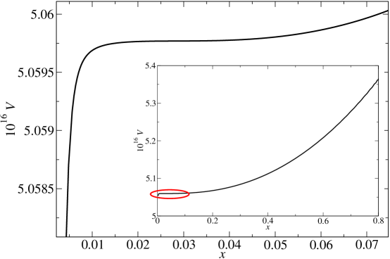
The shape of the potential is shown in Fig. 2, for the optimal parameter set (60) which will be discussed later. Away from the inflection point near $x=0.03$, it becomes steep, and starting from very large values of $x$ can lead to an overshoot of the flat region.

Figure 2: The potential for the optimal parameter set (60) (to be discussed later), in the vicinity of the inflection point. The inset shows the potential over a larger range of $x$.

III Equations of Motion

The kinetic term of the D3-brane comes from the Dirac-Born-Infeld (DBI) action, of the form $-a^{4}T_{3}\sqrt{1-a^{-4}\dot{X}^{2}}$, where $a$ is the warp factor in the throat. For small enough field velocities, we can expand to leading order in $\dot{X}^{2}$ to obtain a conventional kinetic term. We will check the validity of the approximation $a^{-4}\dot{X}^{2}\ll 1$ in our numerical analysis. In the framework of the low-energy supergravity effective action, the kinetic term for the D3-brane and the Kähler modulus comes with a nontrivial metric $G_{I\bar{J}}$ on the space of the complex fields, taking the form:

$${\cal L}_{\rm kin}=G_{I\overline{J}}\partial_{\mu}\Phi^{I}\partial^{\mu}{\overline{\Phi}}^{J}.$$ (21)

This leads to the kinetic term:

$${\cal L}_{\rm kin}={1\over a^{2}U^{2}}(3{\dot{\omega}}^{2}+2\omega_{0}\omega\phi_{\mu}^{2}{\dot{x}}^{2}).$$ (22)

We define the canonical momenta:

$$\pi_{x} \equiv {\partial{\cal L}\over\partial\dot{x}}=\frac{4\omega_{0}\omega\phi_{\mu}^{2}}{a^{2}U^{2}}\dot{x},$$ (23)

$$\pi_{\omega} \equiv {\partial{\cal L}\over\partial\dot{\omega}}=\frac{6}{a^{2}U^{2}}\dot{\omega},$$ (24)

which can be solved for the field velocities,

$$\dot{x} = \frac{a^{2}U^{2}}{4\omega_{0}\omega\phi_{\mu}^{2}}\pi_{x},$$ (25)

$$\dot{\omega} = {a^{2}U^{2}\over 6}\pi_{\omega}.$$ (26)

The equations of motion for the fields are

$$\dot{\pi}_{i}+3H\pi_{i} = {\partial\over\partial\phi_{i}}\left({\cal L}_{\rm kin}-V\right),\hskip 36.135pti=x,\omega,$$ (27)

$$3H^{2} = {\cal L}_{\rm kin}+V.$$ (28)

It is convenient to use the number of $e$-foldings instead of time as the independent variable:

$${d\over dt}=H{d\over dN}.$$ (29)

Then the equations of motion, in suitable form for numerical integration, are

$${d\pi_{x}\over dN} = -3\pi_{x}+{1\over H}\left(\frac{4\omega_{0}\phi_{\mu}^{2}x}{3aU}{\cal L}_{\rm kin}-{\partial V\over\partial x}\right),$$ (30)

$${d\pi_{\omega}\over dN} = -3\pi_{\omega}+{1\over H}\left(-{4\over aU}{\cal L}_{\rm kin}+\frac{2\omega_{0}\phi_{\mu}^{2}{\dot{x}}^{2}}{a^{2}U^{2}}-{\partial V\over\partial\omega}\right),$$ (31)

$${dx\over dN} = {1\over H}\dot{x},$$ (32)

$${d\omega\over dN} = {1\over H}\dot{\omega},$$ (33)

where $\dot{x}$ and $\dot{\omega}$ are determined through Eqs. (25) and (26); the derivatives of the potential are given in Appendix A.3.

In the regime that we are interested in, near the tip of the throat, $\omega\gg x$ and $\omega\simeq\omega_{0}$; then the equations of motion can be approximately written in canonical form Panda :

$${\cal L}_{\rm kin} = {1\over 2}{\dot{\phi}}^{2}+{1\over 2}{\dot{\chi}}^{2},$$ (34)

$$\ddot{\phi}+3H\dot{\phi} = -V_{\phi},$$ (35)

$$\ddot{\chi}+3H\dot{\chi} = -V_{\chi},$$ (36)

where

$$\chi=\sqrt{3\over 2}\ln\omega,$$ (37)

and $V_{X}$ denotes $\partial V/\partial X$. Although we will solve the exact equations of motion in this paper, the canonical fields are useful when discussing the primordial power spectrum and the spectral index, as will be seen in the following sections.

IV The Primordial Power Spectrum

The primordial power spectrum for single-field inflation is

$${\cal P_{R}}={H^{4}\over 4\pi^{2}{\dot{\phi}}^{2}}.$$ (38)

Generalizing to the noncanonical kinetic term, it can be written as Cline:2006hu

$${\cal P_{R}}={H^{4}\over 8\pi^{2}{\cal L}_{\rm kin}}.$$ (39)

The spectral index is

$$n_{s}\equiv 1+{d\ln{\cal P_{R}}\over d\ln k}=1+\left(4{d\ln H\over dN}-{d\ln{\cal L}_{\rm kin}\over dN}\right)\left(1+{d\ln H\over dN}\right)^{-1},$$ (40)

where $dH/dN$ and $d{\cal L}_{\rm kin}/dN$ can be calculated through the potential and its derivatives (see Appendix A.4 for details). Equation (39) is justified when there is effectively just a single field contributing (single direction in field space), since it is invariant under field redefinitions. However, it is not valid when the entropy perturbations make a significant contribution to the power spectrum.

The power spectrum and the spectral index can be expressed in terms of the slow-roll parameters by defining the adiabatic direction $\psi$ in field space, tangent to the inflaton trajectory Gordon:2000hv ,

$$\dot{\psi}=\dot{\phi}\cos\theta+\dot{\chi}\sin\theta,$$ (41)

where $\phi$ and $\chi$ are assumed to be canonically normalized, and

$$\cos\theta = {\dot{\phi}\over\sqrt{\dot{\phi}^{2}+\dot{\chi}^{2}}},$$ (42)

$$\sin\theta = {\dot{\chi}\over\sqrt{\dot{\phi}^{2}+\dot{\chi}^{2}}}.$$ (43)

If $\dot{\theta}\not=0$, then the trajectory is curved and entropy perturbations can source curvature perturbations on large scales ($k\to 0$). However if $\dot{\theta}$ is very small, or if the entropy mode is suppressed by large curvature of the potential in the direction orthogonal to $\psi$, which is the case in the present model Panda , the entropy mode can be ignored and then we have the usual formulas in terms of $\psi$,

$${\cal P_{R}} = {1\over 24\pi^{2}}{V\over\epsilon_{\psi}},$$ (44)

$$n_{s} = 1-6\epsilon_{\psi}+2\eta_{\psi\psi}.$$ (45)

The definitions of the slow-roll parameters are given in Appendix A.5. We will see that in the regime we are interested in, the slow-roll approximation is well satisfied, hence Eqs. (39) and (44) agree with each other.

V Tuning of Parameters

Using numerical integration and Monte Carlo techniques, we have undertaken a systematic study of the inflationary dynamics over the full parameter space of the model. In the following sections, we will first reproduce the known result Baumann ; Panda that, while keeping other parameters fixed, the tuning of the uplifting parameter $s$ allows one to obtain inflation with a sufficient number of $e$-foldings, $N\geq 50$. We then show that by varying the amplitude of the nonperturbative superpotential, $A_{0}$, one can satisfy both the COBE normalization and the WMAP constraint on the spectral index. (Recall that Ref. Panda claimed that it was difficult to satisfy both.) We next point out that the $s$ parameter is actually already fixed by the requirements of uplifting; however, there remains sufficient freedom to get a flat potential by varying $D_{01}$ and $\omega_{F}$.

V.1 Varying the tension to get flat potential

References Baumann ; Panda showed that by varying the value of $D_{0}$ (proportional to the warped D3-brane tension at the tip) one can obtain sufficiently many $e$-foldings of inflation. Here we further investigate the dependence of the potential on $s$, which is related to $D_{1}$ through Eq. (14), and fix other parameters as given in Ref. Baumann :

$$A_{0}=1,\ n=8,\ B_{4}=9.15,\ B_{6}=1.5,\ Q_{\mu}=1.2,\ N_{5}=32.$$ (46)

These values imply that

$$\phi_{\mu}=0.2406,\ \omega_{F}=10.009.$$ (47)

We set our new parameter $D_{01}$ to $1$ for the moment for definiteness. We use initial conditions:

$$x_{i}=0.8,\ \omega_{i}=\omega_{\ast}(x_{i}),\ \dot{x}_{i}=\dot{\omega}_{i}=0,$$ (48)

where $\omega_{\ast}$ is the instantaneous minimum which satisfies

$$\left.\frac{\partial V}{\partial\omega}\right|_{\omega_{\ast}=\omega_{\ast}(x)}=0.$$ (49)

The initial value $x_{i}=0.8$ is sufficient for getting inflation while avoiding the overshoot problem which we will discuss in Section VII.3. Taking the initial velocities to be zero is justified since any nonzero values would be quickly Hubble damped.

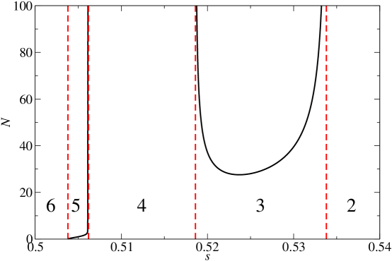
We now consider how the inflationary potential and the resulting solutions depend on $s$. Figure 3 shows the total number of $e$-foldings as a function of $s$. The parameter space of $s$ can be divided into six regions. They are

Figure 3: The total number of $e$-foldings versus the value of $s$. Dashed lines and numbers identify the regions described in the text.

1. $s>3.443$: $dV/d\omega\not=0$; there is no valley-shaped potential and no stable trajectory.

2. $0.5338<s\leq 3.443$: the inflaton gets trapped in a local minimum, $N\to\infty$.

3. $0.5186\leq s\leq 0.5338$: the potential is monotonic; for $s\to 0.5186$ or 0.5338, it is extremely flat and gives a large number of $e$-foldings.

4. $0.5062\leq s<0.5186$: the inflaton is again trapped in a local minimum, so $N\to\infty$.

5. $0.5038\leq s<0.5062$: there is a local minimum in the potential; however the inflaton has enough momentum to escape from it if slow roll had been attained earlier (e.g., starting with zero initial velocities $\dot{x}_{i}=\dot{\omega}_{i}=0$ at $x_{i}=0.8$).

6. $0<s<0.5038$: the potential is negative at $0<x<0.8$, so inflation ends in a big crunch.

We are interested in the cases where inflation will end (although not via a big crunch). Although region 5 allows for the inflaton to escape from the local minimum and end inflation, Fig. 3 shows that one needs to extremely fine-tune the value of $s$ to get enough $e$-foldings. Therefore we will focus on region 3, where the potential is monotonic, and much less tuning is needed. It is striking that there is a plateau in this region, signifying a minimum number of $e$-foldings of about 30. It is tempting to look for other parameters such that the minimum number of $e$-foldings of the plateau would be increased to more than 50. If that were possible, then one would say that inflation is generic rather than fine-tuned, at least with respect to the parameter $s$. To investigate this possibility, we need to search the multidimensional parameter space. This will be discussed in Section VI.

Region 3 is also the case that Ref. Panda focused on. The latter found that by adjusting the tension, one can have inflation with a correct spectral index and enough $e$-foldings, but they did not succeed in finding a model which satisfies the COBE normalization simultaneously. We confirm this: by restricting to the default parameters in Ref. Baumann and just varying the value of $s$, one cannot achieve $n_{s}\sim 0.96$ and ${\cal P_{R}}\sim 2.4\times 10^{-9}$ at $N\geq 50$.

V.2 Varying $A_{0}$: COBE normalization

Of course, by varying just one parameter, one should not expect to satisfy several experimental constraints. One usually realizes the COBE normalization by adjusting the overall scale of the potential. In Ref. Baumann , it was assumed that the prefactor $A_{0}$ played the role of the overall scale. However this is only true as long as the Coulombic interaction is negligible, because as shown in Eq. (14), $A_{0}$ is related to $D_{1}$ and hence contributes to the shape of the Coulomb interaction through Eq. (16). Therefore as long as $D_{01}>0$, which must be the case, $A_{0}$ does not merely determine the overall scale of the potential.

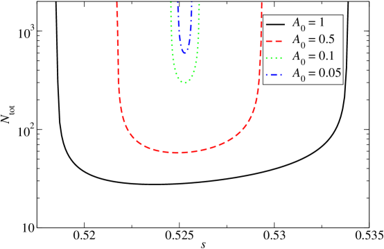
This can be seen explicitly by calculating the total number of $e$-foldings of inflation versus $s$ for varying values of $A_{0}$. If the shape of the potential did not depend on $A_{0}$, then the number of $e$-foldings would be completely insensitive to $A_{0}$, as long as the slow-roll approximation is valid. Figure 4 shows that in fact $N_{\rm tot}$ depends rather strongly on $A_{0}$: for smaller values of $A_{0}$ (closer to those needed for the COBE normalization), the range of $s$ values which give a monotonic potential becomes smaller. An interesting by-product is that the minimum number of $e$-foldings becomes bigger. This shows that when $A_{0}$ is adjusted to satisfy the COBE normalization, $s$ does not need to be fine-tuned to a special value to ensure that the number of $e$-foldings of inflation is sufficient. However, $s$ still needs to be within a narrow range to avoid the problem of the potential developing a local minimum in which the inflaton gets stuck, with no end to inflation. For example, taking $A_{0}=0.005$ and $s=0.5253$, we have ${\cal P_{R}}=2.41\times 10^{-9}$ at $N=73$ ($N_{\rm tot}\simeq 6000$), where $n_{s}=0.944$, within 2$\sigma$ of WMAP5’s result Komatsu:2008hk . We have an existence proof that it is possible to nearly satisfy all the cosmological constraints in the $D3$-$\overline{D3}$ inflation model; however this particular example appears to be fine-tuned. Below we will show that less fine-tuned examples can be found.

Figure 4: The total number of $e$-foldings versus the value of $s$ with different values of $A_{0}$.

V.3 Accounting for the uplifting constraint

Up to now we have regarded $s$ as a free parameter, as was done in the previous literature Baumann:2007np ; Baumann ; Panda . But as we have mentioned, $s$ should already be determined by the requirement of having vanishing cosmological constant at the end of inflation. In this section, we take this requirement into account and show that it is nevertheless still possible to tune to obtain a flat potential using the extra parameter $D_{01}$, which in fact has a similar qualitative effect to varying $s$.

First we show how the value of $s$ is fixed by setting

$$V(0,\omega_{0})=0.$$ (50)

Using Eq. (65), $\omega_{0}=\omega_{0}(s,\omega_{F})$, we find that

$$(2\omega_{F}+3)e^{\omega_{0}-\omega_{F}}-2\omega_{0}-5=0.$$ (51)

This shows that $\omega_{0}$ can be expressed as a function of $\omega_{F}$ only, $\omega_{0}=\omega_{0}(\omega_{F})$. From Eqs. (65) and (51), we have

$$s = \frac{\omega_{0}+2}{\omega_{F}}\left(\frac{2\omega_{F}+3}{2\omega_{0}+5}\right)^{2}$$ (52)

$$\simeq {\omega_{F}\over\omega_{0}}\left[1+3\left({1\over\omega_{F}}-{1\over\omega_{0}}\right)\right],$$ (53)

where the latter form assumes $\omega_{0}$, $\omega_{F}\gg 1$. Therefore, once $\omega_{F}$ is given, both $\omega_{0}$ and $s$ are fixed by uplifting $V(0,\omega_{0})=0$, and our use of $s$ to flatten the potential in the previous sections is seen to be invalid. For example, taking the value of $\omega_{F}$ in Eq. (47), we obtain $\omega_{0}=10.100,\ s=1.0087$.

To compensate for not being able to vary $s$, we can adjust the ratio of the tensions in the inflationary versus the other throats, i.e., $D_{01}$, while keeping $s$ fixed. We find that the qualitative dependence of the shape of the potential on $D_{01}$ is similar to the dependence on $s$. There are five regions of the $D_{01}$ parameter space which correspond to the first five enumerated for $s$ in Section V.1. The sixth region, where the potential became negative, no longer exists because we have now adjusted $s$ to avoid this problem. Furthermore, the dependence of the shape of the curves $N_{\rm tot}(D_{01})$ on the parameter $A_{0}$ is just like that for $N_{\rm tot}(s)$, as can be seen in Fig. 5. Again, as $A_{0}$ decreases, the minimum number of $e$-foldings of the plateau increases, while the monotonic region shrinks and more fine-tuning is needed.

Figure 5: The total number of $e$-foldings versus the value of $D_{01}$ with different values of $A_{0}$.

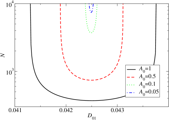
We find that varying only $(D_{01},A_{0})$ while keeping other parameters fixed is not sufficient for satisfying all the experimental constraints, but varying $(D_{01},\omega_{F})$ allows us to nearly do so. For example, taking $\omega_{F}=15$ and $D_{01}=0.1227$ gives ${\cal P_{R}}=2.41\times 10^{-9}$ and $n_{s}=0.949$ at $N=78$, out of the total number of $e$-foldings $N_{\rm tot}\simeq 10^{4}$. Generically we might have found that by varying two parameters, the two constraints ${\cal P_{R}}\sim 2.4\times 10^{-9}$ and $n_{s}\sim 0.96$ could be satisfied at the COBE scale, which we take to be $50\leq N_{e}\leq 60$. The fact that we cannot do so here is just due to unfortuitous values for some of the other parameters which are not varied. In the next section we will consider variations in the full parameter space, but here we are primarily concerned with the degree of fine-tuning needed to get sufficient inflation. The present example requires fine-tuning at the level of $0.13\%$ for $D_{01}$: the potential is monotonic from $D_{01}=0.122\,62$ to $0.122\,78$, so the relative fine-tuning is $1.6\times 10^{-4}/0.1227$, approximately 1 part in 1000. Below, we will identify other regions of parameter space where this problem is significantly alleviated.

VI Solving the Fine-Tuning Problem

Although the required values in the previous section may subjectively appear to be rather finely tuned, this is a notion which requires definition. One must distinguish fine-tuning from the more mundane necessity of fixing parameters to agree with experimental measurements. In this section we propose a measure on the volume of the experimentally allowed part of parameter space which will allow us to quantify the degree of fine-tuning needed in any localized region of the space. We calculate this statistic while doing a systematic search of the parameters. The results are described in the final part of this section, demonstrating that the fine-tuning problem is ameliorated for optimal values of the parameters.

Our goal now is to scan the parameter space in search of regions where less tuning is required. To make this quantitative, we need some specific measure of the degree of tuning, which varies locally in the parameter space. Suppose we have identified a set of parameters $p_{i}^{(0)}$ (where $i$ runs over the number of parameters) which satisfy some necessary criteria for inflation. We can then vary each parameter to find the maximum range $p_{i}^{(0)}-\sigma_{i}<p_{i}<p_{i}^{(0)}+\sigma_{i}$ for which these criteria are still satisfied. The width of this interval is $2\sigma_{i}$.

A first guess for a quantity which is anticorrelated with the degree of fine-tuning would be the volume in parameter space consistent with inflation, defined by the product of all the intervals $2\sigma_{i}$. The exact $N$-dimensional volume would be more complicated than our rectilinear approximation; we ignore this, and treat the $\sigma_{i}$’s as independent quantities, i.e., when determining $\sigma_{i}$, we fix other parameters at their central values, $p_{j}^{(0)}\ (i\not=j)$. The volume is thus given by

$$V_{N}\left(p_{i}^{(0)}\right)=2^{N}\prod_{i}\sigma_{i}.$$ (54)

However it would be naive to think that maximizing Eq. (54) corresponds to minimizing the tuning of parameters, because this would artificially reward parameter values that happen to be large in absolute terms. We are really interested in the relative variation of a given parameter. Therefore a better measure of naturalness is the relative volume,

$$\delta_{N}=\prod_{i}{2\sigma_{i}\over p_{i}^{(0)}}={V_{N}\over\prod\limits_{i}p_{i}^{(0)}}.$$ (55)

We can furthermore define a reduced relative volume,

$$\delta_{N}^{\prime}=\sqrt[N]{\delta_{N}},$$ (56)

whose reciprocal quantifies the average degree of tuning per parameter, and thus makes it meaningful to compare searches in which different numbers of parameters are varied.

VI.1 Description of algorithm

To explore the parameter space, we used the Metropolis algorithm, which looks for a function’s minimum by the method of simulated annealing nr . In our case, we chose the objective function $f_{\rm obj}$ to be the negative of the relative volume, Eq. (55). Because we are interested in the part of parameter space corresponding to Figs. 3 and 4, where there is always a minimum number of $e$-foldings of inflation, we chose as our criterion for successful inflation that the potential should be monotonic, rather than having a local minimum where inflation would never end. In addition, we want to select models that satisfy the experimental constraints. We do this by requiring that the central values $p_{i}^{(0)}$ of the regions correspond to experimentally allowed models, although we do not impose this additional requirement on the neighboring points that define the volume. Specifically, for the central point of each allowed volume we demand that the COBE normalization (${\cal P_{R}}=2.41\times 10^{-9}$) is satisfied with the number of $e$-foldings $50\leq N_{e}\leq 60$ before the end of inflation. We take this to be a reasonable reflection of uncertainties in the time of horizon crossing due to variations in the scale of inflation and reheat temperature. We also require the spectral index to be within 2$\sigma$ of the WMAP5 preferred value, $n_{s}=0.963\pm 0.028$ Komatsu:2008hk .

The motivation for measuring volumes which are consistent with inflation but not necessarily the particular experimental constraints we observe is the following. The volume of parameters satisfying some number of constraints would be a set of measure zero in the full parameter space. However we do not consider a model to be fine-tuned just because its parameters are fixed by certain measurements. Rather, it is the basic requirement of having a flat enough potential to get at least 60 $e$-foldings of inflation (and not getting stuck in a local minimum preventing an exit from inflation) which underlies the apparent need for tuning that we are interested in.

The actual objective function includes a few subtleties. For example, if a set of parameters does not give a monotonic potential nor satisfy the experimental constraints, then the relative volume can be defined to be zero. However, this gives no information to assist the Monte Carlo method in finding more favorable values since most points in the parameter space will have the same value of the objective function. In this case we therefore take the objective function (which is to be minimized) to be an empirical function of $N_{e}$, $\cal P_{R}$, and $n_{s}$:

$$f_{\rm obj}=\left\{\begin{array}[]{ll}f_{\rm emp}(N_{e},{\cal P_{R}},n_{s}),&\hskip 36.135pt\delta_{N}=0,\\ -\delta_{N},&\hskip 36.135pt\delta_{N}>0.\end{array}\right.$$ (57)

The empirical function is chosen in such a way as to help move the configuration from a nonmonotonic regime to a monotonic one, or from a regime not satisfying the experimental constraints to one which does. Once satisfactory parameters are found, then the relative volume is calculated, and maximizing $\delta_{N}$ leads to parameter values which are less fine-tuned.

The Metropolis algorithm uses an artificial temperature $T$ which randomly allows the objective function to sometimes increase rather than decrease; this is how it avoids getting stuck in a shallow local minimum rather than converging to some point closer to the global minimum. We used the downhill simplex method of Ref. nr as a generator of random steps, which moves the system’s configuration by reflections, expansions, and contractions in an $N$-dimensional simplex. As the temperature is lowered, the system relaxes to a minimum which should be close to the global minimum. During this iterative process, a chain of accepted parameter values is generated, which allows one to make statistical statements about the probabilities of the parameters.

VI.2 Monte Carlo results

Our starting point was the configuration given in the previous section, with the values

$$D_{01}=0.122\,70,\ \omega_{F}=15,\ A_{0}=1,\ \phi_{\mu}=0.240\,56,\ n=8.$$ (58)

Since we had not yet varied enough parameters, this does not quite satisfy all the experimental constraints: it has spectral index and normalization $n_{s}=0.949$ and ${\cal P_{R}}=2.41\times 10^{-9}$ at $N=78$ $e$-foldings before the end of inflation, instead of at the COBE scale. Nevertheless, since it is closer to the examples previously studied in the literature, we will use this as a reference point for comparison when assessing the improvement in fine-tuning. We also restarted the search using other initial conditions to avoid getting trapped in a local minimum. We accumulated approximately 200 chains containing more than 70 000 samples (each chain containing from 200 to 1000 samples). The control parameter $T$ was decreased by a factor $\epsilon$ after every $m$ moves, over several orders of magnitude (for example, changing from 100 to 0.001) during the entire simulated annealing process. The computing time for each chain can be as fast as five hours (on a PC), or as slow as ten days, depending on the configuration of the annealing schedule and the initial conditions.

To satisfy the experimental constraints we tried varying different combinations of the five independent parameters, $(D_{01},\omega_{F},A_{0},\phi_{\mu},n)$. Generically one would expect that any two parameters would be uniquely fixed by the two constraints; thus to obtain chains, one should vary at least three at a time. Indeed, we found that the combinations $(D_{01},\omega_{F},A_{0})$, $(D_{01},\omega_{F},\phi_{\mu})$, or $(D_{01},\omega_{F},n)$ were suitable for generating chains which evolved toward larger reduced volumes. In each case, the unvaried parameters take the values given in (58), which we refer to as the starting or fiducial point. The results are shown in Table 1, where it can be seen that the reduced volumes of parameter space grow to values of order unity, starting from very small initial values. This indicates that there is essentially no fine-tuning at the optimal points.

Table 1: The relative volumes and reduced volumes for different combinations of the parameters, showing initial and final values along the chains.

Parameters	Starting point		Optimal point
	$\delta_{3}$	$\delta_{3}^{\prime}$	$\delta_{3}$	$\delta_{3}^{\prime}$
$(D_{01},\omega_{F},A_{0})$	$9.0\times 10^{-7}$	0.96%	0.087	44%
$(D_{01},\omega_{F},\phi_{\mu})$	$5.2\times 10^{-10}$	0.080%	0.027	30%
$(D_{01},\omega_{F},n)$	$7.8\times 10^{-10}$	0.092%	0.020	27%

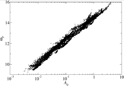
We can make more detailed statements about how the various parameters affect the power spectrum. For example, increasing $\omega_{F}$ has the effect of reducing the overall scale of the potential, due to the $e^{-2\omega}$ dependence, while increasing $A_{0}$ has the opposite effect. It is not surprising that the COBE normalization thus produces a strong correlation between $A_{0}$ and $\omega_{F}$ for the accepted parameter values, which can be seen in Fig. 6 (left panel). Also shown in that Fig. 6 (right panel) is the correlation of 4D relative volumes with the value of $\omega_{F}$ for the Monte Carlo chains. The latter demonstrates that larger values of $\omega_{F}$ are less likely than smaller ones, but only mildly so.

Figure 6: Left panel: scatter plot of accepted $\omega_{F}$ and $A_{0}$ values from search of 4D parameter space $(D_{01},\omega_{F},A_{0},\phi_{\mu})$. Right panel: correlation of $\delta_{4}$ and $\omega_{F}$.

Furthermore, we find a degeneracy between $\phi_{\mu}$ and $n$ on the shape of the potential: the effect of the discrete parameter $n$ (the number of D7-branes in the stack) can be compensated by changing the value of $\phi_{\mu}$. Therefore the subset $(D_{01},\omega_{F},A_{0},\phi_{\mu})$ gives an adequate representation of the possible potential shapes arising in the model. Fixing $n=8$ to eliminate the $\phi_{\mu}$-$n$ degeneracy, the Metropolis algorithm finds a global minimum of $f_{\rm obj}$, hence a maximum of the relative volume $\delta_{4}=0.052$. Table 2 compares the optimal point to the fiducial point given in the previous section for the 4D search. We see that the fiducial point required tuning at the level of $0.5$% per parameter; this number increases to 50% at the optimal point, so there is no more tuning. We also show the breakdown on a per-parameter basis: $2\sigma_{i}/p_{i}^{(0)}$ is the relative allowed width for the $i$th parameter. One might worry that the cruder statistic $\delta^{\prime}_{4}$ could hide severe tuning of some parameters by having very large values of $2\sigma_{i}/p_{i}^{(0)}$ for others, to which inflation happened to be insensitive. However we see from Table 2 that this is not the case: the most sensitive parameter is $D_{01}$, which is still only tuned at the 20% level, in the region of the optimal parameter values. The last row of the table shows that the tuning per parameter is ameliorated by at least a factor of 100 (except for $A_{0}$, which did not require fine-tuning even at the starting point).

Table 2: Comparison of parameter values and degree of fine-tuning between the fiducial (starting) point and the optimal point of 4D parameter search.

Configuration	$D_{01}$	$\omega_{F}$	$A_{0}$	$\phi_{\mu}$	$\delta_{4}$	$\delta_{4}^{\prime}$
Fiducial point	0.122 70	15	1	0.240 56	$4.5\times 10^{-10}$	0.46%
$2\sigma_{i}/p_{i}^{(0)}$	$1.3\times 10^{-3}$	$\ 8\times 10^{-4}$	0.86	$5\times 10^{-4}$	–	–
Optimal point	0.1976	9.550	0.007778	0.5894	0.052	48%
$2\sigma_{i}/p_{i}^{(0)}$	0.19	0.52	1.8	0.3	–	–
$\left[\sigma_{i}/p_{i}^{(0)}\right]_{\rm opt}$/$\left[\sigma_{i}/p_{i}^{(0)}\right]_{\rm fid}$	140	640	2.1	600	–	–

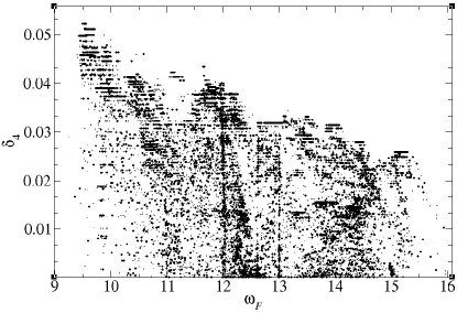
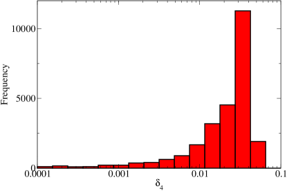
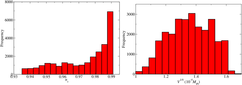
Given that points in our chains tend to accumulate where the relative volume is bigger and the tuning problem is less severe, we can use the chains to define a probability distribution on the space of parameters, as well as on the predictions of the model for observable quantities. The correlation between relatively large volume and high density of models can be seen in the distribution of $\delta_{4}$, Fig. 7. The distributions for the spectral index (within the $2\sigma$ range which we allowed around the WMAP5 central value) and the energy scale of inflation are shown in Fig. 8. We note there a preference for larger values of $n_{s}$ close to $0.99$, while $V_{\rm inf}^{1/4}$ is in the range $(1.1$-$1.6)\times 10^{-4}M_{\rm Pl}=(2.7$-$3.9)\times 10^{15}$ GeV.

Figure 7: Distribution of relative volume $\delta_{4}$ from the Monte Carlo chains. Notice the scale for $\delta_{4}$ is logarithmic.

Figure 8: Distribution of spectral index $n_{s}$ and inflationary scale, based on Monte Carlo chains.

VI.3 An alternative measure

Thus far, we have considered a well-defined and reasonable definition for the measure of fine-tuning on the parameter space: given a point which is consistent with the data, it measures the relative amount by which each parameter can be varied around this point and still be acceptable. However, one might argue that this hides fine-tuning problems in the case where the central values are orders of magnitude smaller than the largest theoretically allowed values (similar to the cosmological constant problem). In this section, we therefore consider an alternative measure, which is the absolute volume of parameter space consistent with measurements, Eq. (54), instead of the relative volume.

The absolute parameter volume as a measure of fine-tuning has some conceptual difficulties which are not present in the relative volume measure. First, it is possible that some parameters have a formally infinite range, such as the Kähler modulus $\omega_{F}$. One has to regularize this divergence in order to make any sensible statements about probability. Second, we must disentangle the issue of fixing parameter values through measurements from that of fine-tuning. For example, in the theory of quantum electrodynamics, we do not say that the charge of the electron is fine-tuned just because its value is experimentally known to a very high precision. The tuning problem we are concerned with is one where different free parameters have to be adjusted with respect to each other to a high precision in some artificial way that had no a priori justification. Thus to implement the absolute volume measure, it makes sense to consider the volume only of some linear combinations of parameters which are not fixed by experimental constraints. This has the added advantage of possibly solving the first problem: we can use the experimental constraints to fix values of parameters which have no theoretical upper bound.

There is a further shortcoming in the absolute volume measure when degeneracies exist between parameters. In the present case, the scale of the inflaton potential is determined by the product of two prefactors, $A_{0}^{2}$ and $e^{-2\omega_{F}}$. As a result, a degeneracy between $\ln A_{0}$ and $\omega_{F}$ exists, as is confirmed by Fig. 6 (left panel). One can achieve a large absolute volume by trading $\omega_{F}$ for $A_{0}$. For instance, we find models with super-Planckian values of $A_{0}$ of order $O(10^{6})$ ($\omega_{F}\simeq 30$) having $\sigma_{A_{0}}\sim O(10^{6})$ and $V_{4}\sim O(10^{4})$, whereas the absolute volume near the fiducial point is $2\times 10^{-10}$; see Table 3. But it would be misleading to claim that the model $(\omega_{F},A_{0})\sim(30,10^{6})$ has less fine-tuning than that with $(\omega_{F},A_{0})\sim(10,0.01)$, because the large $V_{4}$ is a result of the fact that the potential has different sensitivities to $\omega_{F}$ and $A_{0}$. The relative volume, on the other hand, can balance the different sensitivities between different parameters.

Despite these complications, it might still be of interest to know the ratio of the allowed volume to the total volume of the parameter space,

$$\Delta_{N}=\frac{V_{N}}{\prod\limits_{i}p_{i,{\rm max}}},$$ (59)

where $p_{i,{\rm max}}$ denotes the theoretical maximum of the parameter. As mentioned above, $\omega_{F}$ has no maximum value, and the same is true of $D_{01,{\rm max}}$. Before dealing with this, let us consider just the numerator in (59), $V_{N}$ itself. We have repeated the Monte Carlo search of parameter space to find regions where $V_{N}$ are maximized. The results are shown in Table 3. There it can be seen that while $V_{N}$ is only $2\times 10^{-10}$ for the fiducial (starting) point, it increases to $0.03$ at the optimal point, which is different from the optimal point for the relative volume shown in Table 2. It is interesting that the improvement, 8 orders of magnitude, is the same as we obtained using the relative volume as the measure. Our conclusion that the degree of delicateness depends on the parameter values, and is greatly ameliorated in some regions of parameter space compared to others, thus holds for both the relative volume measure and the absolute volume measure.

Table 3: Comparison of parameter values and absolute allowed volume between the fiducial (starting) point and the optimal point of 4D parameter search.

Configuration	$D_{01}$	$\omega_{F}$	$A_{0}$	$\phi_{\mu}$	$V_{4}$
Fiducial point	0.122 70	15	1	0.240 56	$2\times 10^{-10}$
$2\sigma_{i}$	$1.6\times 10^{-4}$	0.012	0.86	$1.2\times 10^{-4}$	–
Optimal point	0.2186	13.70	0.6341	0.4383	0.03
$2\sigma_{i}$	0.06	11	0.73	0.063	–
$\left[\sigma_{i}\right]_{\rm opt}$/$\left[\sigma_{i}\right]_{\rm fid}$	380	920	0.85	530	–

Although the optimal case is much less fine-tuned than the fiducial point, we are still left with the question of how fine-tuned is it in an absolute sense, which would be answered if $\Delta_{N}$ was well defined. If we adopt the approach suggested above, of eliminating the parameters which have no maximum value ($\omega_{F}$ and $D_{01}$), then we are left with $\Delta_{2}$ for the remaining parameters $A_{0}$ and $\phi_{\mu}$. The maximum value of $\phi_{\mu}$ is 1, the maximum initial separation between the D3-branes and anti-D3-branes; similarly, $A_{0}$ should be less than the Planck scale due to gaugino condensation. This gives $\Delta_{2}=0.046$ and $\sqrt{\Delta_{2}}=0.2$ for the mean degree of tuning per parameter. This is comparable to the result we obtained using the relative volume measure.

Alternatively, instead of eliminating the $D_{01}$ and $\omega_{F}$ parameters, we could compare their widths to some “reasonable” or “generic” values. Since $D_{01}$ is the ratio of two brane tensions, $D_{01}\sim 1$ would seem to be a generic value. As for $\omega_{F}$, even though in principle it could be arbitrarily large, in practice it is difficult to make it very large. It is a derived parameter, which depends upon $W_{0}$ through Eq. (12). For example, if $W_{0,{\rm min}}\sim 10^{-42}$, then $\omega_{F,{\rm max}}\sim 100$. We see that in fact it requires a high degree of fine-tuning of $W_{0}$ to make $\omega_{F}$ very large. Generously taking 100 to be its maximum value (even though this would be considered unreasonably large by most string theorists), we then find that $\Delta_{4}=3\times 10^{-4}$, $\sqrt[4]{\Delta}_{4}\sim 0.1$, again a quite modest level of tuning per parameter.

VII Properties of the Optimal Parameter Set

Having identified a favorable region in the space of the model parameters, we now consider a number of its detailed properties, including its consistency with string theoretic constraints, the shape of the inflationary trajectory, and sensitivity to initial conditions and the overshoot problem. We also explain a potential subtlety concerning the computation of the spectral index in the single-field approximation to the model.

VII.1 Microscopic parameter values

The parameters ($D_{01},\omega_{F},A_{0},\phi_{\mu}$) which were convenient to vary in the potential are not all fundamental from the string theoretic point of view. We would like to determine the values of the microscopic stringy parameters which are compatible with the optimal point in Table 2, which has

$$D_{01}=0.1976,\quad\omega_{F}=9.550,\quad A_{0}=0.007\,778,\quad\phi_{\mu}=0.5894,\quad n=8.$$ (60)

These yield the derived parameters $\omega_{0}=9.644$, $s=1.0094$, and the corresponding observational predictions are ${\cal P_{R}}=2.41\times 10^{-9}$ for the primordial power spectrum and $n_{s}=0.989$ for the spectral index, at $N=52$ $e$-foldings before the end of inflation, out of a total of $N_{\rm tot}=134$ $e$-foldings of inflation. It is straightforward to find a reasonable set of stringy parameters $(N_{5},B_{4},B_{6},Q_{\mu})$ giving the desired $(\phi_{\mu},\omega_{F})$. For example, taking $Q_{\mu}=1.07$ and $N_{5}=10$, we need $B_{4}=75.28$, $B_{6}=1.0058$. This set satisfies all the microscopic consistency conditions in Appendix A.2.

One might however be concerned that such a small value of $\omega_{F}$ as 9.6 is only marginally consistent with the need for control over higher derivative corrections to the low-energy effective action, which are suppressed by the large compactification volume (hence small curvatures). Figure 6 shows that larger values of $\omega_{F}$ are indeed possible, up to a maximum of $\omega_{F}\simeq 15$; beyond this point, overly large values of $A_{0}>1$ would have to compensate the reduction in the inflationary scale needed to get the right COBE normalization. Thus one can increase $\omega_{F}$ to somewhat larger values, but at the expense of saturating the consistency condition $A_{0}<1$, and somewhat increasing the degree of fine-tuning. However at $\omega_{F}\simeq 14.5$, where the constraint $A_{0}<1$ starts to become important, there is actually no fine-tuning: the reduced volume becomes $\delta_{4}\simeq 0.021$ at this point, as opposed to the optimal value $\delta_{4}\simeq 0.052$. (Recall that $\delta_{4}^{\prime}=\sqrt[4]{\delta_{4}}=38$% quantifies the degree of tuning per parameter.)

VII.2 Taylor expansion of DBI kinetic term

Another point of consistency concerns the expansion of the DBI action for the inflaton kinetic term $-a^{4}T_{3}\sqrt{1-a^{-4}\dot{X}^{2}}$ where $T_{3}=m_{s}^{4}/(8\pi^{3}g_{s})$ is the 3-brane tension and $a$ is the warp factor in the throat. Notice that the canonically normalized inflaton field is $\phi\sim\sqrt{T_{3}}X$ after Taylor expanding this expression. Estimating the inflation scale as $V_{\rm inf}^{1/4}\sim am_{s}$, we see that the criterion for being able to safely expand the DBI action into standard form is $\dot{\phi}^{2}\ll T_{3}a^{4}=V_{\rm inf}/(8\pi^{3}g_{s})$. On the other hand, the slow-roll equation of motion gives $3H\dot{\phi}\simeq-V_{\phi}$. Since $3H^{2}\simeq V_{\rm inf}$, this condition can thus be rewritten in terms of the slow-roll parameter $\epsilon=\frac{1}{2}(V_{\phi}/V)^{2}$, as

$$\epsilon\ll{3\over{16\pi^{3}g_{s}}}.$$ (61)

This is clearly satisfied in the present model, since as we will show, $\epsilon\simeq 10^{-9}$ at the horizon crossing.

VII.3 Initial conditions

A potentially problematic aspect of the model is the need for special initial conditions, even if the potential itself is not finely tuned. Obviously, inflation takes place near the inflection point of the potential, so $\phi$ must not start lower than this point. But as was pointed out in Ref. Underwood:2008dh , $\phi$ also should not start too much above the inflection point, because of the overshoot problem: the inflaton can gain so much speed that it quickly rolls past the inflection point without ever rolling slowly. For the optimal parameter set we consider, however, there is another consideration which prevents us from exploring the regime where overshoot would take place. This is because of the angular directions of the extra dimensions in the throat, which we have set to the values which minimize their potential. As shown in Ref. Baumann , the positions of the angular minima flip when $\phi$ exceeds a certain critical value $\phi_{\rm c}$, given by Eq. (C.24) of that paper. We would need to follow all the angular fields as well to investigate this regime quantitatively, which is beyond the scope of the present work. If the potential is assumed to have the same form for $\phi>\phi_{\rm c}$, we do observe overshooting, starting from initial conditions of order $10\phi_{\rm c}$, but since we do not trust the potential in this regime, no reliable statement about overshooting can be made in the present context.

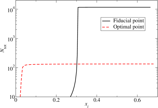
Nevertheless, we can quantify the range of initial conditions over which we get sufficient inflation and the potential is also valid: the allowed initial separation of the branes is $x=0.301\to 0.665$ for the fiducial point, while it is $x=0.029\to 0.680$ for the optimal point. We see that the allowed field range is expanded by a factor of 2 in the optimal case. Figure 9 shows the total number of $e$-foldings as a function of the initial conditions in these two cases. In an upcoming paper UC , we will give a more satisfactory solution to the problem of initial conditions in this model, based on the idea of Ref. CS .

Figure 9: The total number of $e$-foldings as a function of the initial condition $x_{i}$. The solid curve is for the fiducial parameters (58), the dashed curve is for the optimal ones (60).

VII.4 One field versus two: the spectral index

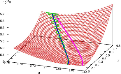
The present model has only one flat direction, so it is effectively a single-field inflation model. However, there is significant bending in the field space of $\omega$ and $\phi$, as illustrated in Fig. 10. In the left panel of Fig. 10, the solid, smooth, leftmost curve is the “instantaneous minimum” $\omega_{\ast}(x)$, defined in Eq. (49), while the wavy curve is the actual trajectory found by solving the equations of motion, given some initial displacement of the heavy field $\omega$ away from its instantaneous minimum. We used the initial condition $\omega_{i}=\omega_{\ast}(x_{i})+0.01$, so there are oscillations at first which allow one to distinguish the two curves. The solid curve on the right is the effective single-field description given by Refs. Baumann:2007np ; Baumann :

$$\omega\simeq\omega_{0}\left[1+{1\over n\omega_{F}}\left(1-{1\over 2\omega_{F}}\right)x^{3/2}\right].$$ (62)

As can be seen from the figure, it is not a very good approximation. Panda et al. Panda argued that using Eq. (62) underestimates the total number of $e$-foldings by an order of magnitude. However, this does not invalidate the single-field description; the real instantaneous minimum $\omega_{\ast}(x)$ does give a good approximation to the actual trajectory, once the oscillations have Hubble damped away.

Figure 10: Left panel: actual inflationary trajectories in the valley-shaped potential, and a plot of approximate trajectory Eq. (62). Right panel: projection of the same trajectories onto the $\omega$-$x$ plane.

However a subtlety can arise in the computation of the spectral index when we use the slow-roll approximation (45). The slow-roll parameters along the adiabatic direction $\psi$ are related to those along the component field directions $\phi\equiv\phi_{\mu}x$ and $\chi\equiv\sqrt{3/2}\ln\omega$ by Eqs. (88) and (89) which we repeat here for convenience:

$$\epsilon_{\psi}\simeq\epsilon_{\phi}+\epsilon_{\chi},\quad\eta_{\psi\psi}\simeq{1\over\epsilon_{\phi}+\epsilon_{\chi}}\left(\epsilon_{\phi}\eta_{\phi\phi}+\epsilon_{\chi}\eta_{\chi\chi}+{V_{\phi}V_{\chi}\over V^{2}}\eta_{\phi\chi}\right).$$ (63)

The problem occurs if we try to use these expressions to compute the spectral index $n_{s}$ by assuming the inflaton rolls exactly along the instantaneous minimum $\omega=\omega_{*}(x)$. By definition, $\epsilon_{\chi}=\epsilon_{\omega}=0$ along this trajectory. However, if we neglect the terms proportional to $\epsilon_{\chi}$ in $\eta_{\psi\psi}$, we get a result which does not agree with computing the spectral index directly from $d\ln P/d\ln k$, Eq. (40).

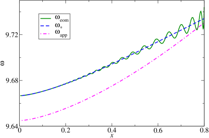
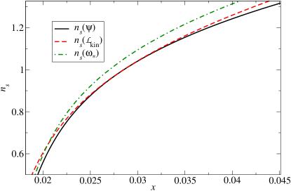
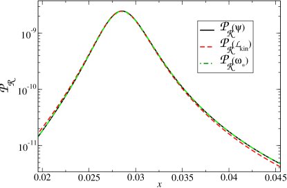
These conflicting results can be seen as the topmost (dot-dashed) and middle (dashed) curves, respectively, of Fig. 11 (left panel), labeled as $n_{s}(\omega_{*})$ and $n_{s}({\cal L}_{\rm kin})$. The latter is based upon the approximation (39) for the power spectrum, and since it comes from directly differentiating ${\cal P_{R}}(k)$, it must be the correct result. The curve $n_{s}(\omega_{*})$ significantly overestimates the spectral index as $n_{s}=1.065$ near the inflection point ($x=0.029$), whereas the correct value is $n_{s}=0.989$ for this example. Three approximations for the power spectrum itself, as a function of inflaton position $x$, are shown in the right panel of Fig. 11: ${\cal P}_{\cal R}(\psi)$, based on the slow-roll approximation (44), ${\cal P}_{\cal R}({\cal L}_{\rm kin})$ using (39) along the exact trajectory, and ${\cal P}_{\cal R}(\omega_{*})$ using (44) along the instantaneous minimum $\omega=\omega_{*}(x)$. It can be seen that they all agree quite well with each other near the inflection point, showing that $\omega=\omega_{*}(x)$ is indeed a good approximation.

Figure 11: Left panel: three approximations (described in the text) for the spectral index as a function of inflaton position $x$, indicating a problem with the slow-roll approximation on the instantaneous minimum trajectory, labeled $n_{s}(\omega_{\ast})$. Right panel: three approximations for the power spectrum as a function of $x$ (see text).

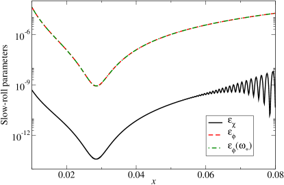
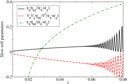
Nevertheless, the resolution of the problem is that the actual inflaton trajectory does not exactly follow the instantaneous minimum $\omega=\omega_{*}(x)$; it deviates slightly from this, like a race car on a banked curve. Therefore $\epsilon_{\chi}\neq 0$ on the true trajectory (although it is much smaller than $\epsilon_{\phi}$), as plotted in the left panel of Fig. 12, and the two terms $\epsilon_{\chi}\eta_{\chi\chi}$ and $V_{\phi}V_{\chi}\eta_{\phi\chi}/V^{2}$ make an important contribution to $\eta_{\psi\psi}$. In fact, the right panel of Fig. 12 shows that these two terms very nearly cancel $\epsilon_{\phi}\eta_{\phi\phi}$ ($1-n_{s}=0.011$). The spectral index evaluated along the actual trajectory, but using the slow-roll formula (45), is denoted $n_{s}(\psi)$. Figure 11 shows that it gives a good fit to the numerically computed index $n_{s}({\cal L}_{\rm kin})$ in the most important region, where most of inflation is taking place. Therefore the two-field slow-roll formula for $n_{s}$ is a good approximation, but only if one uses the correct two-field trajectory and not the instantaneous minimum approximation.

Figure 12: Left panel: the slow-roll parameters $\epsilon_{\phi}$ and $\epsilon_{\chi}$. $\epsilon_{\phi}$ is shown for both the exact trajectory and the approximation $\omega=\omega_{*}(x)$. Notice that $\epsilon_{\chi}=0$ in that approximation, so $\epsilon_{\chi}$ is only shown for the exact trajectory. Right panel: the three terms which contribute to $\eta_{\psi\psi}$ in Eq. (63).

VIII Conclusions

In this paper we have made a detailed study of the warped $D3$-$\overline{D3}$ inflation model, accounting for superpotential corrections, from a phenomenological perspective, but also with attention to the need for self-consistency from the string theoretical point of view. We extended the model slightly by including uplifting from throats other than the inflationary one, which was necessary so that inflation could end with a nearly vanishing cosmological constant. We subsequently explored the parameter space using Monte Carlo methods, finding for the first time values which satisfy all theoretical and experimental constraints. Moreover we identified an optimal set of parameters in the vicinity of which there appears to be no need for fine-tuning. This arises in part because of a peculiar feature of the potential in this model: there are ranges of the parameter $D_{01}$ for which one finds a minimum number of $e$-foldings of inflation, because at the boundaries of such regions, a local minimum develops, giving rise to $N_{\rm tot}\to\infty$. Toward this end, we defined the concept of a relative volume $\delta_{N}$ in an $N$-dimensional parameter space consistent with successful inflation, and having the property that $\sqrt[N]{\delta_{N}}$ represents the average degree of fine-tuning of any parameter. We obtained an improvement by 8 orders of magnitude in $\delta_{4}$ for the 4-parameter subspace which was needed to fully describe the range of potential shapes in the model, relative to the fine-tuned example from the literature with which we started our Monte Carlo search. We conclude that this string theoretic inflation model is not as delicate as it first seemed in Ref. Baumann:2007np .

There are some caveats to this successful conclusion however. The value of the Kähler modulus at the optimal point, $\omega_{F}=9.6$, is only marginally large enough to give one confidence that the low-energy effective field theory is not significantly perturbed by higher dimensional operators (coming from integrating out the extra dimensions) which are supposed to be suppressed by large $\omega_{F}$. On the other hand, since the scale of the potential goes like $e^{-2\omega_{F}}A_{0}^{2}/M_{\rm Pl}^{2}$, the COBE normalization demands that increasing $\omega_{F}$ must be accompanied by an exponential increase in $A_{0}$. The latter is related to the energy scale $\Lambda$ of gaugino condensation (or a Euclidean D3-brane) by $A\sim\Lambda^{3}$, which should certainly not exceed the Planck scale, and likely should also lie below the warped string scale. This could be a source of theoretical tension for the model.

On the phenomenological side, since we allowed for 2$\sigma$ deviations of $n_{s}$ from the WMAP5 central value in our Monte Carlo search, we can detect a statistical preference of the model for larger values of $n_{s}$ near $0.99$. That is to say, the least fine-tuned models which we find correspond to such higher values of $n_{s}$, and therefore if future data are shown to prefer lower values, it would be an indication disfavoring the model. In this way, our global search of the parameter space helps to provide an additional predictive tool which would not be available by simply finding a few sets of parameter values which were consistent with the data. This statement assumes that there is a landscape of string vacua which allows for nature to scan through the possible values of the parameters.

We also investigated an alternative measure of the degree of fine-tuning, i.e., the absolute allowed volume. While the motivation for this measure is different from that of the relative measure, the result is nearly the same—we found regions in the parameter space where the absolute allowed volume is increased by 8 orders of magnitude, and the overall degree of tuning per parameter is still at the 10% level. This finding reinforces our point that parameter regions exist where the severity of fine-tuning is greatly ameliorated.

Note added. While we were finishing this work, Ref. Kachru appeared, where it was pointed out that generic deformations of the throat geometry can have a qualitatively similar effect to the superpotential corrections, in allowing for an inflection point in the potential. More recently Ref.  Ali appeared, which reaches a different conclusion than ours, finding too large a value of $n_{s}$. Their work starts with a somewhat different model, based on the deformations discussed in Ref. Kachru rather than superpotential corrections. But since the latter model is supposed to have qualitatively similar behavior to the former, the result of Ref. Ali looks surprising. This discrepancy comes from the neglect of the Coulomb interaction in Ref. Ali . We thank the authors of Ref. Baumann for clarifying this point for us.

Appendix A Equations

Here we compile various formulas needed in the previous sections.

A.1 $\omega_{\ast}(x)$ and $\omega_{0}$

The instantaneous minimum $\omega_{\ast}(x)$ is defined through Eq. (49). This leads to the result

$$2s\omega_{F}e^{2\omega_{\ast}-2\omega_{F}}g^{-2/n}\left(1+\frac{D_{01}}{1+C_{D}\displaystyle{D_{0}\over x^{4}}}\right)-(2\omega_{F}+3)\left(2+\omega_{\ast}-{1\over 6}\omega_{0}\phi_{\mu}^{2}x^{2}\right)e^{\omega_{\ast}-\omega_{F}}g^{-1/n}$$

$$+2\omega_{\ast}^{2}+\left[7-{1\over 3}\omega_{0}\phi_{\mu}^{2}x^{2}+{3\over ng}\left({cx\over g}-x^{3/2}\right)\right]\omega_{\ast}+{3\over ng}\left({cx\over g}-x^{3/2}\right)\left(1-{1\over 6}\omega_{0}\phi_{\mu}^{2}x^{2}\right)$$

$$-{5\over 6}\omega_{0}\phi_{\mu}^{2}x^{2}+6=0.$$ (64)

Setting $x=0$, we have the equation for $\omega_{0}=\omega_{0}(s,\omega_{F})$:

$$2s\omega_{F}e^{2\omega_{0}-2\omega_{F}}-(2\omega_{F}+3)(2+\omega_{0})e^{\omega_{0}-\omega_{F}}+2\omega_{0}^{2}+7\omega_{0}+6=0.$$ (65)

This equation generically has two solutions for $\omega_{0}$; the one closest to $\omega_{F}$ is the minimum while the one farther from $\omega_{F}$ is at the maximum of the potential.

If we apply the uplifting condition, $V(0,\omega_{0})=0$, then the parameter $s$ is fixed and $\omega_{0}$ is a function of $\omega_{F}$ only; see Section V.3.

A.2 Microscopic constraints on the parameters

There is a constraint on the allowed field range of the inflaton field Baumann :

$$\Delta\phi<{2\over\sqrt{N_{5}}}.$$ (66)

If we consider $0<x<1$ only, then the parametrization Eq. (19) requires $B_{6}>1$ and $Q_{\mu}>1$. It is also required that $B_{4}>1.$ To satisfy the COBE normalization, one requires $\omega_{0}<O(30)$; otherwise the inflation scale will be too low. Using the fact that $\omega_{F}\simeq\omega_{0}$ leads to the further constraint ${N_{5}/n}<O(10^{2})$.

A.3 Potential and its derivatives

We rewrite the potential as

$$V=V_{F}+V_{D}\equiv{a|A_{0}|^{2}\over 3U^{2}}(V_{f}+V_{d}),$$ (67)

where

$$V_{f} = e^{-2\omega}g^{2/n}\left[2\omega+6-2(2\omega_{F}+3)e^{\omega-\omega_{F}}g^{-1/n}+{3\over ng}\left({cx\over g}-x^{3/2}\right)\right],$$ (68)

$$V_{d} = 2s\omega_{F}e^{-2\omega_{F}}\left(1+\frac{D_{01}}{1+C_{D}\displaystyle{D_{0}\over x^{4}}}\right).$$ (69)

Then we have

$${\partial V\over\partial\omega} = {a|A_{0}|^{2}\over 3U^{2}}\left\{-{4(V_{f}+V_{d})\over aU}-2V_{f}+2\left[1-(2\omega_{F}+3)e^{\omega-\omega_{F}}g^{-1/n}\right]e^{-2\omega}g^{2/n}\right\},$$ (70)

$${\partial V\over\partial x} = {a|A_{0}|^{2}\over 3U^{2}}\left[{4\omega_{0}\phi_{\mu}^{2}x\over 3aU}(V_{f}+V_{d})+{\partial V_{f}\over\partial x}+{\partial V_{d}\over\partial x}\right],$$ (71)

where

$${\partial V_{f}\over\partial x} = {3\over ng}\left\{\sqrt{x}V_{f}+e^{-2\omega}g^{2/n}\left[\sqrt{x}(2\omega_{F}+3)e^{\omega-\omega_{F}}g^{-1/n}-{3\sqrt{x}\over g}\left({1\over 2}+{cx\over g}\right)+{c\over g}\right]\right\},$$ (72)

$${\partial V_{d}\over\partial x} = 8s\omega_{F}e^{-2\omega_{F}}C_{D}D_{1}D_{01}^{2}x^{-5}\left(1+{C_{D}D_{0}\over x^{4}}\right)^{-2}.$$ (73)

We need the second order derivatives when calculating the slow-roll parameters:

$${\partial^{2}V\over\partial\omega^{2}} = -{8\over aU}\left({V\over aU}+{\partial V\over\partial\omega}\right)+{2a|A_{0}|^{2}\over 3U^{2}}\left\{2V_{f}+e^{-2\omega}g^{2/n}\left[-4+3(2\omega_{F}+3)e^{\omega-\omega_{F}}g^{-1/n}\right]\right\},$$

$${\partial^{2}V\over\partial x^{2}} = {4\omega_{0}\phi_{\mu}^{2}\over 3aU}\left(V+2x{\partial V\over\partial x}-{2\omega_{0}\phi_{\mu}^{2}x^{2}\over 3aU}V\right)+{a|A_{0}|^{2}\over 3U^{2}}\left({\partial^{2}V_{f}\over\partial x^{2}}+{\partial^{2}V_{d}\over\partial x^{2}}\right),$$ (75)

where

$${\partial^{2}V_{f}\over\partial x^{2}} = {3\sqrt{x}\over ng}\left\{\left({1\over 2x}-{3\sqrt{x}\over ng}\right)V_{f}+\left(2-{n\over 2}\right){\partial V_{f}\over\partial x}+e^{-2\omega}g^{2/n}\left[(2\omega_{F}+3)e^{\omega-\omega_{F}}g^{-1/n}\right.\right.$$ (76)

$$\left.\left.\times\left({1\over 2x}-{3\sqrt{x}\over 2ng}\right)+{3\over 2g}\left({6cx^{3/2}\over g^{2}}+{3\sqrt{x}\over 2g}-{3c\over g}-{1\over 2x}\right)-{3c\over 2g^{2}}\right]\right\},$$

$${\partial^{2}V_{d}\over\partial x^{2}} = -40s\omega_{F}{\rm e}^{-2\omega_{F}}C_{D}D_{1}D_{01}^{2}x^{-6}\left(1+{C_{D}D_{0}\over x^{4}}\right)^{\!\!-2}\!\left[1-{8C_{D}D_{0}\over 5x^{4}}\left(1+{C_{D}D_{0}\over x^{4}}\right)^{-1}\right],$$ (77)

and

$${\partial^{2}V\over\partial x\partial\omega} = {4\omega_{0}\phi_{\mu}^{2}x\over 3aU}\left[2\left(1+{1\over aU}\right)V+{\partial V\over\partial\omega}\right]-2\left(1+{2\over aU}\right){\partial V\over\partial x}$$ (78)

$$+{2a|A_{0}|^{2}\over 3U^{2}}\left\{{\partial V_{d}\over\partial x}+{3\sqrt{x}\over 2ng}e^{-2\omega}g^{2/n}\left[2-(2\omega_{F}+3)e^{\omega-\omega_{F}}g^{-1/n}\right]\right\}.$$

A.4 Power spectrum

The kinetic part of the Lagrangian is

$${\cal L}_{\rm kin}={a^{2}U^{2}\over 4}\left({1\over 3}\pi_{\omega}^{2}+\frac{\pi_{x}^{2}}{2\omega_{0}\omega\phi_{\mu}^{2}}\right).$$ (79)

Its derivative is given by

$$\frac{d{\cal L}_{\rm kin}}{dN}={4{\cal L}_{\rm kin}\over aU}\left({d\omega\over dN}-{\omega_{0}\phi_{\mu}^{2}x\over 3}{dx\over dN}\right)+{a^{2}U^{2}\over 4}\left[{2\pi_{\omega}\over 3}{d\pi_{\omega}\over dN}+\frac{\pi_{x}}{\omega_{0}\omega\phi_{\mu}^{2}}\left({d\pi_{x}\over dN}-{\pi_{x}\over 2\omega}{d\omega\over dN}\right)\right],$$ (80)

where $dx/dN$, $d\omega/dN$, $d\pi_{x}/dN$, and $d\pi_{\omega}/dN$ are obtained by solving the equations of motion. From Eq. (28), we have

$${d\ln H\over dN}={1\over 6H^{2}}\left({d{\cal L}_{\rm kin}\over dN}+V_{x}{dx\over dN}+V_{\omega}{d\omega\over dN}\right).$$ (81)

The spectral index can be calculated through Eq. (40).

A.5 Slow-roll parameters

The slow-roll parameters for a generic field $\phi$ are defined as

$$\epsilon_{\phi} = {1\over 2}\left({V_{\phi}\over V}\right)^{2},$$ (82)

$$\eta_{\phi\phi} = {V_{\phi\phi}\over V},$$ (83)

where $V_{\phi\phi}\equiv{\partial^{2}V/\partial\phi^{2}}$. Since Gordon:2000hv

$$V_{\psi} = V_{\phi}\cos\theta+V_{\chi}\sin\theta,$$ (84)

$$V_{\psi\psi} = V_{\phi\phi}\cos^{2}\theta+V_{\chi\chi}\sin^{2}\theta+V_{\phi\chi}\sin 2\theta,$$ (85)

we have

$$\epsilon_{\psi} = {1\over\dot{\phi}^{2}+\dot{\chi}^{2}}\left(\dot{\phi}^{2}\epsilon_{\phi}+\dot{\chi}^{2}\epsilon_{\chi}+\dot{\phi}\dot{\chi}{V_{\phi}V_{\chi}\over V^{2}}\right),$$ (86)

$$\eta_{\psi\psi} = {1\over\dot{\phi}^{2}+\dot{\chi}^{2}}\left(\dot{\phi}^{2}\eta_{\phi\phi}+\dot{\chi}^{2}\eta_{\chi\chi}+2\dot{\phi}\dot{\chi}\eta_{\phi\chi}\right).$$ (87)

In general, one should not apply the slow-roll approximation to all the terms in these expressions since one linear combination of the fields is heavy. However, we are interested in trajectories along the flat direction of the potential, after any oscillations in the steep directions have Hubble damped away. In this case, the slow-roll approximation is valid along both of the field components, and we can write

$$\epsilon_{\psi} \simeq \epsilon_{\phi}+\epsilon_{\chi},$$ (88)

$$\eta_{\psi\psi} \simeq {1\over\epsilon_{\phi}+\epsilon_{\chi}}\left(\epsilon_{\phi}\eta_{\phi\phi}+\epsilon_{\chi}\eta_{\chi\chi}+{V_{\phi}V_{\chi}\over V^{2}}\eta_{\phi\chi}\right).$$ (89)

Using the relation between $(x,\omega)$ and $(\phi,\chi)$, we have

$$\epsilon_{\phi} = {1\over\phi_{\mu}^{2}}\epsilon_{x},$$ (90)

$$\epsilon_{\chi} = {2\over 3}\omega^{2}\epsilon_{\omega},$$ (91)

$$\eta_{\phi\phi} = {1\over\phi_{\mu}^{2}}\eta_{xx},$$ (92)

$$\eta_{\chi\chi} = {2\over 3}\omega\left({V_{\omega}\over V}+\omega\eta_{\omega\omega}\right),$$ (93)

$$\eta_{\phi\chi} = \sqrt{2\over 3}{\omega\over\phi_{\mu}}\eta_{x\omega}.$$ (94)

The fact that the slow-roll approximation for the spectral index agrees with the numerical computation of $n_{s}$ provides further evidence for the validity of the approximation.

Appendix B Objective Function for Monte Carlo Method

In Section VI we described the Metropolis algorithm for finding parameters which maximize the relative volume. The strategy is to minimize an objective function. A naive choice of the objection could be the negative relative volume:

$$f_{\rm obj}=-\delta_{N}.$$ (95)

However, the concept of the relative volume is only valid when the potential is monotonic, so the objective function becomes zero in the nonmonotonic regions,

$$f_{\rm obj}=\left\{\begin{array}[]{ll}0,&\hskip 36.135ptV\ \hbox{nonmonotonic},\\ -\delta_{N},&\hskip 36.135pt\delta_{N}>0.\end{array}\right.$$ (96)

But this is not a useful choice, since most points in the $N$-dimensional space give nonmonotonic potentials. Supposing that we start with an $N$-dimensional simplex, if we do not choose the $N+1$ initial vertices carefully, then there is a good chance that all $N+1$ vertices correspond to nonmonotonic potentials. Therefore all the initial vertices have the same value of the objective function, and it may take a long time for the code to escape from such a region, since, apparently, there is no downhill direction. This problem might be solved by selecting good initial vertices; however, it is not practical because, before first getting a few successful chains, one does not know the configuration of the $N$-dimensional parameter space.

To avoid this situation, we need another objective function for the nonmonotonic regime. The primary characteristic of a nonmonotonic potential, having a local minimum, is that the number of $e$-foldings diverges as the inflaton gets stuck in the minimum. However, in the Runge-Kutta method (with adaptive stepsize control) which we use to solve the inflaton equations of motion, a parameter hmin controls the minimum stepsize, which causes the evolution to end after a finite number of $e$-foldings. This number will tend to be larger for a shallow local minimum than for a deep one. Thus, to assist the program in finding parameters that move away from a local minimum, a good choice for the objective function in the nonmonotonic regime is

$$f_{\rm obj}=\left\{\begin{array}[]{ll}N^{\prime}-N_{\rm tot},&\hskip 36.135ptV\ \hbox{nonmonotonic},\\ -\delta_{N},&\hskip 36.135pt\delta_{N}>0.\end{array}\right.$$ (97)

where $N^{\prime}$ is some large number which is not supposed to be attained in the code.

The above objective function should work. However, we not only want the central point to give a monotonic potential, but we also need it to satisfy the experimental cosmic microwave background constraints. The next step is to find the value of the inflaton field $x$ where the COBE normalization is satisfied ${\cal P_{R}}(x_{\rm COBE})=2.41\times 10^{-9}$. (Except for the case whose whole power spectrum is less than the COBE normalization scale, this point $x_{\rm COBE}$ can always be found.) To make this correspond to the right scale of wave numbers, we also need the number of $e$-foldings at this field value to satisfy $50\leq N_{\rm COBE}\leq 60$. This leads to the further refinement:

$$f_{\rm obj}=\left\{\begin{array}[]{ll}N^{\prime}-N_{\rm tot},&\hskip 36.135ptV\ \hbox{nonmonotonic},\\ 50-N_{\rm COBE},&\hskip 36.135ptN_{\rm COBE}<50,\\ N_{\rm COBE}-60,&\hskip 36.135ptN_{\rm COBE}>60,\\ -\delta_{N},&\hskip 36.135pt\delta_{N}>0.\end{array}\right.$$ (98)

If the constraint on $N_{\rm COBE}$ is satisfied, then the next step is the constraint on the spectral index. We require it to be within 2$\sigma$ of WMAP5’s mean value, so we add

$$f_{\rm obj}=\left\{\begin{array}[]{ll}N^{\prime}-N_{\rm tot},&\hskip 36.135ptV\ \hbox{nonmonotonic},\\ 50-N_{\rm COBE},&\hskip 36.135ptN_{\rm COBE}<50,\\ N_{\rm COBE}-60,&\hskip 36.135ptN_{\rm COBE}>60,\\ |n_{s}-0.963|,&\hskip 36.135pt50\leq N_{\rm COBE}\leq 60,\\ -\delta_{N},&\hskip 36.135pt0.935\leq n_{s}\leq 0.991.\end{array}\right.$$ (99)

Finally, we must avoid overlapping conditions between the above cases. We thus modify it to

$$f_{\rm obj}=\left\{\begin{array}[]{ll}{\tt max}(50,N^{\prime}-N_{\rm tot}),&\hskip 36.135ptV\ \hbox{nonmonotonic},\\ {\tt max}(2,50-N_{\rm COBE}),&\hskip 36.135ptN_{\rm COBE}<50,\\ {\tt min}(50,{\tt max}(2,N_{\rm COBE}-60)),&\hskip 36.135ptN_{\rm COBE}>60,\\ |n_{s}-0.963|,&\hskip 36.135pt50\leq N_{\rm COBE}\leq 60,\\ -\delta_{N},&\hskip 36.135pt0.935\leq n_{s}\leq 0.991,\end{array}\right.$$ (100)

where the number 50 is the minimum number of e-folding we need, while the number 2 is somewhat arbitrary (we suppose that $|n_{s}-0.963|<2$).

References

- (1) S. Kachru, R. Kallosh, A. Linde, J. M. Maldacena, L. P. McAllister and S. P. Trivedi, “Towards inflation in string theory,” JCAP 0310, 013 (2003) [arXiv:hep-th/0308055].
- (2) I. R. Klebanov and M. J. Strassler, “Supergravity and a confining gauge theory: Duality cascades and SB-resolution of naked singularities,” JHEP 0008, 052 (2000) [arXiv:hep-th/0007191].
- (3) S. Kachru, R. Kallosh, A. Linde and S. P. Trivedi, “De Sitter vacua in string theory,” Phys. Rev. D 68, 046005 (2003) [arXiv:hep-th/0301240].
- (4) D. Baumann, A. Dymarsky, I. R. Klebanov, J. M. Maldacena, L. P. McAllister and A. Murugan, “On D3-brane potentials in compactifications with fluxes and wrapped D-branes,” JHEP 0611, 031 (2006) [arXiv:hep-th/0607050].
- (5) C. P. Burgess, J. M. Cline, K. Dasgupta and H. Firouzjahi, “Uplifting and inflation with D3 branes,” JHEP 0703, 027 (2007) [arXiv:hep-th/0610320].
- (6) A. Krause and E. Pajer, “Chasing Brane Inflation in String-Theory,” JCAP 0807, 023 (2008) [arXiv:0705.4682 [hep-th]].
- (7) D. Baumann, A. Dymarsky, I. R. Klebanov, L. McAllister and P. J. Steinhardt, “A Delicate Universe,” Phys. Rev. Lett. 99, 141601 (2007) [arXiv:0705.3837 [hep-th]].
- (8) D. Baumann, A. Dymarsky, I. R. Klebanov and L. McAllister, “Towards an Explicit Model of D-Brane Inflation,” JCAP 0801, 024 (2008) [arXiv:0706.0360 [hep-th]].
- (9) S. Panda, M. Sami and S. Tsujikawa, “Prospects of inflation in delicate D-brane cosmology,” Phys. Rev. D 76, 103512 (2007) [arXiv:0707.2848 [hep-th]].
- (10) B. Underwood, “Brane Inflation is Attractive,” Phys. Rev. D 78, 023509 (2008) [arXiv:0802.2117 [hep-th]].
- (11) J. M. Cline and H. Stoica, “Multibrane inflation and dynamical flattening of the inflaton potential,” Phys. Rev. D 72, 126004 (2005) [arXiv:hep-th/0508029].
- (12) A. Sen, “Tachyon condensation on the brane antibrane system,” JHEP 9808, 012 (1998) [arXiv:hep-th/9805170].
- (13) H. Y. Chen, J. O. Gong and G. Shiu, “Systematics of multi-field effects at the end of warped brane inflation,” JHEP 0809, 011 (2008) [arXiv:0807.1927 [hep-th]].
- (14) J. M. Cline, “String cosmology,” lectures given at Advanced Summer Institute on New Trends in Particle Physics and Cosmology, Sheffield, England, 19-23 Jun 2006 and at Les Houches Summer School - Session 86: Particle Physics and Cosmology: The Fabric of Spacetime, Les Houches, France, 31 Jul - 25 Aug 2006 [arXiv:hep-th/0612129].
- (15) C. Gordon, D. Wands, B. A. Bassett and R. Maartens, “Adiabatic and entropy perturbations from inflation,” Phys. Rev. D 63, 023506 (2000) [arXiv:astro-ph/0009131].
- (16) E. Komatsu et al. [WMAP Collaboration], “Five-Year Wilkinson Microwave Anisotropy Probe (WMAP) Observations: Cosmological Interpretation,” Astrophys. J. Suppl. 180, 330 (2009) [arXiv:0803.0547 [astro-ph]].
- (17) W. H. Press, B. P. Flannery, S. A. Teukolsky and W. T. Vetterling, “Numerical Recipes in FORTRAN 77: The Art of Scientific Computing,” Second Edition, Cambridge University Press, Cambridge, England (1992).
- (18) J. M. Cline, L. Hoi and B. Underwood, “Dynamical Fine Tuning in Brane Inflation,” arXiv:0902.0339 [hep-th].
- (19) D. Baumann, A. Dymarsky, S. Kachru, I. R. Klebanov and L. McAllister, “Holographic Systematics of D-brane Inflation,” JHEP 0903, 093 (2009) [arXiv:0808.2811 [hep-th]].
- (20) A. Ali, R. Chingangbam, S. Panda and M. Sami, “Prospects of inflation with perturbed throat geometry,” Phys. Lett. B 674, 131 (2009) [arXiv:0809.4941 [hep-th]].