Phase diagram, correlation gap, and critical properties of the Coulomb glass

Abstract

We investigate the lattice Coulomb glass model in three dimensions via Monte Carlo simulations. No evidence for an equilibrium glass phase is found down to very low temperatures, although the correlation length increases rapidly near $T=0$. A charge-ordered phase (COP) exists at low disorder. The transition to this phase is consistent with the Random Field Ising universality class, which shows that the interaction is effectively screened at moderate temperature. For large disorder, the single-particle density of states near the Coulomb gap satisfies the scaling relation $g(\epsilon,T)=T^{\delta}f(|\epsilon|/T)$ with $\delta=2.01\pm 0.05$ in agreement with the prediction of Efros and Shklovskii. For decreasing disorder, a crossover to a larger effective exponent occurs due to the proximity of the COP.

In disordered insulators, the localized electrons cannot screen effectively the Coulomb interaction at low temperature. Therefore, many-electron correlations are important in this regime. The long-range repulsion induces a soft “Coulomb gap” in the single-particle density of states (DOS). Efros and Shklovskii (ES) ES argued that the gap has a universal form $g(\epsilon)\propto|\epsilon-\mu|^{\delta}$ near the chemical potential $\mu$, with $\delta\geq d-1$ in $d$ dimensions, and that a saturated bound $\delta=d-1$ modifies the variable-range hopping resistivity $\ln R\sim T^{-x}$ from Mott’s law $x=1/(d+1)$ to $x=1/2$. Both the existence of the gap and the crossover to $x\simeq 1/2$ at low temperature $T$ have been confirmed experimentally and in numerical simulations crossover , but the validity of $\delta=2$ for $d=3$ has yet to be firmly established. Pseudo ground-state numerical calculations gave $\delta=2.38$ li_phillips , $\delta=2.7$ Möbius et al. (1992); sarvestani ; overlin , $\delta\leq 2.01$ surer , while finite-$T$ simulations obtain $\delta$ between $2$ and $4.8$ li_phillips ; sarvestani ; overlin from the filling of the gap as $g(\mu)\propto T^{\delta}$ levin ; vjs ; hunt .

It was also suggested long ago davies that disordered insulators enter a glass state at low temperature. Ample experimental and numerical evidence of glassy nonequilibrium effects in these systems has been obtained since see . However, it remains unclear whether these effects are purely dynamical or reflect an underlying transition to an equilibrium glass phase (GP), and whether there is a link between glassiness and the Coulomb gap. Some evidence for a sharp equilibrium transition to a GP was found in simulations of localized charges with random positions grannan ; overlin ; diaz but not in the presence of on-site disorder diaz ; surer . In the latter case, the transition would not break any symmetry of the Hamiltonian, similarly to the long-debated Almeida-Thouless transition in spin glasses AT . These issues have been brought again to the fore by recent mean-field studies pastor ; Pankov and Dobrosavljević (2005); Müller and Ioffe (2004); mueller which predict a “replica symmetry broken” equilibrium GP below a critical temperature $T_{\text{g}}$ in the presence of on-site disorder. In this GP correlations remain critical, which leads to $\delta=d-1$, and both $T_{\text{g}}$ and the gap width $\Delta$ scale as $W^{-\frac{1}{2}}$ for $d=3$ and large disorder strength $W$ mueller .

Figure 1: (Color online) Phase diagram of the Coulomb glass model. The thin lines are the simulation paths [BC: $T=(3/10)W+7/100$, $W_{\text{C}}=0.977$; DE: $T=(9/80)W+3/200$, $W_{\text{E}}=0.506$; $T_{\text{A}}=0.275$.] The fluid-COP boundary interpolates the transition temperatures estimated along AB, BC, DE, shown in red. Our results indicate that no glass phase exists above the blue dashed line. See also Fig.2 of Ref.Pankov and Dobrosavljević (2005).

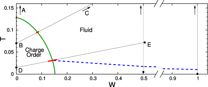
In this Letter, we investigate these predictions via extensive Monte Carlo (MC) simulations of the Coulomb glass lattice model with on-site disorder efros . In addition, we study in detail the transition from the fluid to the charge-ordered phase (COP). For $W=0$, there is good numerical evidence for an Ising-like transition moebius . For $W\neq 0$, mean-field theory predicts a stable COP for $d=3$ Pankov and Dobrosavljević (2005); malik . Beyond mean field there is some numerical evidence that the COP survives small positional disorder overlin ; surer and on-site disorder moebius_talk , but neither the phase diagram nor the critical properties have been investigated. Our results are as follows: (i) A COP exists below the (approximate) phase boundary in Fig. 1. (ii) The fluid-COP transition is consistent with the Random Field Ising model (RFIM) universality class, which shows that the interaction is effectively screened near the transition. (iii) No GP is found for $T$ well below the mean-field $T_{\text{g}}$ Pankov and Dobrosavljević (2005), in agreement with the results of Ref. surer but at lower $T$ and in a wider range for $W$. (iv) Due to the long-range interaction, the glass correlation length increases rapidly and possibly diverges as $T\to 0$. (v) For large $W$, the DOS scales as $g(\epsilon,T)=T^{\delta}f(|\epsilon|/T)$ near the gap, with a saturated exponent $\delta\simeq 2.00$. (vi) As $W$ decreases, scaling breaks down above the COP, and an effective power law $g_{L}(\epsilon,T=0)\propto|\epsilon|^{\delta}$ holds with $\delta\gtrsim 3$, in contrast with Ref.surer . A more extended account will appear later gp .

Model and simulation – We study the Hamiltonian

$$\mathcal{H}=\frac{e^{2}}{2\kappa}\sum_{i\neq j}(n_{i}-K)\frac{1}{|{\bf r}_{ij}|}(n_{j}-K)+W\sum_{i}n_{i}\varphi_{i}$$ (1)

where $n_{i}\in\{0,1\}$ are the occupation numbers for the $N=L^{d}$ sites of a hypercubic lattice ($d=3$) with $\sum_{i=1}^{N}n_{i}=KN$, and ${\bf r}_{ij}$ is the distance from $i$ to $j$. The filling factor is $K=1/2$ (which gives $\mu=0$). The random on-site energies $\varphi_{i}$ are independen and Gaussian-distributed with zero mean and variance unity. Energies and temperatures will be in units of $e^{2}/({\kappa}\ell)$ and lengths in units of the lattice spacing $\ell$.

We carry out canonical MC sampling along the paths ABC and ADE in Fig. 1 and at constant $W=0.2,0.5,1,2,4$. We consider an infinite sphere of periodic images of a central $L^{3}$ cell and sum over all interactions with the Ewald method with a dipole surface term leeuw . To reach low temperatures, we use the exchange MC algorithm exchange . For each realization (sample) $\varphi=\{\varphi_{i}\}_{i=1}^{N}$, we simulate identical replicas with different ($T,W$) along the simulation path. Every $N/2$ Metropolis steps for single-electron hops, replicas at adjacent $(T,W)$, $(T^{\prime},W^{\prime})$ swap their configurations with probability $\min(1,p)$, where $p=\exp[(\beta-\beta^{\prime})(\mathcal{H}-\mathcal{H}^{\prime})+(W^{\prime}-W)(\beta\mathcal{R}^{\prime}-\beta^{\prime}\mathcal{R})]$, $\beta=1/T$, and $\mathcal{R}=\sum_{i}n_{i}\varphi_{i}$, which preserves detailed balance. The simulation time $t_{s}$ is chosen so that averages over the intervals $[t_{s}/3,t_{s}]$ and $[t_{s}/9,t_{s}/3]$ agree within the statistical errors, and that the identity $2TN^{-1}[\langle\mathcal{R}\rangle]_{av}=W(2N^{-1}\sum_{i=1}^{N}[\langle n_{i}^{(a)}n_{i}^{(b)}\rangle]_{av}-1)$, valid for Gaussian disorder, is satisfied. Here, $\langle\cdot\rangle$ and $[\cdot]_{av}$ are the thermal and sample averages and $a,b$ are two independently simulated replicas with the same ($\varphi,T,W$) method .

Charge ordering – Fig.2 (top inset) shows the COP order parameter $M_{s}=[\langle|m_{s}|\rangle]_{av}$ along the paths AB, BC, and DE, where $m_{s}=N^{-1}\sum_{i=1}^{N}\sigma_{i}$ and $\sigma_{i}=S_{i}(-1)^{x_{i}+y_{i}+z_{i}}$ (we introduce the Ising variables $S_{i}=2n_{i}-1$). The sharp increase demonstrates a transition to a COP. To determine the transition temperature $T_{\text{c}}$, we measure the finite-size correlation length (CL) cooper

$$\xi_{\tiny{L}}=\frac{1}{2\sin(|{\bf k}_{\text{min}}|/2)}\left(\frac{\chi_{L}({\bf 0})}{\chi_{L}({\bf k}_{\text{min}})}-1\right)^{1/2}\,,$$ (2)

where $\chi_{L}({\bf k})=N^{-1}\sum_{i,j}[\langle\sigma_{i}\sigma_{j}\rangle]_{av}e^{i{\bf k}\cdot{\bf r}_{ij}}$ and ${\bf k}_{\text{min}}=(2\pi/L,0,0)$. Along BC, the data for $\xi^{{\mbox{{\tiny}}}}_{L}(T)/L$ for different $L$ cross (Fig.2, main panel), which signals ballesteros2 a transition at $T_{\text{c}}^{\text{BC}}=0.0950(15)$. We observe similar crossings along AB and DE (not shown) at $T_{\text{c}}^{\text{AB}}=0.1280(15)$, in excellent agreement with Refs.overlin ; moebius , and $T_{\text{c}}^{\text{DE}}=0.031(2)$. The curve $(T_{\text{c}}(W)/T_{\text{c}}^{\text{AB}})^{1.60}=1-(W/0.15)^{1.60}$ interpolates these three points and gives the approximate fluid-COP phase boundary in Fig. 1.

Figure 2: (Color online) Charge-order CL along path BC in Fig. 1. Top inset: order parameter $M_{s}$ along paths AB, BC, and DE. Bottom inset: specific heat along path BC.

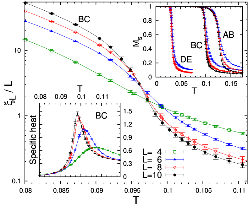
Critical behavior – Since at $W=0$ the fluid-COP transition has a positive specific-heat exponent moebius , disorder is relevant and the $W\neq 0$ transition will be governed by a random fixed point which, by analogy with the RFIM moebius , we expect to be at $T=0$ fisher . Assuming that the $W\neq 0$ transition is second order (indeed the distribution of $m_{s}$ is unimodal at all $T$ for a predominant, and increasing with $L$, fraction of the samples gp ) we obtain the critical exponents in Table I. $\beta/\nu$ and $\bar{\gamma}/\nu$ were estimated with the quotient method ballesteros for the observables $M_{s}$ and $\bar{\chi}^{{\mbox{{\tiny}}}}_{L}=N[\langle{m_{s}}^{2}\rangle]_{av}$ respectively [the quotient estimates from $(L,L^{\prime})=(6,8),(6,10)$ and $(8,10)$ agree within the errors], while $\gamma/\nu$ was obtained by fitting $aL^{\gamma/\nu}$ to the height of the peak of the susceptibility $N[\langle{m_{s}}^{2}\rangle-\langle|{m_{s}}|\rangle^{2}]_{av}$ (data not shown). The peak height for the specific heat $c_{L}=1/(NT^{2})[\langle\mathcal{H}^{2}\rangle-\langle\mathcal{H}\rangle^{2}]_{av}$ increases slowly with $L$ (Fig. 2, bottom inset), which suggests either $\alpha<0$ or a logarithmic divergence ($\alpha=0$). We could not directly estimate $\nu$ in a reliable way, but we obtain $\nu=1.11(12)$ from the modified hyperscaling relation fisher $(d-\theta)\nu=2-\alpha$, assuming $\alpha=0$ and using $\theta=\bar{\gamma}/\nu-\gamma/\nu=1.20(20)$. As shown in Table I, the exponents agree fairly well with the known values for the RFIM middleton , which suggests that the interaction is effectively short-range near the phase boundary.

Table 1: Critical exponents for the fluid-COP transition along BC in Fig. 1, compared with the RFIM values middleton .

	$\gamma/\nu\hphantom{2}$	$\bar{\gamma}/\nu\hphantom{2}$	$\beta/\nu\hphantom{2}$	$\nu\hphantom{2}$
Coulomb glass	$1.69(17)$	$2.89(9)$	$0.06(4)$	$1.11(12)$
RFIM	$1.44(12)$	$2.93(11)$	$0.011(4)$	$1.37(9)$

Glass phase – Several works have searched for a GP by measuring the parameter $[(\langle n_{i}\rangle-1/2)^{2}]_{av}$ davies or higher cumulants of the overlap between two replicas diaz . We measure instead the glass CL $\xi^{{\mbox{{\tiny G}}}}_{\tiny{L}}$ obtained from Eq. (2) by replacing $[\langle\sigma_{i}\sigma_{j}\rangle]_{av}$ with the “spin-glass” correlation function $G({\bf r}_{ij})=[(\langle S_{i}S_{j}\rangle-\langle S_{i}\rangle\langle S_{j}\rangle)^{2}]_{av}$. In the fluid phase we have $G(r)\sim\exp(-r/\xi^{{\mbox{{\tiny G}}}})$ for $\xi^{{\mbox{{\tiny G}}}}<r\ll L$, where $\xi^{{\mbox{{\tiny G}}}}$ is the bulk CL, thus $\xi^{{\mbox{{\tiny G}}}}_{L}\sim\xi^{{\mbox{{\tiny G}}}}$ for $L\gg\xi^{{\mbox{{\tiny G}}}}$ and $\xi^{{\mbox{{\tiny G}}}}_{L}\sim L$ for $L\ll\xi^{{\mbox{{\tiny G}}}}$. In a “many-state” GP mueller , $G(r)$ tends to a constant for large $r$, thus we have $\xi^{{\mbox{{\tiny G}}}}_{L}\sim L^{d/2+1}$. Hence the existence of a GP will be signaled by the crossing of $\xi^{{\mbox{{\tiny G}}}}_{L}(T)/L$ for different $L$ near $T=T_{\text{g}}$ ballesteros2 .

Figure 3: (Color online) (a) Glass correlation length $\xi^{{\mbox{{\tiny G}}}}_{L}$ at $W=1$ and $W=0.5$ (shifted upwards by a factor 7). The absence of crossing is evidence against the existence of an equilibrium glass transition. (b) Power-law fit of $\xi_{10}^{{\mbox{{\tiny G}}}}=cT^{-\nu^{\prime}}$ for $W=1$. (c) Scaling plot $\xi^{{\mbox{{\tiny G}}}}_{L}=Lf(TL^{1/\nu^{\prime}})$ for $W=1$ and $W=0.5$ (shifted to the right by a factor 5).

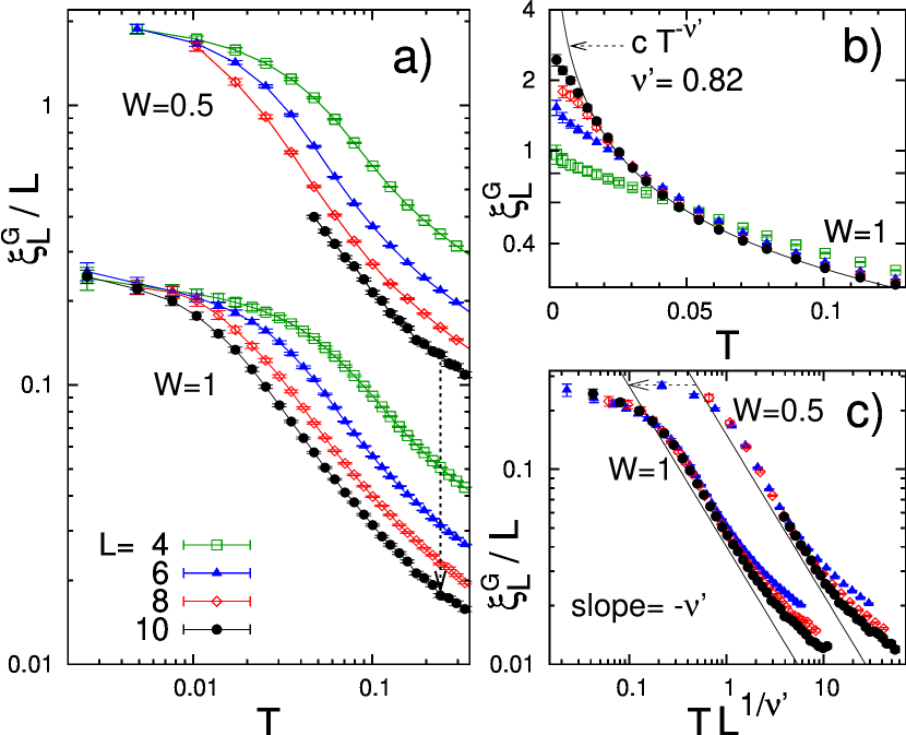
As shown in Fig.3(a) for $W=0.5,1$, we observe no crossing down to the lowest equilibrated temperature and well below the mean-field glass transition ($T_{\text{g}}\approx 0.037$ for $W=0.5$ Pankov and Dobrosavljević (2005)). Similar results were found in Ref.surer for $T\geq 0.03$ and $W\leq 0.4$. We also exclude that a GP occurs at $T_{\text{g}}>T_{\text{c}}$ along BC and DE by comparing the crossing temperatures for $\xi^{{\mbox{{\tiny G}}}}_{L}/L$ (not shown) and $\xi^{{\mbox{{\tiny}}}}_{L}/L$: For all pairs $(L,L^{\prime})$ they differ by less than $1\%$. Together with the results at constant $W$, this indicates that no GP exists above the dashed line in Fig. 1.

Fig. 3(b) shows that $\xi^{{\mbox{{\tiny G}}}}_{L}$ is nearly independent of $L$ at large $T$ and $W=1$ apart from small finite-size effects, thus $\xi^{{\mbox{{\tiny G}}}}_{L=10}$ is a good estimate of $\xi^{{\mbox{{\tiny G}}}}$ for $T\gtrsim 0.017$. At lower $T$ we observe $\xi^{{\mbox{{\tiny G}}}}_{L}\sim L$, which shows that $\xi^{{\mbox{{\tiny G}}}}$ becomes larger than $\simeq 10$, and possibly diverges as $T\to 0$. Indeed, $\xi_{L=10}^{{\mbox{{\tiny G}}}}(T)$ can be fitted for $T\in[0.017,0.113]$ by a power law $T^{-\nu^{\prime}}$ with $\nu^{\prime}=0.82$ [Fig. 3(b)], which also gives a satisfactory finite-size scaling $\xi^{{\mbox{{\tiny G}}}}_{L}=Lf(TL^{1/\nu^{\prime}})$ [Fig. 3(c)]. A divergence would be a nontrivial prediction, since for $W\neq 0$ the ground state of a periodic sample is unique. Because $L$ and $\xi^{{\mbox{{\tiny G}}}}_{L}$ are rather small, however, we cannot rule out neither that $\xi^{{\mbox{{\tiny G}}}}$ stays finite at $T=0$, nor an exponent $\nu^{\prime}=1$. An interesting question is whether there is a link with the $T^{-1}$ divergence of the screening length found in mean-field theory mueller and from simple arguments hunt ; tf . We tested that the CL obtained by replacing $[\langle\sigma_{i}\sigma_{j}\rangle]_{av}$ with $[\langle\sigma_{i}\sigma_{j}\rangle-\langle\sigma_{i}\rangle\langle\sigma_{j}\rangle]_{av}$ in Eq. (2), remains smaller than unity at all $T$, which suggests that the correlated regions are disordered. Finally, we simulated the short-range RFIM choosing $W$ so that the value of $N^{-1}[\langle\sum_{i}n_{i}\varphi_{i}\rangle]_{av}$ is close to the Coulomb glass value at $W=1$, and found $\xi^{{\mbox{{\tiny G}}}}_{L}\leq 1$ as $T\to 0$, which suggests that the large CL is due to the long-range interaction.

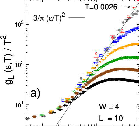
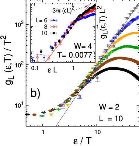
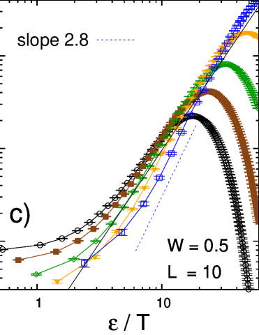
Coulomb gap – The single-particle DOS is defined as $g_{L}(\epsilon,T)=N^{-1}[\langle\sum_{i=1}^{N}\delta(\epsilon-\epsilon_{i})\rangle]_{av}$ where $\epsilon_{i}=\sum_{j\neq i}(n_{j}-K)/r_{ij}+W\varphi_{i}$ is the cost of adding an electron at site $i$ of the central cell while leaving the periodic images unchanged. We compute the infinite sum with the Ewald method. Because of the dipole term leeuw , the DOS has no hard gap dipole ; gp , unlike for a finite, nonperiodic system. The finite-size effects due to the energy scale $L^{-1}$ turn out to be significant for $|\epsilon|\leq aL^{-1}$ with $a\simeq 0.3$, while those due to the sample fluctuations of $\mu$ (of order $W/L^{d/2}$) were drastically reduced by shifting the DOS before averaging over the samples shift . In the gap region $(|\epsilon|,T)\ll\Delta$, which is our only focus here, one expects the scaling $g_{L}(\epsilon,T)=T^{\delta}f(|\epsilon|/T)$ for $aL^{-1}\ll(|\epsilon|,T)$, with $f(x)\sim$ constant as $x\to 0$ and $f(x)\sim c\,x^{\delta}$ as $x\to\infty$. Fig. 4(a,b,c) show scaling plots with $\delta=2$ for $L=10$ and $W=4,2,0.5$. For $W=4$ scaling is excellent even for this moderate size, with small deviations for $|\epsilon|\lesssim 0.03$ due to finite-size effects. For $\Delta/T\gg|\epsilon|/T\gtrsim 6$ the data are well fitted by $g_{10}(\epsilon,T)=c|\epsilon|^{2}$ with $c\simeq 1.1$, which is close to the self-consistent prediction $c=3/\pi$ efros (while Ref.mueller finds $c=0.2083$). As shown in Fig. 4(b) (inset), the finite-size scaling ansatz $g_{L}(\epsilon,T)=L^{-\delta}h(\epsilon L)$, which should hold for $T\ll|\epsilon|\ll aL^{-1}\ll\Delta$ [with $h(x)\sim c|x|^{\delta}$ for large $x$], is also well satisfied with $c=3/\pi$, $\delta=2$. Our final estimate is $\delta=2.01\pm 0.05$, which provides strong support for a saturated ES bound.

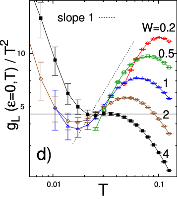
For decreasing $W$, we observe increasingly stronger deviations from the $\delta=2$ scaling. A fit $g_{10}(\epsilon,T)=c|\epsilon|^{\delta}$ at low $T$ gives an effective exponent $\delta\simeq 2.3$ for $W=2$ and $\delta\geq 2.8$ for $W=0.5$ [Fig. 4(c)]. We interpret this as a crossover due to the vicinity of the fluid-COP boundary, below which the DOS has a hard gap at $T=0$. The crossover is apparent in Fig. 4(d): Since $g_{L}(\epsilon=0,T)/T^{2}\propto T^{\delta-2}$ for $aL^{-1}\leq T\leq\Delta$, the plateau for $W=4$ supports $\delta=2$, while for decreasing $W$ the exponent increases to $\delta>3$. The $L$ dependence is consistent with the scaling $g_{L}(\epsilon=0,T)=T^{\delta}h(TL)$ (not shown) with $\delta$ extracted from Fig.4(d) for each value of $W$. Our results differ markedly from Ref.surer , which reports $\delta=1.83(3)$ for the same model at $W=0.4$, $T=0$ [however, $g_{L}(\epsilon\simeq 0)$ is much larger than our data, and increases with $L$]. A similar crossover in the DOS was reported for $d=2$, where the COP occurs at $W=0$ pikus .

Figure 4: (Color online) (a,b,c) Scaling plots of the DOS for $W=4,2,0.5$ and $L=10$. From bottom to top: $T=0.047,0.035,0.025,0.017,0.0105$ plus $T=0.0049$ for $W=4,2$ and $T=0.0026$ for $W=4$. The error is the standard deviation of the sample fluctuations. The solid lines represent the ES law $g(\epsilon,T)=3\,\epsilon^{2}/\pi$. The dashed line with slope 2.8 in (c) highlights the departure from the ES law at low $W$ (the $W=0.5,T=0.0105$ data are not fully equilibrated, but the slope increases with simulation time). Inset of (b) Finite-size scaling for $W=4$ and $T=0.0077$ (other values of $W$ and $T$ give similar plots). (d) Temperature dependence of the DOS at $|\epsilon|\leq 0.0075$ for $L=10$.

In conclusion, we presented evidence that no equilibrium glass phase exists in the Coulomb glass, but a saturated ES bound holds. The long-range part of the interaction appears to be irrelevant as to the equilibrium thermodynamics, except for a possible diverging correlation length at $T=0$, which calls for further investigation.

We thank M. Müller, V. Dobrosavljevic, A.L. Efros, H. Katzgraber, A. Möbius, and G. Zimanyi for discussions. This work is supported by the Generalitat de Catalunya and the Ministerio de Ciencia e Innovación (FIS-2006-13321-C02-01, AP2007-01005). The computations were performed on the BSC-RES node at Universidad de Cantabria and the Albeniz cluster at UB. MP thanks the Aspen Center for Physics for hospitality.

References

- (1) A. L. Efros and B. I. Shklovskii, J. Phys. C 8, L49 (1975).
- (2) See e.g. A. Möbius, J. Phys. C 18, 4639 (1985); A.G. Zabrodskii, Phil. Mag. B 81, 1131 (2001).
- (3) Q. Li and P. Phillips, Phys. Rev. B 49, 10269 (1994).
- Möbius et al. (1992) A. Möbius, M. Richter, and B. Drittler, Phys. Rev. B 45, 11568 (1992).
- (5) M. Sarvestani, M. Schreiber, and T. Vojta, Phys. Rev. B 52, R3820 (1995).
- (6) M.H. Overlin, L.A. Wong, and C. C. Yu, Phys. Rev. B 70, 214203 (2004).
- (7) B. Surer, H. G. Katzgraber, G. T. Zimanyi, B. A. Allgood, and G. Blatter, Phys. Rev. Lett. 102, 067205(2009).
- (8) E. I. Levin, V. L. Nguyen, B. I. Shklovskii, and A. L. Efros, Sov. Phys. JETP 66, 842 (1987).
- (9) T. Vojta, W. John, and M. Schreiber, J. Phys. Condens. Matter 5, 4989 (1993).
- (10) A. Hunt, Philos. Mag. Lett. 62, 371 (1990).
- (11) J. H. Davies, P. A. Lee, and T. M. Rice, Phys. Rev. B 29, 4260 (1984).
- (12) See e.g. Ref.mueller and references therein.
- (13) M. Müller and S. Pankov, Phys. Rev. B 75, 144201 (2007).
- (14) E. R. Grannan and C. C. Yu, Phys. Rev. Lett. 71, 3335 (1993).
- (15) A. Díaz-Sánchez, M. Ortuño, A. Pérez-Garrido, and E. Cuevas, Phys. Stat. Sol. (b) 218, 11 (2000).
- (16) J.R.L. de Almeida and D.J. Thouless, J. Phys. A 11, 983 (1978).
- (17) A. A. Pastor and V. Dobrosavljević, Phys. Rev. Lett. 83, 4642 (1999).
- Pankov and Dobrosavljević (2005) S. Pankov and V. Dobrosavljević, Phys. Rev. Lett. 94, 046402 (2005).
- Müller and Ioffe (2004) M. Müller and L. B. Ioffe, Phys. Rev. Lett. 93, 256403 (2004).
- (20) A. L. Efros, J. Phys. C 9, 2021 (1976).
- (21) A. Möbius and U. K. Rößler, arxiv:0904.3723 (2009).
- (22) V. Malik and D. Kumar, Phys. Rev. B 76, 125207 (2007).
- (23) A. Möbius, talk given at TIDS11 (2005).
- (24) M. Goethe and M. Palassini, in preparation.
- (25) S. W. de Leeuw, J. W. Perram, E. R. Smith, Proc. R. Soc. London, Ser. A 373, 27 (1980).
- (26) K. Hukushima and K. Nemoto, J. Phys. Soc. Japan 65, 1604 (1996).
- (27) The largest size simulated is and the number of pairs is , for (ABC, ADE, constant), respectively. The number of samples is between 100 and 676 for , depending on the path, and larger for . For each triplet , we simulate four independent replicas to obtain an unbiased estimate of . We used MC sweeps per replica for paths ABC and , and for ADE, for a total of about computing hours.
- (28) F. Cooper, B. Freedman, and D. Preston, Nucl. Phys. B 210, 210 (1982).
- (29) H. G. Ballesteros et al., Phys. Rev. B 62, 14237 (2000); M. Palassini and S. Caracciolo, Phys. Rev. Lett. 82, 5128 (1999).
- (30) See e.g. D. S. Fisher, Phys. Rev. Lett. 56, 416 (1986).
- (31) H. G. Ballesteros, L. A. Fernández, V. Martín-Mayor, and A. Muñoz Sudupe, Phys. Lett. B 378, 207 (1996).
- (32) A. A. Middleton and D. S. Fisher, Phys. Rev. B 65, 134411 (2002).
- (33) A naive application of the Thomas-Fermi theory gives a screening length diverging as .
- (34) The energy change for an electron hop from to in all images receives a positive contribution .
- (35) For each sample we shift by , where .
- (36) F.G. Pikus and A.L. Efros, Phys. Rev. Lett. 73, 3014 (1994).