Multiparameter entangled state engineering using adaptive optics

Abstract

We investigate how quantum coincidence interferometry is affected by a controllable manipulation of transverse wave-vectors in type-II parametric down conversion using adaptive optics techniques. In particular, we discuss the possibility of spatial walk-off compensation in quantum interferometry and a new effect of even-order spatial aberration cancellation.

I Introduction

Quantum entanglement Schroedinger (1935) is a valuable resource in many areas of quantum optics and quantum information processing. One of the most widespread techniques for generating entangled optical states is spontaneous parametric downconversion (SPDC) Klyshko (1967); Harris et al. (1967); Giallorenzi and Tang (1968); Kleinmann (1968). SPDC is a second-order nonlinear optical process in which a pump photon is split into a pair of new photons with conservation of energy and momentum. The phase-matching relation establishes conditions to have efficient energy conversion between the pump and the downconverted waves, called signal and idler. This condition sets also a specific relation between the frequency and the emission angle of down converted radiation. In other words, the quantum state emitted in the SPDC process cannot be factorized into separate frequency and wavevector components. This leads to several interesting effects where the manipulation of a spatial variable affects the shape of the polarization-temporal interference pattern. For example, the dependence of polarization-temporal interference on the selection of collected wavevectors was studied in detail in Atature et al. (2002).

Here we engineer the quantum state in the space of transverse momentum and we study how this spatial modulation is transferred to the polarization-spectral domain by means of quantum interferometry. We will focus on type-II SPDC using birefringent phase-matching since the correlations between wave-vectors and spectrum are stronger than employing other phase-matching conditions.

Our aim is twofold. From one point of view, we study the effect of spatial modulations on temporal quantum interference. This could be useful, for example, in quantum optical coherence tomography (QOCT) Abouraddy et al. (2002); Nasr et al. (2003). When focusing light on a sample with non-planar surface, the photons will acquire a spatial phase distribution in the far-field, which may perturb the shape of the interference dip. Our results will provide a tool to understand this effect.

From a second point of view, we would like to study and characterize spatial modulation as a tool for quantum state engineering. This may find application in the field of quantum information processing, where it is important to gain a high degree of control over the production of quantum entangled states entangled in one or more degrees of freedom (hyper-entanglement).

We start (Section II) introducing a theoretical model of a type-II quantum interferometer, comprising the polarization, spectral and spatial degrees of freedom. A modulation in the wave-vector space is provided by an adaptive optical setup and equations for the polarization-temporal interference pattern in the coincidence rate are derived. In our analysis (Section III) we will highlight and discuss theoretically two interesting special cases. The first one is the possibility of restoring high visibility in type-II quantum interference with large collection apertures. In some situations, to collect a higher photon flux or a broader photon bandwidth, it can be useful to enlarge the collection apertures of the optical system. But, when dealing with type-II SPDC in birefringent crystals, for large collection apertures the effect of spatial walkoff introduces distinguishability between the photons, leading to a reduced visibility of temporal and polarization quantum interference. We will show that high visibility can be restored with a linear phase shift along the vertical axis.

The second effect is the spatial counterpart of spectral dispersion cancellation Franson (1995); Steinberg et al. (1992). In the limit of large detection apertures, the correlations between the photons momenta will cancel out the effects of even-order aberrations, exactly as in the limit of slow detectors the frequency correlations cancel out the even-order terms of spectral dispersion. The experimental demonstration of this effect has been reported recently Bonato et al. (2008).

Finally, in Section IV, we introduce a numerical approach for practical evaluation of the results of the theoretical model, discussing a few examples. By means of this approximated model, we will examine under what conditions the even-order aberration cancellation effect can be observed (Section V).

II Theoretical model

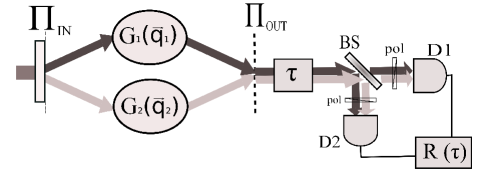
Figure 1: Scheme of the proposed setup. Horizontally-polarized photons from type-II SPDC are assigned a phase dependent on the photon transverse momentum $\phi_{o}(q_{o})$, while the vertically-polarized ones are assigned a phase $\phi_{e}(q_{e})$. The modulated photons enter a type-II quantum interferometer, which records the coincidence count rate as a function of the delay $\tau$ between the photons given by an appropriate delay-line.

Consider the scheme in Fig. 1. A laser beam pumps a $\chi^{(2)}$ nonlinear material phase-matched for type-II parametric down-conversion, creating a pair of entangled photons. Each of the generated photons passes through a Fourier transform system, then enters a modulation system which transforms each transverse wave-vector for the horizontally polarized photon according to the transfer function $G_{1}(\mathbf{q_{1}})$ and for the vertically-polarized photon according to $G_{2}(\mathbf{q_{2}})$. After being modulated in the $q$-space, the photons enter a type-II interferometer. A non-polarizing beamsplitter creates polarization entanglement from the polarization-correlated pair emitted by the source. The beams at the output ports of the beamsplitter are directed towards two single photon detectors. Two polarizers at 45 degrees before the BS restore indistinguishability in the polarization degree of freedom. An adjustable delay-line $\tau$ is scanned and the coincidence rate $R(\tau)$ between the detection events of the two detectors is recorded. An aperture is placed before the beamsplitter to select an appropriate collection angle.

II.1 Notation

Consider a monochromatic plane wave of complex amplitude $E(\mathbf{r})=E_{0}e^{-i\mathbf{k}\cdot\mathbf{r}}$ with $\mathbf{r}=(x,y,z)$. For a given wavelength $\lambda$, corresponding to a frequency $\Omega$, the wave-vector can be split in a transverse component $\mathbf{q}=(q_{x},q_{y})$ and a longitudinal component $\beta(\mathbf{q};\Omega)$:

$$\mathbf{k}=[\mathbf{q},\beta(\mathbf{q};\Omega)]$$ (1)

The wave-number is:

$$k(\Omega)=\frac{n(\Omega)\Omega}{c}$$ (2)

The longitudinal component of the wave-vector is:

$$\beta(\mathbf{q},\Omega)=\sqrt{k^{2}(\Omega)-|\mathbf{q}|^{2}}$$ (3)

Therefore the electric field at the position $\mathbf{r}$ and time $t$ can be written as:

$$E(\mathbf{r};t)=\int d\mathbf{q}\int d\Omega\tilde{E}(\mathbf{q},\Omega)e^{-i\mathbf{q}\cdot\mathbf{\rho}}e^{-i\beta(\mathbf{q};\Omega)z}e^{i\Omega t}$$ (4)

where $\mathbf{\rho}=(x,y)$.

In paraxial approximation $|\mathbf{q}|^{2}\ll k^{2}(\Omega)$, so that:

$$\beta(\mathbf{q},\Omega)\approx k(\Omega)-\frac{|\mathbf{q}|^{2}}{2k(\Omega)}$$ (5)

For a quasi-monochromatic wave-packet centered around the frequency $\Omega_{0}$ one can write $\Omega=\Omega_{0}+\nu$, with $\nu\ll\Omega_{0}$ and this expression can be approximated by:

$$\beta(\mathbf{q},\Omega)\approx k_{0}+\frac{\nu}{u_{0}}-\frac{|\mathbf{q}|^{2}}{2k_{0}}$$ (6)

where $k_{0}=k(\Omega_{0})$ and $u_{0}=\left(\frac{dk(\Omega)}{d\Omega}|_{\Omega=\Omega_{0}}\right)^{-1}$ is the group velocity for the propagation of the wave-packet through the material.

II.2 State Generation

Using first-order time-dependent perturbation theory the two-photon state at the output of the nonlinear cystal can be calculated as:

$$\left|\psi\right\rangle\sim-\frac{i}{\hbar}\int dtH_{I}(t)\left|0\right\rangle$$ (7)

where the interaction Hamiltonian is:

$$H_{I}(t)=\frac{1}{V}\int d\mathbf{r}\chi^{(2)}(\mathbf{r})E_{p}^{(+)}(\mathbf{r},t)E_{s}^{(-)}(\mathbf{r},t)E_{i}^{(-)}(\mathbf{r},t)$$ (8)

The strong, undepleted pump beam can be treated classically. Assuming a monochromatic plane-wave propagating along the z direction:

$$E_{p}(\mathbf{r},t)=E_{p}e^{i(k_{p}z-\omega_{p}t)}$$ (9)

The signal and idler photons are described by the following quantum field operators:

$$\hat{E}_{i}^{(-)}(\mathbf{r},t)=\int d\mathbf{q}_{i}\int d\omega_{i}e^{i[\beta(\mathbf{q}_{i},\omega_{i})z+\mathbf{q}_{i}\cdot\mathbf{\rho}-\omega_{i}t]}\hat{a}(\mathbf{q}_{i},\omega_{i})$$ (10)

The biphoton quantum state at the output plane of the nonlinear crystal is Rubin (1996):

$$\left|\psi\right\rangle=\int d\mathbf{q}\int d\nu\tilde{\Phi}(\mathbf{q},\nu)\hat{a}_{o}^{\dagger}(\mathbf{q},\Omega_{0}+\nu)\hat{a}_{e}^{\dagger}(\mathbf{-q},\Omega_{0}-\nu)\left|0\right\rangle$$ (11)

Two photons are emitted from the nonlinear crystal, one horizontally-polarized (ordinary photon) and the other vertically-polarized (extraordinary photon), with anticorrelated frequencies and emission directions.

In the case of a single bulk crystal of thickness L and constant nonlinearity $\chi_{o}$, the probability amplitude for having the signal photon in the mode $(\mathbf{q},\Omega_{0}+\nu)$ and the idler in the mode $(-\mathbf{q},\Omega_{0}-\nu)$:

$$\tilde{\Phi}(\mathbf{q},\nu)=\mbox{sinc}\left[\frac{L\Delta(\mathbf{q},\nu)}{2}\right]e^{i\frac{\Delta(\mathbf{q},\nu)L}{2}}$$ (12)

For type-II collinear degenerate phase-matching, the phase-mismatch function $\Delta(\mathbf{q},\nu)$ can be approximated to be:

$$\Delta(\mathbf{q},\nu)=-\nu D+M\mathbf{\hat{e}_{2}}\cdot\mathbf{q}+\frac{2|\mathbf{q}|^{2}}{k_{p}}$$ (13)

where D is the difference between the inverse of the group velocities of the ordinary and extraordinary photons inside the birefringent crystal and the quadratic term in $\mathbf{q}$ is due to diffraction in paraxial approximation. The last term is the first-order approximation for the spatial walk-off.

II.3 Propagation

Consider a photon described by the operator $\hat{a}_{j}(\mathbf{q},\Omega)$ (polarization $j=e,o$, frequency $\Omega$, and transverse momentum $\mathbf{q}$). Its propagation through an optical system to a point $\mathbf{x}_{k}$ on the output plane is described by the optical transfer function $H_{j}(\mathbf{x}_{k},\mathbf{q};\Omega)$. In our setup, the field at the detector will be a superposition of contributions from the ordinary and extraordinary photons. The quantized electric fields at the detector planes are:

$$\begin{split}\hat{E}_{A}^{(+)}(\mathbf{x}_{A},t_{A})&=\int d\mathbf{q}\int d\omega e^{i\omega t_{A}}[H_{e}(\mathbf{x_{A}},\mathbf{q};\omega)\hat{a}_{e}(\mathbf{q},\omega)\\ &\qquad+H_{o}(\mathbf{x_{A}},\mathbf{q};\omega)\hat{a}_{o}(\mathbf{q},\omega)]\\ \hat{E}_{B}^{(+)}(\mathbf{x}_{B},t_{B})&=\int d\mathbf{q}\int d\omega e^{i\omega t_{B}}[H_{e}(\mathbf{x_{B}},\mathbf{q};\omega)\hat{a}_{e}(\mathbf{q},\omega)+\\ &\qquad H_{o}(\mathbf{x_{B}},\mathbf{q};\omega)\hat{a}_{o}(\mathbf{q},\omega)]\end{split}$$ (14)

The probability amplitude to detect a photon pair at the detector planes, with space-time coordinates $(\mathbf{x_{A}},t_{A})$ and $(\mathbf{x_{B}},t_{B})$, is:

$$A(\mathbf{x_{A}},\mathbf{x_{B}};t_{A},t_{B})=\left\langle 0\right|\hat{E}_{A}^{(+)}(\mathbf{x}_{A},t_{A})\hat{E}_{B}^{(+)}(\mathbf{x}_{B},t_{B})\left|\psi\right\rangle$$ (15)

For the biphoton probability amplitude we get:

$$\begin{split}&A(\mathbf{x_{A}},\mathbf{x_{B}};t_{A},t_{B})=\int d\mathbf{q_{o}}d\mathbf{q_{e}}d\omega_{o}d\omega_{e}\Phi(\mathbf{q_{o}},\mathbf{q_{e}};\omega_{o},\omega_{e})\\ &\qquad\Bigl{[}H_{e}(\mathbf{x_{A}},\mathbf{q_{e}};\omega_{e})H_{o}(\mathbf{x_{B}},\mathbf{q_{o}};\omega_{o})e^{-i(\omega_{e}t_{A}+\omega_{o}t_{B})}+\\ &\qquad H_{o}(\mathbf{x_{A}},\mathbf{q_{o}};\omega_{o})H_{e}(\mathbf{x_{B}},\mathbf{q_{e}};\omega_{e})e^{-i(\omega_{o}t_{A}+\omega_{e}t_{B})}\Bigr{]}\end{split}$$ (16)

This probability amplitude represents the superposition of two possible events leading to a coincidence count in the detectors:

1. the V-polarized photon with momentum $\mathbf{q_{e}}$ and frequency $\omega_{e}$ going through the lower branch to arrive at position $x_{A}$ in detector A, while the H-polarized photon with momentum $\mathbf{q_{o}}$ and frequency $\omega_{o}$ goes through the upper branch to arrive at position $x_{B}$ in detector B.

2. the V-polarized photon with momentum $\mathbf{q_{e}}$ and frequency $\omega_{e}$ going through the lower branch to arrive at position $x_{B}$ in detector B, while the H-polarized photon with momentum $\mathbf{q_{o}}$ and frequency $\omega_{o}$ goes through the upper branch to arrive at position $x_{A}$ in detector A.

Since the superposition is coherent, there are quantum interference effects between the two probabilities amplitudes.

II.3.1 State engineering section

In the state engineering section, each of the two branches consists of a pair of achromatic Fourier-transform systems coupled by a spatial light modulator or a deformable mirror. Each Fourier-transform system consists of a single lens of focal length $f$, separated from the optical elements before and after it by a distance $f$. The first Fourier system maps each incident transverse wave-vector $\mathbf{q}$ on the plane $\Pi_{IN}$ to a point $\mathbf{x}(\mathbf{q})$ on the Fourier plane $\Pi_{F}$:

$$\mathbf{x}(\mathbf{q})=\frac{f}{k_{0}}\mathbf{q}\qquad k_{0}=\frac{\Omega_{0}}{c}$$ (17)

where f is the focal length of the Fourier-transform system. Since we assume the system is achromatic for a certain bandwidth around a central frequency $\Omega_{0}$, the position $\mathbf{x}(\mathbf{q})$ depends only on $\mathbf{q}$ and not on $\omega$.

The spatial modulator assigns a different amplitude and phase to the light incident on each point, as described by the function $G(\mathbf{x})=t(\mathbf{x})e^{i\varphi(\mathbf{x})}$. Each point is then mapped back to a wave-vector on the plane $\Pi_{OUT}$ by the second achromatic Fourier-transform system.

Using the formalism of Fourier optics Goodman (1996), the transfer function between the planes $\Pi_{IN}$ and $\Pi_{OUT}$ can be calculated to be:

$$h_{1}(\mathbf{x_{1}},\mathbf{x_{3}})=\int d\mathbf{x}\quad G(\mathbf{x})\quad e^{-i\frac{k_{0}}{f}\mathbf{x}\cdot(\mathbf{x_{1}}+\mathbf{x_{3}})}$$ (18)

The corresponding momentum transfer function is:

$$H_{1}(\mathbf{q_{1}},\mathbf{q_{3}})=G\left[\frac{f}{k_{0}}\mathbf{q_{1}}\right]\delta(\mathbf{q_{1}}-\mathbf{q_{3}})$$ (19)

II.3.2 Interferometer

After the plane $\Pi_{OUT}$ the two photons enter a type-II quantum interferometer. Each propagates in free space to a birefringent delay-line and a detection aperture $p(\mathbf{x})$ to be finally focused to the detection planes by means of lenses of focal length $f_{0}$. Following the derivation in Atature et al. (2002) the transfer function is:

$$H_{2}(\mathbf{x_{i}},\mathbf{q};\omega) = \int h(\mathbf{x_{1}},\mathbf{x_{i}};\omega)e^{i\mathbf{q}\cdot\mathbf{x_{1}}}d\mathbf{x_{1}}$$ (20)

$$= e^{i(\omega/c)(d_{1}+d_{2}+f_{0})}\mbox{exp}\left[-i\frac{\omega|\mathbf{x_{i}}|^{2}}{2cf_{0}}\left(\frac{d_{2}}{f_{0}}-1\right)\right]$$

$$\qquad\cdot\;e^{-i(cd_{1}/2\omega)|\mathbf{q}|^{2}}\tilde{P}\left(\frac{\omega}{cf_{0}}\mathbf{x_{i}}-\mathbf{q}\right)$$

where $\tilde{P}(\mathbf{q})$ is the Fourier transform of $|p(\mathbf{x})|^{2}$.

A combination of the two different stages is described by the transfer function:

$$H_{\alpha}(\mathbf{x_{j}},\mathbf{q_{\alpha}};\omega_{\alpha})=G_{\alpha}\left[\frac{f}{k_{0}}\mathbf{q_{\alpha}}\right]H_{2}(\mathbf{x_{j}},\mathbf{q_{\alpha}};\omega),$$ (21)

where the two functions $G_{1}(\mathbf{q})$ and $G_{2}(\mathbf{q})$ are the momentum transfer function which describe the modulation imparted respectively on the ordinary and the extraordinary photon.

II.4 Detection

Since the single-photon detectors used in quantum optics experiments are slow with respect to the temporal coherence of the photons and their area is larger than the spot into which the photons are focused by the collection lens, we integrate over the spatial and temporal coordinates. Therefore the coincidence count-rate expressed in terms of the biphoton probability amplitude is:

$$R(\tau)=\int d\mathbf{x_{A}}\int d\mathbf{x_{B}}\int dt_{A}\int dt_{B}|A(\mathbf{x_{A}},\mathbf{x_{B}};t_{A},t_{B})|^{2}$$ (22)

Following the derivation described in Appendix A, one gets:

$$R(\tau)=R_{0}-\Lambda\left(1-\frac{2\tau}{DL}\right)W_{G}(\tau)$$ (23)

where $\Lambda(x)$ is the triangular function:

$$\Lambda(x)=\bigg{\{}\begin{array}[]{l}1-|x|,\qquad|x|\leq 1\\ 0,\qquad\qquad|x|>1\end{array}$$ (24)

Therefore, the coincidence count rate $R(\tau)$ is given by the summation of a background level $R_{0}$ and an interference pattern given by the triangular dip, $\Lambda\left(1-\frac{2\tau}{DL}\right)$, that one gets when working with narrow apertures, modulated by the function $W_{M}(\tau)$ which depends on the details of the adaptive optical system.

The expressions for $R_{0}$ and $W_{M}(\tau)$ are:

$$\begin{split}R_{0}&=\int d\mathbf{q}\int d\mathbf{q^{\prime}}\mbox{sinc}[ML\mathbf{\hat{e}_{2}}\cdot(\mathbf{q}-\mathbf{q^{\prime}})]G_{1}^{*}\left(\frac{f}{k_{0}}\mathbf{q}\right)G_{1}\left(\frac{f}{k_{0}}\mathbf{q^{\prime}}\right)G_{2}^{*}\left(-\frac{f}{k_{0}}\mathbf{q}\right)G_{2}\left(-\frac{f}{k_{0}}\mathbf{q^{\prime}}\right)\\ &\qquad\qquad\qquad\qquad e^{-i\frac{ML}{2}\mathbf{\hat{e}_{2}}\cdot(\mathbf{q}-\mathbf{q^{\prime}})}\quad e^{i\frac{2d_{1}}{k_{p}}[|\mathbf{q}|^{2}-|\mathbf{q^{\prime}}|^{2}]}\tilde{P}_{A}(\mathbf{q}-\mathbf{q^{\prime}})\tilde{P}_{B}(-\mathbf{q}+\mathbf{q^{\prime}})\end{split}$$ (25)

and

$$\begin{split}W_{M}(\tau)&=\int d\mathbf{q}\int d\mathbf{q^{\prime}}\mbox{sinc}\left[ML\mathbf{\hat{e}_{2}}\cdot(\mathbf{q}+\mathbf{q^{\prime}})\Lambda\left(1-\frac{2\tau}{DL}\right)\right]G_{1}^{*}\left(\frac{f}{k_{0}}\mathbf{q}\right)G_{1}\left(\frac{f}{k_{0}}\mathbf{q^{\prime}}\right)\\ &\qquad\qquad\qquad G_{2}^{*}\left(-\frac{f}{k_{0}}\mathbf{q}\right)G_{2}\left(-\frac{f}{k_{0}}\mathbf{q^{\prime}}\right)e^{-i\frac{M}{D}\tau\mathbf{\hat{e}_{2}}\cdot(\mathbf{q}-\mathbf{q^{\prime}})}e^{i\frac{2d_{1}}{k_{p}}[|\mathbf{q}|^{2}-|\mathbf{q^{\prime}}|^{2}]}\tilde{P}_{A}\left[\mathbf{q}+\mathbf{q^{\prime}}\right]\tilde{P}_{A}\left[-\left(\mathbf{q}+\mathbf{q^{\prime}}\right)\right]\end{split}$$ (26)

In the following we will assume there is spatial modulation only on one of the photons, therefore having $G_{2}(\mathbf{q})\equiv 1$.

III Particular cases

Let’s examine Eq. 23 in a few simple cases.

First we will consider the case when no spatial modulation is assigned to the photons and Eq. 23 will reduce to the results already described in the literature for quantum interferometry with multiparametric entangled states from type-II downconversion Atature et al. (2002). Then we will examine the effect of a linear phase, describing its implications for the compensation of the spatial walk-off between the two photons. Finally we will describe what happens in the approximation of sufficiently large detection apertures, introducing the effect of even-order aberration cancellation.

III.1 No phase modulation

Applying no phase modulation, our equations reduce to the ones derived in Atature et al. (2002). Particularly we find:

$$R_{0}=\tilde{P}_{A}(\mathbf{0})\tilde{P}_{B}(\mathbf{0})$$ (27)

and

$$\begin{split}W_{G}(\tau)&=\mbox{Sinc}\left[\frac{M^{2}Lk_{p}}{2d_{1}D}\tau\Lambda\left(1-\frac{2\tau}{DL}\right)\right]\\ &\qquad\qquad\tilde{P}_{A}\left[\frac{Mk_{p}}{2d_{1}D}\tau\mathbf{\hat{e}_{2}}\right]\tilde{P}_{B}\left[-\frac{Mk_{p}}{2d_{1}D}\tau\mathbf{\hat{e}_{2}}\right]\end{split}$$ (28)

The shape of the interference pattern is essentially given by the product of the triangular function by the Fourier-transform of the aperture function, centered at $\tau=0$. For physically relevant parameters the sinc function is almost flat in the region where the triangular function is not zero.

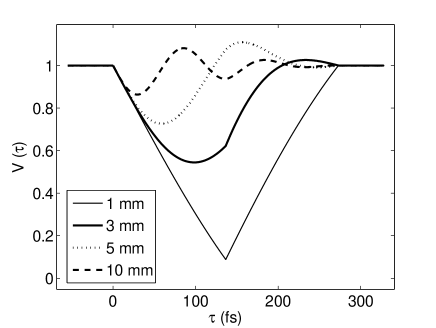
Figure 2: On the right side we can see the interference patterns with three different detector aperture sizes: the corresponding aperture functions are shown on the left side.

To get an analytic result one may assume Gaussian detection apertures of radius $R_{G}$ centered along the system’s optical axis:

$$p(\mathbf{x})=e^{-\frac{|\mathbf{x}|^{2}}{2R_{G}^{2}}}$$ (29)

In this case the solution is quite simple:

$$R(\tau)=R_{0}\left[1-\Lambda\left(1-\frac{2\tau}{DL}\right)e^{-\frac{\tau^{2}}{2\tau_{1}^{2}}}\right]$$ (30)

with:

$$\tau_{1}=\frac{2d_{1}D}{k_{p}MR_{G}}$$ (31)

Typically, sharp circular apertures are used in experiments. In this case, the function $\tilde{P}[\mathbf{q}]$ is described in terms of the Bessel function $J_{1}(x)$. For a circular aperture of radius $R$:

$$\tilde{P}[\mathbf{q}]=\frac{J_{1}(2R|\mathbf{q}|)}{R|\mathbf{q}|}$$ (32)

However the Gaussian approximation is still a good one if the width $R_{G}$ of the Gaussian is taken to roughly fit the Bessel function (of width $R$): in our case we take $R_{G}=R/(2\sqrt{2})$.
Therefore Eq. (30) is still approximately valid in the case of sharp circular apertures, just taking:

$$\tau_{1}=\frac{4\sqrt{2}d_{1}D}{k_{p}MR_{B}}$$ (33)

Mathematically, in Eq. (30) the interference pattern is given by the multiplication of a triangular function centered at $\tau=DL/2$ by a Gaussian function centered at $\tau=0$. The width of the Gaussian function $\tau_{1}$ decreases with increasing radius of the aperture $R_{B}$. Therefore, in the small aperture approximation, the width of the Gaussian is so large that it is approximately constant between $\tau=0$ and $\tau=DL/2$, giving the typical triangular dip found in quantum interference experiments. On the other hand, increasing the aperture size, the width of the Gaussian function decreases, reducing the dip visibility (see Fig. 2 ). Physically, this can be explained by the fact that increasing the aperture size we let more wave-vectors into the system, and so the spatial walk-off in type-II interferometry introduces distinguishability, reducing the interference visibility. Enlarging the aperture sizes is often useful in practice, for example to get a higher photon flux. Moreover, since in the SPDC process different frequency bands are emitted at different angles it may be necessary to open the detection aperture in applications where a broader bandwidth is needed. This is clearly a problem when using type-II phase matching in birefringent crystals, since the visibility of temporal and polarization interference gets drastically reduced.

III.2 Linear phase shift

Suppose now we introduce a linear phase function with the spatial light modulator, along the directon $\mathbf{s_{1}}$:

$$\varphi(\mathbf{x})=\mathbf{s_{1}}\cdot\mathbf{x}$$ (34)

we get:

$$\begin{split}W_{M}(\tau)&=\mbox{Sinc}\left[\frac{M^{2}Lk_{p}}{2d_{1}D}\tau\Lambda\left(1-\frac{2\tau}{DL}\right)\right]\\ &\tilde{P}_{A}\left[\frac{Mk_{p}}{2d_{1}D}\tau\mathbf{\hat{e}_{2}}+2f\mathbf{s_{1}}\right]\tilde{P}_{B}\left[-\frac{Mk_{p}}{2d_{1}D}\tau\mathbf{\hat{e}_{2}}-2f\mathbf{s_{1}}\right]\end{split}$$ (35)

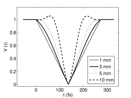
Figure 3: Quantum interference pattern for different detector aperture sizes, introducing a linear modulation of the deformable mirror, in order to restore the indistinguishability between the photons, decreased by the spatial walkoff in the generation process.

If we compare Eq. (35) with Eq. (30) we can see that the structure is the same; we again have a triangular function centered in $\tau=DL/2$, along with two aperture functions. But this time, instead of being centered at $\tau=0$, the aperture functions can be shifted at will along the $\tau$ axis. Suppose we now apply a tilt along the y axis ($s_{1x}=0$); the modulation function is then shifted to:

$$\tau_{center}=\frac{fD}{k_{0}M}s_{1y}$$ (36)

To get the highest possible visibility, the center of the modulation function must be matched to the center of the triangular dip:

$$\tau_{center}=\frac{DL}{2}$$ (37)

so that:

$$s_{1y}=\frac{k_{0}ML}{2f}$$ (38)

In the case of a reflective system, in which the phase modulation is implemented by means of a deformable mirror, tilted by an angle $\theta$:

$$\varphi(\mathbf{x})=2k_{0}\tan\theta y=s_{1y}y$$ (39)

Therefore, the amount of tilt necessary to restore high-visibility is:

$$\tan\theta=\frac{ML}{4f}$$ (40)

In the case of a 1.5 mm crystal, with M = 0.0723 (pump at 405 nm, SPDC at 810 nm) and lenses of focal length 20 cm in the 4-f system, we get:

$$\theta=0.14\;mrad$$ (41)

III.3 Large aperture approximation

If the detection apertures are large enough for the $\tilde{P}_{i}$ function to be successfully approximated by a delta-function we get:

$$W_{M}(\tau)=\int d\mathbf{q}G_{1}^{*}\left(\frac{f}{k_{0}}\mathbf{q}\right)G_{1}\left(-\frac{f}{k_{0}}\mathbf{q}\right)e^{i\frac{2Mk}{fD}\tau\mathbf{\hat{e}_{2}}\cdot\mathbf{q}}$$ (42)

Suppose that the spatial modulator is a circular aperture with radius r, with unit transmission and phase modulation described by the function $\varphi(\mathbf{x})$:

$$G_{1}(\mathbf{x})=\bigg{\{}\begin{array}[]{cc}0&\mbox{if $|\mathbf{x}|>r$}\\ e^{i\varphi(\mathbf{x})}&\mbox{if $|\mathbf{x}|<r$}\end{array}$$ (43)

In this case the function $\varphi(\mathbf{x})$ can be expanded on a set of polynomials which are orthogonal on the unit circle, like the Zernicke polynomials:

$$\begin{split}\varphi(\mathbf{q})&=\sum_{n}\sum_{m}\varphi_{nm}R_{n}^{m}(\rho)\cos(m\theta)\\ &\qquad\qquad(m=-n,-n+2,-n+4,...,n)\end{split}$$ (44)

where $\mathbf{q}=(\rho\cos\theta,\rho\sin\theta)$. To calculate $\varphi(-\mathbf{q})$ we note that $-\mathbf{q}=[\rho\cos(\theta+\pi),\rho\sin(\theta+\pi)]$, so:

$$\varphi(-\mathbf{q})=\sum_{n}\sum_{m}R_{n}^{m}(\rho)\cos[m(\theta+\pi)]$$ (45)

If m is even then $\cos[m(\theta+\pi)]=\cos(m\theta)$, otherwise if m is odd $\cos[m(\theta+\pi)]=-\cos m\theta)$. Therefore:

$$\varphi(\mathbf{q})-\varphi(-\mathbf{q})=2\sum_{n}\sum_{\mbox{m odd}}\varphi_{nm}R_{n}^{m}(\rho)\cos(m\theta)$$ (46)

So, only the Zernike polynomials with m odd contribute to the shape of the interference pattern. This effect is the spatial counterpart of the dispersion cancellation effect, in which only the odd-order terms in the Taylor expansion of the spectral phase survive. The experimental demonstration of this effect has been recently reported in Bonato et al. (2008)

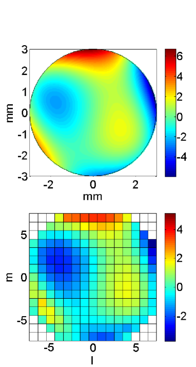
Figure 4: Example of the numerical approach adopted to evaluate Eq. (25) and Eq. (26). The spatial modulation surface is discretized in sufficiently small squares over which the phase is averaged.

IV Numerical solutions

Numerically solving for the quantities in Eq. (25) and Eq. (26) may be computationally demanding. Here, we propose an approximation, valid in the case where the function $G(\mathbf{x})$ changes smoothly over the mirror surface, as it is the case in experimentally relevant situations. This model is also interesting from the practical point of view, since in many cases adaptive optical systems are implemented using spatial light modulators or segmented deformable mirrors, where the modulation surface is partitioned into small pixels.

Suppose we partition the Fourier plane $\Pi_{F}$ into small squares (pixels) of side d. Let’s define the rectangular function:

$$\Pi(\mathbf{x})=\bigg{\{}\begin{array}[]{cc}0&\mbox{if $|\mathbf{x}|>\frac{1}{2}$}\\ 1&\mbox{if $|\mathbf{x}|<\frac{1}{2}$}\end{array}$$ (47)

The pixel (l, m) is identified by:

$$\sigma_{l,m}(x,y)=\Pi\left[\frac{x}{d}+l\right]\Pi\left[\frac{y}{d}+m\right]$$ (48)

selecting the area:

$$\left(l-\frac{1}{2}\right)d<x<\left(l+\frac{1}{2}\right)d$$

$$\left(m-\frac{1}{2}\right)d<y<\left(m+\frac{1}{2}\right)d$$ (49)

We approximate the value of the phase in each square by the mean value of the actual phase within the square:

$$\varphi_{lm}=\frac{1}{d^{2}}\int dxdy\varphi(x,y)\Pi\left[\frac{x}{d}+l\right]\Pi\left[\frac{y}{d}+m\right]$$ (50)

that is:

$$e^{i\varphi(x,y)}\approx\sum_{l,m}e^{i\varphi_{l,m}\Pi\left[\frac{x}{d}+l\right]\Pi\left[\frac{y}{d}+m\right]}$$ (51)

In this case (see Appendix B for a justification):

$$\sum_{l,m}e^{i\phi_{l,m}\Pi\left[\frac{x}{d}+l\right]\Pi\left[\frac{y}{d}+m\right]}=\sum_{l,m}e^{i\phi_{l,m}}\Pi\left[\frac{x}{d}+l\right]\Pi\left[\frac{y}{d}+m\right]$$ (52)

Substituting this expression in Eq. 23, and collecting the integrations one finds:

$$R(\tau)\approx\sum_{l,m}\sum_{\lambda,\mu}e^{-i\phi_{lm}-\phi_{\lambda,\mu}}\alpha_{l\lambda}I_{m\mu}(\tau)$$ (53)

where:

$$\begin{split}\alpha_{l\lambda}&=\int dq_{x}\int dQ_{x}\Pi\left[\frac{f}{kd}q_{x}-l\right]\Pi\left[\frac{f}{kd}Q_{x}-\lambda\right]\\ &\qquad\qquad\qquad e^{j\frac{2d_{1}}{k_{p}}(q_{x}^{2}-Q_{x}^{2})P[q_{x}+Q_{x}]P[-(q_{x}+Q_{x})]}\end{split}$$ (54)

and:

$$\begin{split}I_{m,\mu}(\tau)&=\int dq_{y}\int dQ_{y}\Pi\left[\frac{f}{kd}q_{y}-m\right]\Pi\left[\frac{f}{kd}Q_{y}-\mu\right]e^{j\frac{2d_{1}}{k_{p}}(q_{y}^{2}-Q_{y}^{2})}e^{-j\frac{M}{D}\tau(q_{y}-Q_{y})}\\ &\qquad\mbox{Sinc}\left[ML(q_{y}+Q_{y})\Lambda\left(1-\frac{2\tau}{DL}\right)\right]P[q_{y}+Q_{y}]P[-(q_{y}+Q_{y})]\end{split}$$ (55)

Performing the integrations one gets:

$$\alpha_{l\lambda}=\int dx\tilde{P}(x)\Lambda\left[\frac{fx}{kd}-(l+\lambda)\right]\mbox{sinc}\left\{\frac{2dd_{1}}{f}x\Lambda\left[\frac{fx}{kd}-(l+\lambda)\right]\right\}e^{i\frac{dd_{1}}{f}(l-\lambda)x}$$ (56)

and

$$\begin{split}I_{m\mu}(\tau)&=\int dx\tilde{P}(x)\Lambda\left[\frac{fx}{kd}-(m+\mu)\right]\mbox{sinc}\left\{MLx\Lambda\left[1-\frac{2\tau}{DL}\right]\right\}\\ &\qquad\mbox{sinc}\left\{\frac{2kd}{f}\left(\frac{2d_{1}}{k_{p}}x-\frac{M}{D}\tau\right)\Lambda\left[\frac{fx}{kd}-(m+\mu)\right]\right\}e^{i\frac{kd}{f}\left(\frac{2d_{1}}{k_{p}}x-\frac{M}{D}\tau\right)(m-\mu)}\end{split}$$ (57)

A similar expression can be found for the background coincidence rate:

$$R_{0}\approx\sum_{l,m}\sum_{\lambda,\mu}e^{-i(\phi_{lm}-\phi_{\lambda,\mu})}R^{(x)}_{l\lambda}R^{(y)}_{m\mu}$$ (58)

where:

$$\begin{split}R^{(x)}_{l\lambda}&=\int dx\tilde{P}(x)\Lambda\left[\frac{fx}{kd}-(l-\lambda)\right]\\ &\qquad\mbox{sinc}\left\{\frac{2dd_{1}}{f}x\Lambda\left[\frac{fx}{kd}-(l-\lambda)\right]\right\}e^{i\frac{dd_{1}}{f}(l+\lambda)x}\end{split}$$ (59)

and

$$\begin{split}R^{(y)}_{m\mu}&=\int dx\tilde{P}(x)\Lambda\left[\frac{fx}{kd}-(m-\mu)\right]\mbox{sinc}\left(MLx\right)\\ &\qquad\mbox{sinc}\left\{\frac{2dd_{1}}{f}x\Lambda\left[\frac{fx}{kd}-(m-\mu)\right]\right\}e^{i\left[\frac{dd_{1}}{f}(m+\mu)-\frac{ML}{2}\right]x}\end{split}$$ (60)

The advantage of our numerical approach is that one can calculate and tabulate the functions $R^{(x)}_{l\lambda}$, $R^{(y)}_{m\mu}$, $\alpha_{l\lambda}$ and $I_{m\mu}(\tau)$ for a given configuration, determined by the focal length f, the shape of the detection apertures, the width of the deformable optics and the distance between the crystal and the detectors. Then, to calculate the shape of the interference pattern for a certain phase distribution on the adaptive optics one just needs to change the coefficient of a linear combination of the tabulated functions. This can be a helpful tool to study the effect of specific aberrations on the temporal interference or to engineer the shape of the HOM dip.

In the limit of large detector apertures $\tilde{P}(x)\approx\delta(x)$:

$$\alpha_{l\lambda}=\delta(l+\lambda)$$ (61)

$$I_{m\mu}=\mbox{sinc}\left[\frac{2kdM}{fD}\tau\right]e^{-i\frac{2kdM}{fD}m\tau}\delta(m+\mu)$$ (62)

So:

$$R_{BIG}(\tau)\approx\sum_{l,m}e^{-i(\varphi_{lm}-\varphi_{-l,-m})}\alpha_{l,-l}I_{m,-m}(\tau)$$ (63)

We have a discrete formulation of the even-order spatial phase cancellation effect. What affects the shape of the dip is the difference between the phase of the pixel (l, m) and the phase of the pixel symmetric to it with respect to the origin (-l, -m). Therefore, since for even functions $\phi_{lm}=\phi_{-l,-m}$, the phase difference is zero and they do not contribute to the coincidentce pattern. This way our approximate solution technique is consistent with the general theory.

V Discussion

V.1 Examples

According to Eq. 23, the shape of the temporal quantum interference pattern is affected by the spatial modulation given by the deformable mirror. In Section IV we proposed a numerical approach to calculate easily the shape of the temporal interferogram. For example, some results are reported in Fig. 5, for coma (upper plot) and a superposition of several different aberrations (lower plot). The interference visibility clearly degrades in presence of wave-front aberrations.

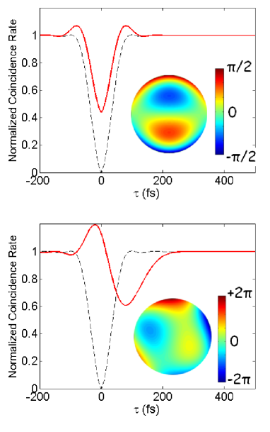
Figure 5: Examples of the shape of the polarization quantum-interference dip with two different spatial phase modulations (in black the unperturbed dip, in red the modulated one). In the upper figure the effect of a small amount of coma along the vertical axis is shown. In the lower figure a more complicated superposition of aberrations affects dramatically the shape of the dip

V.2 Limits and role of the large aperture approximation

An interesting question is under what experimental conditions the large aperture approximation can be considered to be valid, so as to obtain the even-order aberration cancellation effect.

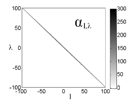
Figure 6: Plot of the values of $|\alpha_{l,\lambda}|^{2}$, for $l,\lambda=-100...+100$. The radius of the detection apertures is $R=5$ mm, the distance between the exit plane of the modulation section and the detection apertures is $d-1=1$ m and the size of the modulation pixels is $d=25\mu$m. Clearly only the diagonal elements contribute are non-zero, i.e. the ones for which $\lambda=-l$. In this situation the effect of even-order aberration cancellation is present.

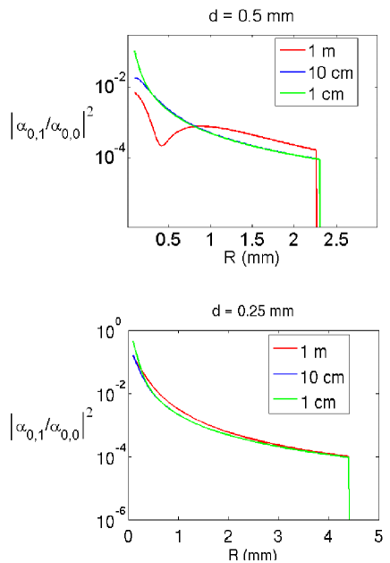
Figure 7: Plot of the ratio $\rho_{0}$ between the intensities of the non-diagonal coefficient $\alpha_{01}$ and the diagonal coefficient $\alpha_{00}$ as a function of the radius of Gaussian detection apertures $R$, for different values of the distance between the exit plane of the modulation section and the detection apertures ($d_{1}=1,10,100$ cm). On the upper plot the size of the modulation pixel $d$ is $d=0.5$ mm, while in the second case it is $d=0.25$ mm. Clearly, for experimentally interesting cases, the off-diagonal coefficient is at least 3 orders of magnitude smaller than the diagonal one, leading to even-order aberration cancellation.

According to the numerical approach proposed in Section IV, the even-order aberration cancellation effect manifests itself in the limit where, for example:

$$\alpha_{l,\lambda}\rightarrow\delta(l+\lambda)$$ (64)

In Fig. 6, a plot of the value for $\alpha_{l,\lambda}$ is shown for typical values of the relevant experimental parameters (detection aperture radius $R=5$ mm, detection distance $d_{1}=1$ m and size $d=0.1$ mm of each pixel in the Fourier plane of the adaptive optical system). Clearly, only the diagonal elements (the ones for which $l=-\lambda$ are significant), suggesting that the effect of even-order aberration cancellation may be observable for most typical experimental parameters.

To get an idea of what happens for different experimental conditions we can compute the ratio between the intensities of the non-diagonal coefficient $\alpha_{01}$ and the diagonal coefficient $\alpha_{00}$:

$$\rho_{0}=\frac{|\alpha_{01}|^{2}}{|\alpha_{00}|^{2}}$$ (65)

The lower the value for $\rho_{0}$ the less significant the coefficients for $\lambda\neq-l$ are: the even-order aberration cancellation effect will therefore manifest itself more clearly.

Values for $\rho_{0}$ are shown in Fig. 7 for two different cases. In both pictures, the value of $\rho_{0}$ is shown as a function of the Gaussian detection aperture radius $R$, for three different values of the distance between the plane $\Pi_{3}$ and the detection lenses $d_{1}$. In the upper figure, the size of each small square in which the spatial phase is assumed to be constant is $d=0.5$ mm, while in the second case it is $d=0.25$ mm. In both cases $\rho_{0}$ is significantly smaller than 1, and it becomes smaller and smaller increasing the value of the detection aperture radius. However, $\rho_{0}$ is smaller for larger values of $d$, implying that the spatial variability of the modulation phase plays a role in the degree of even-order cancellation of the modulation itself.

It turns out that for the aberration cancellation effect to appear, it is in fact only necessary for one aperture to be large and for one detector to be integrated over. This is sufficient to produce the transverse-momentum delta functions that lead to even-order cancellation. To demonstrate this, we can for example consider the case where the aperture at $B$ is large, and the detector at $B$ is integrated over, while the aperture at $A$ is taken to be finite, with detector $A$ treated as pointlike. The location of the pointlike detector will henceforth simply be denoted as $x$, and we continue to work within the quasi-monochromatic approximation. If we integrate only over $x_{B}$, leaving $x$ unintegrated, then it is straightforward to show that:

$$W^{(0)} =\;e^{{icd}\over{\Omega_{0}}}$$

$$\times\left\{\tilde{Q}\left(q+{{\Omega_{0}x}\over{cf_{0}}}\right)\tilde{Q}^{\prime}\left(-q^{\prime}-{{\Omega_{0}x}\over{cf_{0}}}\right)\tilde{P}_{B}\left(q^{\prime}-q\right)\right.$$

$$+\left.\tilde{Q}\left(-q+{{\Omega_{0}x}\over{cf_{0}}}\right)\tilde{Q}^{\prime}\left(q^{\prime}-{{\Omega_{0}x}\over{cf_{0}}}\right)\tilde{P}_{B}\left(q-q^{\prime}\right)\right\}$$

$$W_{M} =\;e^{{icd}\over{\Omega_{0}}}$$

$$\times\left\{\tilde{Q}\left(q+{{\Omega_{0}x}\over{cf_{0}}}\right)\tilde{Q}^{\prime}\left(-q^{\prime}+{{\Omega_{0}x}\over{cf_{0}}}\right)\tilde{P}_{B}\left(-q^{\prime}+q\right)\right.$$

$$+\left.\tilde{Q}\left(-q+{{\Omega_{0}x}\over{cf_{0}}}\right)\tilde{Q}^{\prime}\left(+q^{\prime}+{{\Omega_{0}x}\over{cf_{0}}}\right)\tilde{P}_{B}\left(q-q^{\prime}\right)\right\}$$

Here, we have defined $\tilde{Q}$ and $\tilde{Q}^{\prime}$ to be the Fourier transforms respectively of $p_{A}$ and $p_{A}^{\ast}$. $\tilde{P}_{B}$ is, as before, the Fourier transform of $|p_{B}|^{2}$. We now let aperture $B$ become large, so that the function $\tilde{P}_{B}$ goes over to a delta function. For $G_{1}(x)=e^{i\phi(x)}$ and $G_{2}(x)=1$, we can substitute these results into the coincidence rate (which will now be a function of both $\tau$ and the position $x$ of detector $A$), and carry out the $q^{\prime}$ and $\nu$ integrals. For the modulation term, we find:

$$R_{M}(x,\tau) = R(x,\tau)-R_{0}(x)$$ (68)

$$= \int dq\;e^{i[\phi(q)-\phi(-q)]}$$

$$\times e^{{{2iM\tau}\over D}{\mathbf{e_{2}}\cdot\mathbf{q}}}e^{{{2iq^{2}}\over{k_{p}}}\left[{{2\tau}\over D}+L\right]}\mbox{Sinc}\left({{2q^{2}L}\over{k_{p}}}\right)$$

$$\times\left[\tilde{Q}\left(q+{{{\Omega_{0}x}\over{cf_{0}}}}\right)\tilde{Q}^{\ast}\left(-q-{{{\Omega_{0}x}\over{cf_{0}}}}\right)\right.$$

$$+\left.\tilde{Q}\left(-q+{{{\Omega_{0}x}\over{cf_{0}}}}\right)\tilde{Q}^{\ast}\left(q-{{{\Omega_{0}x}\over{cf_{0}}}}\right)\right].$$

Here, we have used the fact that the Fourier transform of $p_{A}^{\ast}(x)$ equals the complex conjugate of the Fourier transform of $p_{A}(x)$, in order to write $\tilde{Q}^{\prime}$ in terms of $\tilde{Q}$. We see from the presence of the factor $e^{i[\phi(q)-\phi(-q)]}$ that even-order aberration cancellation occurs even though one aperture is finite and the corresponding detector is pointlike. This point may be of importance in future attempts to produce aberration free imaging.

VI Conclusions

Summarizing, we have in this paper done a theoretical study of the relation between the wavelength modulation of the entangled SPDC photons and the shape of the resulting temporal quantum interference pattern. Due to the multiparametric nature of the generated entangled states, the modulation on the spatial degree of freedom can affect the shape of the polarization-temporal interference pattern in the coincidence rate. Our aim is twofold: from one side we want to study the effect of wavefront aberration on quantum interferometry, from the other we want to discuss a way to engineer multiparametrically-entangled states.

We have introduced a theoretical model to calculate the shape of the polarization-temporal interference pattern given a certain phase modulation in the crystal far-field, assuming as a free parameter the shape and the dimension of the collection apertures. Using a numerical method to study the resulting equation has shown that for typical experimental cases the hypothesis of large apertures can be assumed valid. In such an approximation, only the odd part of the assigned phase modulation affects the shape of the interference pattern. This effect has recently been demonstrated experimentally Bonato et al. (2008).

Moreover, it is often useful in experiments to enlarge the collection aperture in order to collect a higher photon flux and larger optical bandwidth. But when working with type-II birefringently phase-matched downconversion, spatial walk-off between the emitted photons introduces distinguishability between the two possible events that can lead to coincidence detection, reducing the visibility of quantum interference. Such walk-off can be compensated with a linear phase shift in the vertical direction, restoring high visibility.

Appendix A Derivation of Eq. 23

In this Appendix we sketch the major steps for the derivation of Eq. (23). Substituting Eq. (21) into Eq. (16), and the result into Eq. (22) one finds the following expressions for $R_{0}$ and $W_{G}(\tau)$:

$$\begin{split}R_{0}&=\int d\mathbf{q}d\mathbf{q^{\prime}}d\nu\Phi^{*}(\mathbf{q},\nu)\Phi(\mathbf{q^{\prime}},\nu)G_{1}^{*}\left(\frac{f}{k}\mathbf{q}\right)G_{1}\left(\frac{f}{k}\mathbf{q^{\prime}}\right)\\ &\qquad\quad\times G_{2}^{*}\left(\frac{f}{k}\mathbf{q}\right)G_{2}\left(\frac{f}{k}\mathbf{q^{\prime}}\right)W^{(0)}(\mathbf{q},\mathbf{q^{\prime}},\nu)\end{split}$$ (70)

$$\begin{split}W_{M}(\tau)&=\frac{1}{R_{0}}\int d\mathbf{q}d\mathbf{q^{\prime}}d\nu\Phi^{*}(\mathbf{q},\nu)\Phi(\mathbf{q^{\prime}},-\nu)G_{1}^{*}\left(\frac{f}{k}\mathbf{q}\right)\\ &\times G_{1}\left(\frac{f}{k}\mathbf{q^{\prime}}\right)G_{2}^{*}\left(\frac{f}{k}\mathbf{q}\right)G_{2}\left(\frac{f}{k}\mathbf{q^{\prime}}\right)W(\mathbf{q},\mathbf{q^{\prime}},\nu)\end{split}$$ (71)

where:

$$\begin{split}W^{(0)}(\mathbf{q},\mathbf{q^{\prime}},\nu)&=\int d\mathbf{x_{A}}d\mathbf{x_{B}}H^{*}(\mathbf{x_{A}},\mathbf{q},\nu)H^{*}(\mathbf{x_{B}},-\mathbf{q},-\nu)H(\mathbf{x_{A}},\mathbf{q^{\prime}},\nu)H(\mathbf{x_{B}},-\mathbf{q^{\prime}},-\nu)\\ &\qquad\qquad+H^{*}(\mathbf{x_{A}},-\mathbf{q},-\nu)H^{*}(\mathbf{x_{B}},\mathbf{q},\nu)H(\mathbf{x_{A}},-\mathbf{q^{\prime}},-\nu)H(\mathbf{x_{B}},\mathbf{q^{\prime}},\nu)\end{split}$$ (72)

and

$$\begin{split}W(\mathbf{q},\mathbf{q^{\prime}},\nu)&=\int d\mathbf{x_{A}}d\mathbf{x_{B}}H^{*}(\mathbf{x_{A}},\mathbf{q},\nu)H^{*}(\mathbf{x_{B}},-\mathbf{q},-\nu)H(\mathbf{x_{A}},-\mathbf{q^{\prime}},\nu)H(\mathbf{x_{B}},\mathbf{q^{\prime}},-\nu)\\ &\qquad\qquad+H^{*}(\mathbf{x_{A}},-\mathbf{q},-\nu)H^{*}(\mathbf{x_{B}},\mathbf{q},\nu)H(\mathbf{x_{A}},\mathbf{q^{\prime}},-\nu)H(\mathbf{x_{B}},-\mathbf{q^{\prime}},\nu)\end{split}$$ (73)

The angular and spectral emission function $\Phi(\mathbf{q},\nu)$ is given by:

$$\Phi(\mathbf{q},\nu)=\int dz\quad\Pi\left[\frac{z}{L}+\frac{1}{2}\right]e^{-i\Delta(\mathbf{q},\nu)z}$$ (74)

Performing the integrals over the spatial coordinates $d\mathbf{x_{A}}$ and $\mathbf{x_{B}}$ one gets:

$$\begin{split}W^{(0)}(\mathbf{q},\mathbf{q^{\prime}},\nu)&=e^{i\frac{2d_{1}}{k_{p}}[|\mathbf{q}|^{2}-|\mathbf{q^{\prime}}|^{2}]}\tilde{P}_{A}[(\mathbf{q}-\mathbf{q^{\prime}})]\tilde{P}_{B}[-(\mathbf{q}-\mathbf{q^{\prime}})]\\ &\qquad\qquad+\tilde{P}_{A}[-(\mathbf{q}-\mathbf{q^{\prime}})]\tilde{P}_{B}[(\mathbf{q}-\mathbf{q^{\prime}})]\end{split}$$ (75)

and

$$\begin{split}W(\mathbf{q},\mathbf{q^{\prime}},\nu)&=e^{i\frac{2d_{1}}{k_{p}}[|\mathbf{q}|^{2}-|\mathbf{q^{\prime}}|^{2}]}\tilde{P}_{A}[(\mathbf{q}+\mathbf{q^{\prime}})]\tilde{P}_{B}[-(\mathbf{q}+\mathbf{q^{\prime}})]+\\ &\qquad\qquad\tilde{P}_{A}[-(\mathbf{q}+\mathbf{q^{\prime}})]\tilde{P}_{B}[(\mathbf{q}+\mathbf{q^{\prime}})]\end{split}$$ (76)

Finally, use of the integral representation for the sinc function (Eq. (74)) allows the $\nu$ integration to be carried out, but at the expense of introducing two integrations over a pair of new parameters (say $z$ and $z^{\prime}$). Note the relation

$$\Pi[x]\Pi[x-\alpha]=\left\{\begin{array}[]{ll}1&,\mbox{ if }-1\leq\alpha\leq 0,\;-{1\over 2}\leq x\leq{1\over 2}+\alpha\\ 1&,\mbox{ if }0\leq\alpha\leq 1,\;-{1\over 2}+\alpha\leq x\leq{1\over 2}\\ 0&,\mbox{ else .}\end{array}\right.$$ (77)

From this, it follows that

$$\int\Pi[x]\Pi[x-\alpha]dx=\Lambda(\alpha),$$ (78)

where $\Lambda(\alpha)$ is the triangle function. These facts allow us to carry out the two z-integrations that arise from the sinc function, leading to the result shown in Eq. (23).

Appendix B Justification of Eq. (52)

Suppose to have a set $A$, which can be partitioned into a collection of disjoint subsets $A_{k},k=1,2,...$:

$$\bigcup_{k}A_{k}=A\qquad A_{k}\cap A_{l}=\phi\quad\mbox{if}\quad k\neq l$$ (79)

To each set we can associate a characteristic function:

$$\chi_{k}(x)=\bigg{\{}\begin{array}[]{c}1,\qquad x\in A_{k}\\ 0,\qquad x\notin A_{k}\end{array}$$ (80)

such that:

$$\sum_{k}\chi_{k}(x)=\chi_{A}(x),\qquad\chi_{k}(x)\chi_{l}(x)=\delta_{kl}\chi_{k}(x),$$ (81)

where $\chi_{A}$ is the characteristic function for the full set,

$$\chi_{A}(x)=\bigg{\{}\begin{array}[]{c}1,\qquad x\in A\\ 0,\qquad x\notin A\end{array}$$ (82)

The term $e^{i\phi_{k}\chi_{k}(x)}$ assumes the value $e^{i\phi_{k}}$ for $\chi_{k}(x)=1$ and the value $1$ for $\chi_{k}(x)=0$ ($1-\chi_{k}(x)=1$), so:

$$\begin{split}e^{i\sum_{k}\phi_{k}\chi_{k}(x)}&=\prod_{k}e^{i\phi_{k}\chi_{k}(x)}\\ &=\prod_{k}\left[1\cdot(1-\chi_{k}(x))+e^{i\phi_{k}}\cdot\chi_{k}(x)\right]\\ &=\prod_{k}\left[1+(e^{i\phi_{k}}-1)\chi_{k}\right]\end{split}$$ (83)

If we express the first few terms we get:

$$\begin{split}\prod_{k}&\left[1+(e^{i\phi_{k}}-1)\chi_{k}\right]=\\ &=\left[1+(e^{i\phi_{1}}-1)\chi_{1}\right]\left[1+(e^{i\phi_{2}}-1)\chi_{2}\right]...\\ &=1+(e^{i\phi_{1}}-1)\chi_{1}+(e^{i\phi_{2}}-1)\chi_{2}+...\\ &\qquad+(e^{i\phi_{1}}-1)(e^{i\phi_{2}}-1)\chi_{1}\chi_{2}+\\ &+(e^{i\phi_{1}}-1)(e^{i\phi_{3}}-1)\chi_{1}\chi_{3}+....\\ &\qquad+(e^{i\phi_{1}}-1)(e^{i\phi_{1}}-1)(e^{i\phi_{1}}-1)\chi_{1}\chi_{2}\chi_{3}\\ &\qquad\quad+(e^{i\phi_{1}}-1)(e^{i\phi_{2}}-1)(e^{i\phi_{4}}-1)\chi_{1}\chi_{2}\chi_{4}+...\end{split}$$ (84)

So that in the end:

$$\begin{split}e^{i\sum_{k}\phi_{k}\chi_{k}(x)}&=1+\sum_{k}\left[\left(e^{i\phi_{k}}-1\right)\chi_{k}\right]\\ &=1+\sum_{k}e^{i\phi_{k}}\chi_{k}-\sum_{k}\chi_{k}\\ &=\sum_{k}e^{i\phi_{k}}\chi_{k}\end{split}$$ (85)

Since the square sets we have used in section IV satisfy Eq. (B1), then the result expressed in Eq. (B5) is valid for our case.

References

- Schroedinger (1935) E. Schroedinger, Naturwissenschaften 23, 807 (1935).
- Klyshko (1967) D. N. Klyshko, JETP Letters 6, 23 (1967).
- Harris et al. (1967) S. E. Harris, M. K. Osham, and R. L. Byer, Phys. Rev. Lett. 18, 732 (1967).
- Giallorenzi and Tang (1968) T. G. Giallorenzi and C. L. Tang, Phys. Rev. 166, 225 (1968).
- Kleinmann (1968) D. A. Kleinmann, Phys. Rev. 174, 1027 (1968).
- Atature et al. (2002) M. Atature, G. D. Giuseppe, M. Shaw, A. V. Sergienko, B. E. A. Saleh, and M. C. Teich, Phys. Rev. A 66, 023822 (2002).
- Abouraddy et al. (2002) A. Abouraddy, M. B. Nasr, B. E. A. Saleh, A. V. Sergienko, and M. C. Teich, Phys. Rev. A 65, 053817 (2002).
- Nasr et al. (2003) M. B. Nasr, B. E. A. Saleh, A. V. Sergienko, and M. C. Teich, Phys. Rev. Lett. 91, 083601 (2003).
- Franson (1995) J. D. Franson, Phys. Rev. A 45, 3126 (1995).
- Steinberg et al. (1992) A. M. Steinberg, P. G. Kwiat, and R. Y. Chiao, Phys. Rev. A 45, 6659 (1992).
- Bonato et al. (2008) C. Bonato, A. V. Sergienko, B. E. A. Saleh, S. Bonora, and P. Villoresi (2008), arXiv:0807.2909.
- Rubin (1996) M. H. Rubin, Phys. Rev. A 54, 5349 (1996).
- Goodman (1996) J. W. Goodman, Introduction to Fourier Optics (McGraw-Hill, 1996), 2nd ed.