Large Scale Variational Inference and Experimental Design for Sparse Generalized Linear Models

Abstract

Many problems of low-level computer vision and image processing, such as denoising, deconvolution, tomographic reconstruction or super-resolution, can be addressed by maximizing the posterior distribution of a sparse linear model (SLM). We show how higher-order Bayesian decision-making problems, such as optimizing image acquisition in magnetic resonance scanners, can be addressed by querying the SLM posterior covariance, unrelated to the density’s mode. We propose a scalable algorithmic framework, with which SLM posteriors over full, high-resolution images can be approximated for the first time, solving a variational optimization problem which is convex iff posterior mode finding is convex. These methods successfully drive the optimization of sampling trajectories for real-world magnetic resonance imaging through Bayesian experimental design, which has not been attempted before. Our methodology provides new insight into similarities and differences between sparse reconstruction and approximate Bayesian inference, and has important implications for compressive sensing of real-world images. Parts of this work appeared at conferences [33, 22].

1 Introduction

Natural images have a sparse low-level statistical signature, represented in the prior distribution of a sparse linear model (SLM). Imaging problems such as reconstruction, denoising or deconvolution can successfully be solved by maximizing its posterior density (maximum a posteriori (MAP) estimation), a convex program for certain SLMs, for which efficient solvers are available. The success of these techniques in modern imaging practice has somewhat shrouded their limited scope as Bayesian techniques: of all the information in the posterior distribution, they make use of the density’s mode only.

Consider the problem of optimizing image acquisition, our major motivation in this work. Magnetic resonance images are reconstructed from Fourier samples. With scan time proportional to the number of samples, a central question to ask is which sampling designs of minimum size still lead to MAP reconstructions of diagnostically useful image quality? This is not a direct reconstruction problem, the focus is on improving measurement designs to better support subsequent reconstruction. Goal-directed acquisition optimization cannot sensibly be addressed by MAP estimation, yet we show how to successfully drive it by Bayesian posterior information beyond the mode. Advanced decision-making of this kind needs uncertainty quantification (posterior covariance) rather than point estimation, requiring us to step out of the sparse reconstruction scenario and approximate sparse Bayesian inference instead.

The Bayesian inference relaxation we focus on is not new [11, 23, 17], yet when it comes to problem characterization or efficient algorithms, previous inference work lags far behind standards established for MAP reconstruction. Our contributions range from theoretical characterizations over novel scalable solvers to applications not previously attempted. The inference relaxation is shown to be a convex optimization problem if and only if this holds for MAP estimation (Section 3), a property not previously established for this or any other SLM inference approximation. Moreover, we develop novel scalable double loop algorithms to solve the variational problem orders of magnitude faster than previous methods we are aware of (Section 4). These algorithms expose an important link between variational Bayesian inference and sparse MAP reconstruction, reducing the former to calling variants of the latter few times, interleaved by Gaussian covariance (or PCA) approximations (Section 4.4). By way of this reduction, the massive recent interest in MAP estimation can play a role for variational Bayesian inference just as well. To complement these similarities and clarify confusion in the literature, we discuss computational and statistical differences of sparse estimation and Bayesian inference in detail (Section 5).

The ultimate motivation for novel developments presented here is sequential Bayesian experimental design (Section 6), applied to acquisition optimization for medical imaging. We present a powerful variant of adaptive compressive sensing, which succeeds on real-world image data where theoretical proposals for non-adaptive compressive sensing [9, 6, 10] fail (Section 6.1). Among our experimental results is part of a first successful study for Bayesian sampling optimization of magnetic resonance imaging, learned and evaluated on real-world image data (Section 7.4).

An implementation of the algorithms presented here is publicly available, as part of the glm-ie toolbox (Section 4.6). It can be downloaded from mloss.org/software/view/269/.

2 Sparse Bayesian Inference. Variational Approximations

In a sparse linear model (SLM), the image $\bm{u}\in\mathbb{R}^{n}$ of $n$ pixels is unknown, and $m$ linear measurements $\bm{y}\in\mathbb{R}^{m}$ are given, where $m\ll n$ in many situations of practical interest.

$$\bm{y}=\bm{X}\bm{u}+\bm{\mathrm{\varepsilon}},\quad\bm{\mathrm{\varepsilon}}\sim N(\bm{0},\sigma^{2}\bm{I}),$$ (1)

where $\bm{X}\in\mathbb{R}^{m\times n}$ is the design matrix, and $\bm{\mathrm{\varepsilon}}$ is Gaussian noise of variance $\sigma^{2}$, implying the Gaussian likelihood $P(\bm{y}|\bm{u})=N(\bm{y}|\bm{X}\bm{u},\sigma^{2}\bm{I})$. Natural images are characterized by histograms of simple filter responses (derivatives, wavelet coefficients) exhibiting super-Gaussian (or sparse) form: most coefficients are close to zero, while a small fraction have significant sizes [35, 28] (a precise definition of super-Gaussianity is given in Section 2.1). Accordingly, SLMs have super-Gaussian prior distributions $P(\bm{u})$. The MAP estimator $\hat{\bm{u}}_{\text{MAP}}:=\operatorname*{argmax}_{\bm{u}}[\log P(\bm{y}|\bm{u})+\log P(\bm{u})]$ can outperform maximum likelihood $\hat{\bm{u}}_{\text{ML}}:=\operatorname*{argmax}_{\bm{u}}\log P(\bm{y}|\bm{u})$, when $\bm{u}$ represents an image.

In this paper, we focus on priors of the form $P(\bm{u})\propto\prod_{i=1}^{q}t_{i}(s_{i})$, where $\bm{s}=\bm{B}\bm{u}$. The potential functions $t_{i}(\cdot)$ are positive and bounded. The operator $\bm{B}\in\mathbb{R}^{q\times n}$ may contain derivative filters or a wavelet transform. Both $\bm{X}$ and $\bm{B}$ have to be structured or sparse, in order for any SLM algorithm to be scalable. Laplace (or double exponential) potentials are sparsity-enforcing:

$$t_{i}(s_{i})=e^{-\tau_{i}|s_{i}|},\quad\tau_{i}>0.$$ (2)

For this particular prior and the Gaussian likelihood (1), MAP estimation corresponds to a quadratic program, known as LASSO [37] for $\bm{B}=\bm{I}$. Note that $\log t_{i}(s_{i})$ is concave. In general, if log-concavity holds for all model potentials, MAP estimation is a convex problem. Another example for sparsity potentials are Student’s t:

$$t_{i}(s_{i})=(1+(\tau_{i}/\nu)s_{i}^{2})^{-(\nu+1)/2},\quad\tau_{i},\nu>0.$$ (3)

For these, $\log t_{i}(s_{i})$ is not concave, and MAP estimation is not (in general) a convex program. Note that $-\log t_{i}(s_{i})$ is also known as Lorentzian penalty function.

2.1 Variational Lower Bounds

Bayesian inference amounts to computing moments of the posterior distribution

$$\begin{split}P(\bm{u}|\bm{y})&=Z^{-1}N(\bm{y}|\bm{X}\bm{u},\sigma^{2}\bm{I})\prod\nolimits_{i=1}^{q}t_{i}(s_{i}),\quad\bm{s}=\bm{B}\bm{u},\\ Z&=\int N(\bm{y}|\bm{X}\bm{u},\sigma^{2}\bm{I})\prod\nolimits_{i=1}^{q}t_{i}(s_{i})\,d\bm{u}.\end{split}$$ (4)

This is not analytically tractable in general for sparse linear models, due to two reasons coming together: $P(\bm{u}|\bm{y})$ is highly coupled ($\bm{X}$ is not blockdiagonal) and non-Gaussian. We focus on variational approximations here, rooted in statistical physics. The log partition function $\log Z$ (also known as log evidence or log marginal likelihood) is the prime target for variational methods [42]. Formally, the potentials $t_{i}(s_{i})$ are replaced by Gaussian terms of parametrized width, the posterior $P(\bm{u}|\bm{y})$ by a Gaussian approximation $Q(\bm{u}|\bm{y})$. The width parameters are adjusted by fitting $Q(\bm{u}|\bm{y})$ to $P(\bm{u}|\bm{y})$, in what amounts to the variational optimization problem.

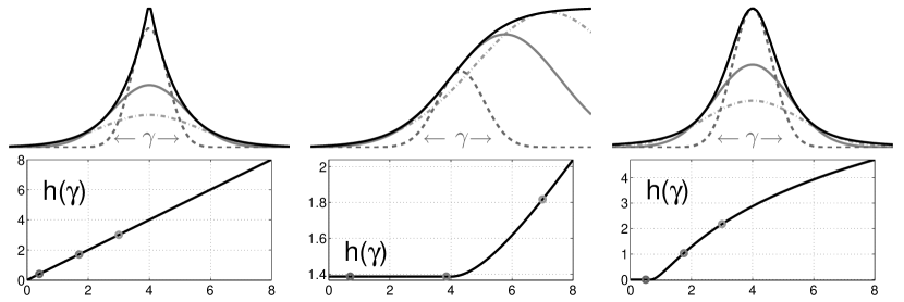
Figure 1: Super-Gaussian distributions admit tight Gaussian-form lower bounds of any width $\gamma$. Left: Laplace (2); middle: Bernoulli (6); right: Student’s t (3).

Our variational relaxation exploits the fact that all potentials $t_{i}(s_{i})$ are (strongly) super-Gaussian: there exists a $b_{i}\in\mathbb{R}$ such that $\tilde{g}_{i}(s_{i}):=\log t_{i}(s_{i})-b_{i}s_{i}$ is even, and convex and decreasing as a function of $x_{i}:=s_{i}^{2}$ [23]. We write $g_{i}(x_{i}):=\tilde{g}_{i}(x_{i}^{1/2})$, $x_{i}\geq 0$ in the sequel. This implies that

$$t_{i}(s_{i})=\max_{\gamma_{i}\geq 0}e^{b_{i}s_{i}-s_{i}^{2}/(2\gamma_{i})-h_{i}(\gamma_{i})/2},\quad h_{i}(\gamma_{i}):=\max_{x_{i}\geq 0}(-x_{i}/\gamma_{i}-2g_{i}(x_{i})).$$ (5)

A super-Gaussian $t_{i}(s_{i})$ has tight Gaussian-form lower bounds of all widths (see Figure 1). We replace $t_{i}(s_{i})$ by these lower bounds in order to step from $P(\bm{u}|\bm{y})$ to the family of approximations $Q(\bm{u}|\bm{y})\propto P(\bm{y}|\bm{u})e^{\bm{b}^{T}\bm{s}-\frac{1}{2}\bm{s}^{T}(\operatorname{diag}\bm{\gamma})^{-1}\bm{s}}$, where $\bm{\gamma}=(\gamma_{i})$.

To establish (5), note that the extended-value function $g_{i}(x_{i})$ (assigning $g_{i}(x_{i})=\infty$ for $x_{i}<0$) is a closed proper convex function, thus can be represented by Fenchel duality [26, Sect. 12]: $g_{i}(x_{i})=\sup_{\lambda_{i}}x_{i}\lambda_{i}-g_{i}^{*}(\lambda_{i})$, where the conjugate function $g_{i}^{*}(\lambda_{i})=\sup_{x_{i}}x_{i}\lambda_{i}-g_{i}(x_{i})$ is closed convex as well. For $x_{i}\geq 0$ and $\lambda_{i}>0$, we have that $x_{i}\lambda_{i}-g_{i}(x_{i})\geq x_{i}\lambda_{i}-g_{i}(0)\to\infty$ with $x_{i}\to\infty$, which implies that $g_{i}^{*}(\lambda_{i})=\infty$ for $\lambda_{i}>0$. Also, $g_{i}^{*}(0)=-\lim_{x_{i}\to\infty}g_{i}(x_{i})$, so that $-g_{i}^{*}(0)<g_{i}(x_{i})$ for any $x_{i}<\infty$. Therefore, for any $x_{i}\in[0,\infty)$, $g_{i}(x_{i})=\sup_{\lambda_{i}<0}x_{i}\lambda_{i}-g_{i}^{*}(\lambda_{i})$. Reparameterizing $\gamma_{i}:=-1/(2\lambda_{i})$, we have that $g_{i}(x_{i})=\max_{\gamma_{i}\geq 0}-x_{i}/(2\gamma_{i})-g_{i}^{*}(-1/(2\gamma_{i}))$ (note that in order to accommodate $g_{i}(0)$ in general, we have to allow for $\gamma_{i}=0$). Finally, $h_{i}(\gamma_{i}):=2g_{i}^{*}(-1/(2\gamma_{i}))$.

The class of super-Gaussian potentials is large. All scale mixtures (mixtures of zero-mean Gaussians $t_{i}(s_{i})=\mathrm{E}_{\gamma_{i}}[N(s_{i}|0,\gamma_{i})]$) are super-Gaussian, and $h_{i}(\gamma_{i})$ can be written in terms of the density for $\gamma_{i}$ [23]. Both Laplace (2) and Student’s t potentials (3) are super-Gaussian, with $h_{i}(\gamma_{i})$ given in Appendix A.6. Bernoulli potentials, used as binary classification likelihoods,

$$t_{i}(s_{i})=\left(1+e^{-y_{i}\tau_{i}s_{i}}\right)^{-1},\quad y_{i}\in\{\pm 1\},\;\tau_{i}>0$$ (6)

are super-Gaussian, with $b_{i}=y_{i}\tau_{i}/2$ [17, Sect. 3.B]. While the corresponding $h_{i}(\gamma_{i})$ cannot be determined analytically, this is not required in our algorithms, which can be implemented based on $g_{i}(x_{i})$ and its derivatives only. Finally, if the $t_{i}^{(l)}(s_{i})$ are super-Gaussian, so is the positive mixture $\sum_{l=1}^{L}\alpha_{l}t_{i}^{(l)}(s_{i})$, $\alpha_{l}>0$, because the logsumexp function $\bm{x}\mapsto\log\bm{1}^{T}\exp(\bm{x})$ [4, Sect. 3.1.5] is strictly convex on $\mathbb{R}^{L}$ and increasing in each argument, and the log-mixture is the concatenation of logsumexp with $(\log t_{i}^{(l)}(s_{i})+\log\alpha_{l})_{l}$, the latter convex and decreasing for $x_{i}=s_{i}^{2}>0$ in each component [4, Sect. 3.2.4].

A natural criterion for fitting $Q(\bm{u}|\bm{y})$ to $P(\bm{u}|\bm{y})$ is obtained by plugging these bounds into the partition function $Z$ of (4):

$$Z\geq e^{-h(\bm{\gamma})/2}\int N(\bm{y}|\bm{X}\bm{u},\sigma^{2}\bm{I})e^{\bm{b}^{T}\bm{s}-\frac{1}{2}\bm{s}^{T}\bm{\Gamma}^{-1}\bm{s}}\,d\bm{u},\;h(\bm{\gamma}):=\sum\nolimits_{i=1}^{q}h_{i}(\gamma_{i}),$$ (7)

where $\bm{\Gamma}:=\operatorname{diag}\bm{\gamma}$ and $\bm{s}=\bm{B}\bm{u}$. The right hand side is a Gaussian integral and can be evaluated easily. The variational problem is to maximize this lower bound w.r.t. the variational parameters $\bm{\gamma}\succeq\bm{0}$ ($\gamma_{i}\geq 0$ for all $i={1},\dots,{q}$), with the aim of tightening the approximation to $\log Z$. This criterion can be interpreted as a divergence function: if the family of all $Q(\bm{u}|\bm{y})$ contained the true posterior $P(\bm{u}|\bm{y})$, the latter would maximize the bound.

This relaxation has frequently been used before [11, 23, 17] on inference problems of moderate size. In the following, we provide results that extend its scope to large scale imaging problems of interest here. In the next section, we characterize the convexity of the underlying optimization problem precisely. In Section 4, we provide a new class of algorithms for solving this problem orders of magnitude faster than previously used techniques.

3 Convexity Properties of Variational Inference

In this section, we characterize the variational optimization problem of maximizing the right hand side of (7). We show that it is a convex problem if and only if all potentials $t_{i}(s_{i})$ are log-concave, which is equivalent to MAP estimation being convex for the same model.

We start by converting the lower bound (7) into a more amenable form. The Gaussian posterior $Q(\bm{u}|\bm{y})$ has the covariance matrix

$$\mathrm{Cov}_{Q}[\bm{u}|\bm{y}]=\bm{A}^{-1},\quad\bm{A}:=\sigma^{-2}\bm{X}^{T}\bm{X}+\bm{B}^{T}\bm{\Gamma}^{-1}\bm{B},\;\bm{\Gamma}=\operatorname{diag}\bm{\gamma}.$$ (8)

We have that

$$\int P(\bm{y}|\bm{u})e^{\bm{b}^{T}\bm{s}-\frac{1}{2}\bm{s}^{T}\bm{\Gamma}^{-1}\bm{s}}\,d\bm{u}=|2\pi\bm{A}^{-1}|^{1/2}\max_{\bm{u}}P(\bm{y}|\bm{u})e^{\bm{b}^{T}\bm{s}-\frac{1}{2}\bm{s}^{T}\bm{\Gamma}^{-1}\bm{s}},\quad\bm{s}=\bm{B}\bm{u},$$

since $\max_{\bm{u}}Q(\bm{u}|\bm{y})=|2\pi\bm{A}^{-1}|^{-1/2}\int Q(\bm{u}|\bm{y})\,d\bm{u}$. We find that $Z\geq C_{1}e^{-\phi(\bm{\gamma})/2}$, where

$$\phi(\bm{\gamma}):=\log|\bm{A}|+h(\bm{\gamma})+\min_{\bm{u}}R(\bm{u},\bm{\gamma}),\quad R:=\sigma^{-2}\|\bm{y}-\bm{X}\bm{u}\|^{2}+\bm{s}^{T}\bm{\Gamma}^{-1}\bm{s}-2\bm{b}^{T}\bm{s}$$ (9)

and $C_{1}=(2\pi)^{(n-m)/2}\sigma^{-m}$. The variational problem is $\min_{\bm{\gamma}\succeq\bm{0}}\phi(\bm{\gamma})$, and the Gaussian posterior approximation is $Q(\bm{u}|\bm{y})$ with the final parameters $\bm{\gamma}$ plugged in. We will also write $\phi(\bm{u},\bm{\gamma}):=\log|\bm{A}|+h(\bm{\gamma})+R(\bm{u},\bm{\gamma})$, so that $\phi(\bm{\gamma})=\min_{\bm{u}}\phi(\bm{u},\bm{\gamma})$.

It is instructive to compare this variational inference problem with maximum a posteriori (MAP) estimation:

$$\begin{split}\min_{\bm{u}}-2\log P(\bm{u}|\bm{y})&=\min_{\bm{u}}\sigma^{-2}\|\bm{y}-\bm{X}\bm{u}\|^{2}-2\sum\nolimits_{i}\log t_{i}(s_{i})+C_{2}\\ &=\min_{\bm{u},\bm{\gamma}\succeq\bm{0}}h(\bm{\gamma})+R(\bm{u},\bm{\gamma})+C_{2},\end{split}$$ (10)

where $C_{2}$ is a constant. The difference between these problems rests on the $\log|\bm{A}|$ term, present in $\phi(\bm{\gamma})$ yet absent in MAP. Ultimately, this observation is the key to the characterization provided in this section and to the scalable solvers developed in the subsequent section. Its full relevance will be clarified in Section 5.

3.1 Convexity Results

In this section, we prove that $\phi(\bm{\gamma})$ is convex if all potentials $t_{i}(s_{i})$ are log-concave, with this condition being necessary in general. We address each term in (9) separately.

Theorem 1

Let $\bm{X}\in\mathbb{R}^{m\times n}$, $\bm{B}\in\mathbb{R}^{q\times n}$ be arbitrary matrices, and

$$\tilde{\bm{A}}(\bm{d}):=\sigma^{-2}\bm{X}^{T}\bm{X}+\bm{B}^{T}(\operatorname{diag}\bm{d})\bm{B},\quad\bm{d}\succ\bm{0},$$

so that $\tilde{\bm{A}}(\bm{d})$ is positive definite for all $\bm{d}\succ\bm{0}$.

1. Let $f_{i}(\gamma_{i})$ be twice continuously differentiable functions into $\mathbb{R}_{+}$, so that $\log f_{i}(\gamma_{i})$ are convex for all $i$ and $\gamma_{i}$. Then, $\bm{\gamma}\mapsto\log|\tilde{\bm{A}}(f(\bm{\gamma}))|$ is convex. Especially, $\bm{\gamma}\mapsto\log|\bm{A}|$ is convex.

2. Let $f_{i}(\pi_{i})$ be concave functions into $\mathbb{R}_{+}$. Then, $\bm{\pi}\mapsto\log|\tilde{\bm{A}}(f(\bm{\pi}))|$ is concave. Especially, $\bm{\gamma}^{-1}\mapsto\log|\bm{A}|$ is concave.

3. Let $f_{i}(\gamma_{i})$ be concave functions into $\mathbb{R}_{+}$. Then, $\bm{\gamma}\mapsto\bm{1}^{T}(\log f(\bm{\gamma}))+\log|\tilde{\bm{A}}(f(\bm{\gamma})^{-1})|$ is concave. Especially, $\bm{\gamma}\mapsto\bm{1}^{T}(\log\bm{\gamma})+\log|\bm{A}|$ is concave.

4. Let $Q(\bm{u}|\bm{y})$ be the approximate posterior with covariance matrix given by (8). Then, for all $i$:

   $$\mathrm{Var}_{Q}[s_{i}|\bm{y}]=\bm{\delta}_{i}^{T}\bm{B}\bm{A}^{-1}\bm{B}^{T}\bm{\delta}_{i}\leq\gamma_{i}.$$

A proof is provided in Appendix A.1. Instantiating part (1) with $f_{i}(\gamma_{i})=\gamma_{i}^{-1}$, we see that $\bm{\gamma}\mapsto\log|\bm{A}|$ is convex. Other valid examples are $f_{i}(\gamma_{i})=\gamma_{i}^{-\beta_{i}}$, $\beta_{i}>0$. For $f_{i}(\gamma_{i})=e^{\gamma_{i}}$, we obtain the convexity of $\bm{\gamma}\mapsto\log|\tilde{\bm{A}}(\exp(\bm{\gamma}))|$, generalizing the logsumexp function to matrix values. Part (2) and part (3) will be required in Section 4.2. Finally, part (4) gives a precise characterization of $\gamma_{i}$ as sparsity parameter, regulating the variance of $s_{i}$.

Theorem 2

The function

$$\bm{\gamma}\mapsto\phi(\bm{\gamma})-h(\bm{\gamma})=\log|\bm{A}|+\min_{\bm{u}}\left(\sigma^{-2}\|\bm{y}-\bm{X}\bm{u}\|^{2}+\bm{s}^{T}\bm{\Gamma}^{-1}\bm{s}-2\bm{b}^{T}\bm{s}\right)$$

is convex for $\bm{\gamma}\succ\bm{0}$, where $\bm{s}=\bm{B}\bm{u}$.

Proof. The convexity of $\log|\bm{A}|$ has been shown in Theorem 1(1). $\sigma^{-2}\|\bm{y}-\bm{X}\bm{u}\|^{2}-2\bm{b}^{T}\bm{s}$ is convex in $\bm{u}$, and $(\bm{u},\bm{\gamma})\mapsto\bm{s}^{T}\bm{\Gamma}^{-1}\bm{s}$ is jointly convex, since the quadratic-over-linear function $(s_{i},\gamma_{i})\mapsto s_{i}^{2}/\gamma_{i}$ is jointly convex for $\gamma_{i}>0$ [4, Sect. 3.1.5]. Therefore, $\min_{\bm{u}}R(\bm{u},\bm{\gamma})$ is convex for $\bm{\gamma}\succ\bm{0}$ [4, Sect. 3.2.5]. This completes the proof.

To put this result into context, note that

$$\phi(\bm{\gamma})-h(\bm{\gamma})=-2\log\int P(\bm{y}|\bm{u})e^{\bm{b}^{T}\bm{s}-\frac{1}{2}\bm{s}^{T}\bm{\Gamma}^{-1}\bm{s}}\,d\bm{u},\quad\bm{s}=\bm{B}\bm{u}$$

is the negative log partition function of a Gaussian with natural parameters $\bm{\gamma}^{-1}$: it is well known that $\bm{\gamma}^{-1}\mapsto\phi(\bm{\gamma})-h(\bm{\gamma})$ is a concave function [42]. However, $\bm{\gamma}^{-1}\mapsto h(\bm{\gamma})$ is convex for a model with super-Gaussian potentials (recall that $h_{i}(\gamma_{i})=2g_{i}^{*}(-1/(2\gamma_{i}))$, where $g_{i}^{*}(\cdot)$ is convex as dual function of $g_{i}(\cdot)$), which means that in general $\bm{\gamma}^{-1}\mapsto\phi(\gamma)$ need not be convex or concave. The convexity of this negative log partition function w.r.t. $\bm{\gamma}$ seems specific to the Gaussian case.

Given Theorem 2, if all $h_{i}(\gamma_{i})$ are convex, the whole variational problem $\min_{\bm{\gamma}\succeq\bm{0}}\phi$ is convex. With the following theorem, we characterize this case precisely.

Theorem 3

Consider a model with Gaussian likelihood (1) and a prior $P(\bm{u})\propto\prod_{i=1}^{q}t_{i}(s_{i})$, $\bm{s}=\bm{B}\bm{u}$, so that all $t_{i}(s_{i})$ are strongly super-Gaussian, meaning that $\tilde{g}_{i}(s_{i})=\log t_{i}(s_{i})-b_{i}s_{i}$ is even, and $g_{i}(x_{i})=\tilde{g}_{i}(x_{i}^{1/2})$ is strictly convex and decreasing for $x_{i}>0$.

1. If $\tilde{g}_{i}(s_{i})$ is concave and twice continuously differentiable for $s_{i}>0$, then $h_{i}(\gamma_{i})$ is convex. On the other hand, if $\tilde{g}_{i}^{\prime\prime}(s_{i})>0$ for some $s_{i}>0$, then $h_{i}(\gamma_{i})$ is not convex at some $\gamma_{i}>0$.

2. If all $\tilde{g}_{i}(s_{i})$ are concave and twice continuously differentiable for $s_{i}>0$, then the variational problem $\min_{\bm{\gamma}\succeq\bm{0}}\phi$ is a convex optimization problem. On the other hand, if $\tilde{g}_{i}^{\prime\prime}(s_{i})>0$ for some $i$ and $s_{i}>0$, then $h(\bm{\gamma})$ is not convex, and there exist some $\bm{X}$, $\bm{B}$, and $\bm{y}$ such that $\phi(\bm{\gamma})$ is not a convex function.

The proof is given in Appendix A.2. Our theorem provides a complete characterization of convexity for the variational inference relaxation of Section 2, which is the same as for MAP estimation. Log-concavity of all potentials is sufficient, and necessary in general, for the convexity of either. We are not aware of a comparable equivalence having been established for any other nontrivial approximate inference method for continuous variable models.

We close this section with some examples. For Laplacians (2), $h_{i}(\gamma_{i})=\tau_{i}^{2}\gamma_{i}$ (see Appendix A.6). For SLMs with these potentials, MAP estimation is a convex quadratic program. Our result implies that variational inference is a convex problem as well, albeit with a differentiable criterion. Bernoulli potentials (6) are log-concave. MAP estimation for generalized linear models with these potentials is known as penalized logistic regression, a convex problem typically solved by the iteratively reweighted least squares (IRLS) algorithm. Variational inference for this model is also a convex problem, and our algorithms introduced in Section 4 make use of IRLS as well. Finally, Student’s t potentials (3) are not log-concave, and $h_{i}(\gamma_{i})$ is neither convex nor concave (see Appendix A.6). Neither MAP estimation nor variational inference are convex in this case.

Convexity of an algorithm is desirable for many reasons. No restarting is needed to avoid local minima. Typically, the result is robust to small perturbations of the data. These stability properties become all the more important in the context of sequential experimental design (see Section 6), or when Bayesian model selection is used. However, the convexity of $\phi(\bm{\gamma})$ does not necessarily imply that the minimum point can be found efficiently. In the next section, we propose a class of algorithms that solve the variational problem for very large instances, by decoupling the criterion (9) in a novel way.

4 Scalable Inference Algorithms

In this section, we propose novel algorithms for solving the variational inference problem $\min_{\bm{\gamma}}\phi$ in a scalable way. Our algorithms can be used whether $\phi(\bm{\gamma})$ is convex or not, they are guaranteed to converge to a stationary point. All efforts are reduced to well known, scalable algorithms of signal reconstruction and numerical mathematics, with little extra technology required, and no additional heuristics or step size parameters to be tuned.

We begin with the special case of log-concave potentials $t_{i}(s_{i})$, such as Laplace (2) or Bernoulli (6), extending our framework to full generality in Section 4.1. The variational inference problem is convex in this case (Theorem 3). Previous algorithms for solving $\min_{\bm{\gamma}}\phi(\bm{\gamma})$ [11, 23] are of the coordinate descent type, minimizing $\phi$ w.r.t. one $\gamma_{i}$ at a time. Unfortunately, such algorithms cannot be scaled up to imaging problems of interest here. An update of $\gamma_{i}$ depends on the marginal posterior $Q(s_{i}|\bm{y})$, whose computation requires the solution of a linear system with matrix $\bm{A}\in\mathbb{R}^{n\times n}$. At the projected scale, neither $\bm{A}$ nor a decomposition thereof can be maintained, systems have to be solved iteratively. Now, each of the $q$ potentials has to be visited at least once, typically several times. With $q$, $n$, and $m$ in the hundred thousands, it is certainly infeasible to solve $O(q)$ linear systems. In contrast, the algorithms we develop here often converge after less than hundred systems have been solved. We could also feed $\phi(\bm{\gamma})$ and its gradient $\nabla_{\bm{\gamma}}\phi$ into an off-the-shelf gradient-based optimizer. However, as already noted in Section 3, $\phi(\bm{\gamma})$ is the sum of a standard penalized least squares (MAP) part and a highly coupled, computationally difficult term. The algorithms we propose take account of this decomposition, decoupling the troublesome term in inner loop standard form problems which can be solved by any of a large number of specialized algorithms not applicable to $\min_{\bm{\gamma}}\phi(\bm{\gamma})$. The expensive part of $\nabla_{\bm{\gamma}}\phi$ has to be computed only a few times for our algorithms to converge.

We make use of a powerful idea known as double loop or concave-convex algorithms. Special cases of such algorithms are frequently used in machine learning, computer vision, and statistics: the expectation-maximization (EM) algorithm [8], variational mean field Bayesian inference [1], or CCCP for discrete approximate inference [48], among many others. The idea is to tangentially upper bound $\phi$ by decoupled functions $\phi_{\bm{z}}$ which are much simpler to minimize than $\phi$ itself: algorithms iterate between refitting $\phi_{\bm{z}}$ to $\phi$ and minimizing $\phi_{\bm{z}}$. For example, in the EM algorithm for maximizing a log marginal likelihood, these stages correspond to “E step” and “M step”: while the criterion could well be minimized directly (at the expense of one “E step” per criterion evaluation), “M step” minimizations are much easier to do.

As noted in Section 3, if the variational criterion (9) lacked the $\log|\bm{A}|$ part, it would correspond to a penalized least squares MAP objective (10), and simple efficient algorithms would apply. As discussed in Section 4.4, evaluating $\log|\bm{A}|$ or its gradient are computationally challenging. Crucially, this term satisfies a concavity property. As shown in Section 4.2, Fenchel duality implies that $\log|\bm{A}|\leq\bm{z}_{1}^{T}(\bm{\gamma}^{-1})-g_{1}^{*}(\bm{z}_{1})$. For any fixed $\bm{z}_{1}\succ\bm{0}$, the upper bound is tangentially tight, convex in $\bm{\gamma}$, and decouples additively. If $\log|\bm{A}|$ is replaced by this upper bound, the resulting objective $\phi_{\bm{z}_{1}}(\bm{u},\bm{\gamma}):=\bm{z}_{1}^{T}(\bm{\gamma}^{-1})+h(\bm{\gamma})+R(\bm{u},\bm{\gamma})-g_{1}^{*}(\bm{z}_{1})$ is of the same decoupled penalized least squares form than a MAP criterion (10). This decomposition suggests a double loop algorithm for solving $\min_{\bm{\gamma}}\phi(\bm{\gamma})$. In inner loop minimizations, we solve $\min_{\bm{u},\bm{\gamma}\succeq\bm{0}}\phi_{\bm{z}_{1}}$ for fixed $\bm{z}_{1}\succ\bm{0}$, and in interjacent outer loop updates, we refit $\bm{z}_{1}\leftarrow\operatorname*{argmin}\phi_{\bm{z}_{1}}(\bm{u},\bm{\gamma})$.

The MAP estimation objective (10) and $\phi_{\bm{z}_{1}}(\bm{u},\bm{\gamma})$ have a similar form. Specifically, recall that $-2g_{i}(x_{i})=\min_{\gamma_{i}\geq 0}x_{i}/\gamma_{i}+h_{i}(\gamma_{i})$, where $g_{i}(x_{i})=\tilde{g}_{i}(x_{i}^{1/2})$ and $\tilde{g}_{i}(s_{i})=\log t_{i}(s_{i})-b_{i}s_{i}$. The inner loop problem is

$$\min_{\bm{u},\bm{\gamma}\succeq\bm{0}}\phi_{\bm{z}_{1}}(\bm{u},\bm{\gamma})=\min_{\bm{u}}\sigma^{-2}\|\bm{y}-\bm{X}\bm{u}\|^{2}-2\sum\nolimits_{i=1}^{q}\left(g_{i}(z_{1,i}+s_{i}^{2})+b_{i}s_{i}\right),$$ (11)

where $\bm{s}=\bm{B}\bm{u}$. This is a smoothed version of the MAP estimation problem, which would be obtained for $z_{1,i}=0$. However, $z_{1,i}>0$ in our approximate inference algorithm at all times (see Section 4.2). Upon inner loop convergence to $\bm{u}_{*}$, $\gamma_{*,i}=-1/[2(dg_{i}/dx_{i})|_{x_{i}=z_{1,i}+s_{*,i}^{2}}]$, where $\bm{s}_{*}=\bm{B}\bm{u}_{*}$. Note that in order to run the algorithm, the analytic form of $h_{i}(\gamma_{i})$ need not be known. For Laplace potentials (2), the inner loop penalizer is $2\sum_{i}\tau_{i}\sqrt{z_{1,i}+s_{i}^{2}}$, and $\gamma_{*,i}=\sqrt{z_{1,i}+s_{*,i}^{2}}/\tau_{i}$.

Importantly, the inner loop problem (11) is of the same simple penalized least squares form than MAP estimation, and any of the wide range of recent efficient solvers can be plugged into our method. For example, the iteratively reweighted least squares (IRLS) algorithm [14], a variant of the Newton-Raphson method, can be used (details are given in Section 4.3). Each Newton step requires the solution of a linear system with a matrix of the same form as $\bm{A}$ (8), the convergence rate of IRLS is quadratic. It follows from the derivation of (9) that once an inner loop has converged to $(\bm{u}_{*},\bm{\gamma}_{*})$, the minimizer $\bm{u}_{*}$ is the mean of the approximate posterior $Q(\bm{u}|\bm{y})$ for $\bm{\gamma}_{*}$.

The rationale behind our algorithms lies in decoupling the variational criterion $\phi$ via a Fenchel duality upper bound, thereby matching algorithmic scheduling to the computational complexity structure of $\phi$. To appreciate this point, note that in an off-the-shelf optimizer applied to $\min_{\bm{\gamma}\succeq\bm{0}}\phi(\bm{\gamma})$, both $\phi(\bm{\gamma})$ and the gradient $\nabla_{\bm{\gamma}}\phi$ have to be computed frequently. In this respect, the $\log|\bm{A}|$ coupling term proves by far more computationally challenging than the rest (see Section 4.4). This obvious computational difference between parts of $\phi(\bm{\gamma})$ is not exploited in standard gradient based algorithms: they require all of $\nabla_{\bm{\gamma}}\phi$ in each iteration, all of $\phi(\bm{\gamma})$ in every single line search step. As discussed in Section 4.4, computing $\log|\bm{A}|$ to high accuracy is not feasible for models of interest here, and most off-the-shelf optimizers with fast convergence rates are very hard to run with such approximately computed criteria. In our algorithm, the critical part is recognized and decoupled, resulting inner loop problems can be solved by robust and efficient standard code, requiring a minimal effort of adaptation. Only at the start of each outer loop step, $\phi_{\bm{z}_{1}}$ has to be refitted: $\bm{z}_{1}\leftarrow\nabla_{\bm{\gamma}^{-1}}\log|\bm{A}|$ (see Section 4.2), the computationally critical part of $\nabla_{\bm{\gamma}}\phi$ is required there. Fenchel duality bounding is used to minimize the number of these costly steps (further advantages are noted at the end of Section 4.4). Resulting double loop algorithms are simple to implement based on efficient penalized least squares reconstruction code, taking full advantage of the very well-researched state of the art for this setup.

4.1 The General Case

In this section, we generalize the double loop algorithm along two directions. First, if potentials $\log t_{i}(s_{i})$ are not log-concave, the inner loop problems (11) are not convex in general (Theorem 3), yet a simple variant can be used to remedy this defect. Second, as detailed in Section 4.2, there are different ways of decoupling $\log|\bm{A}|$, giving rise to different algorithms. In this section, we concentrate on developing these variants, their practical differences and implications thereof are elaborated on in Section 5.

If $t_{i}(s_{i})$ is not log-concave, then $h_{i}(\gamma_{i})$ is not convex in general (Theorem 3). In this case, we can write $h_{i}(\gamma_{i})=h_{\cap,i}(\gamma_{i})+h_{\cup,i}(\gamma_{i})$, where $h_{\cap,i}$ is concave and nondecreasing, $h_{\cup,i}$ is convex. Such a decomposition is not unique, and has to be chosen for each $h_{i}$ at hand. With hindsight, $h_{\cap,i}$ should be chosen as small as possible (for example, $h_{\cap,i}\equiv 0$ if $t_{i}(s_{i})$ is log-concave, the case treated above), and if IRLS is to be used for inner loop minimizations (see Section 4.3), $h_{\cup,i}$ should be twice continuously differentiable. For Student’s t potentials (3), such a decomposition is given in Appendix A.6. We define $h_{\cap}(\bm{\gamma})=\sum_{i}h_{\cap,i}(\gamma_{i})$, $h_{\cup}(\bm{\gamma})=\sum_{i}h_{\cup,i}(\gamma_{i})$, and modify outer loop updates by applying a second Fenchel duality bounding operation: $h_{\cap}(\bm{\gamma})\leq\tilde{\bm{z}}_{2}^{T}\bm{\gamma}-\tilde{g}_{2}^{*}(\tilde{\bm{z}}_{2})$, resulting in a variant of the inner loop criterion (11). If $h_{\cap,i}$ is differentiable, the outer loop update is $\tilde{z}_{2}\leftarrow h_{\cap,i}^{\prime}(\gamma_{i})$, otherwise any element from the subgradient can be chosen (note that $\tilde{z}_{2}\geq 0$, as $h_{\cap,i}$ is nondecreasing). Moreover, as shown in Section 4.2, Fenchel duality can be employed in order to bound $\log|\bm{A}|$ in two different ways, one employed above, the other being $\log|\bm{A}|\leq\bm{z}_{2}^{T}\bm{\gamma}-\bm{1}^{T}(\log\bm{\gamma})-g_{2}^{*}(\bm{z}_{2})$, $\bm{z}_{2}\succeq\bm{0}$. Combining these bounds (by adding $\tilde{\bm{z}}_{2}$ to $\bm{z}_{2}$), we obtain

$$\phi(\bm{\gamma},\bm{u})\leq\phi_{\bm{z}}(\bm{u},\bm{\gamma}):=\bm{z}_{1}^{T}(\bm{\gamma}^{-1})+\bm{z}_{2}^{T}\bm{\gamma}-\bm{z}_{3}^{T}(\log\bm{\gamma})+h_{\cup}(\bm{\gamma})+R(\bm{u},\bm{\gamma})-g^{*}(\bm{z}),$$

where $z_{3,i}\in\{0,1\}$, and $g^{*}(\bm{z})$ collects the offsets of all Fenchel duality bounds. Note that $\bm{z}_{j}\succeq\bm{0}$ for $j=1,2,3$, and for each $i$, either $z_{1,i}>0$ and $z_{3,i}=0$, or $z_{1,i}=0$ and $z_{2,i}>0,z_{3,i}=1$. We have that

$$\begin{split}\phi_{\bm{z}}(\bm{u})&:=\min_{\bm{\gamma}\succeq\bm{0}}\phi_{\bm{z}}(\bm{u},\bm{\gamma})=\sigma^{-2}\|\bm{y}-\bm{X}\bm{u}\|^{2}+2\sum\nolimits_{i=1}^{q}h_{i}^{*}(s_{i})-2\bm{b}^{T}\bm{s},\\ h_{i}^{*}(s_{i})&:=\frac{1}{2}\min_{\gamma_{i}\geq 0}\;(z_{1,i}+s_{i}^{2})/\gamma_{i}+z_{2,i}\gamma_{i}-z_{3,i}\log\gamma_{i}+h_{\cup,i}(\gamma_{i}),\quad\bm{s}=\bm{B}\bm{u}.\end{split}$$ (12)

Note that $h_{i}^{*}(s_{i})$ is convex as minimum (over $\gamma_{i}\geq 0$) of a jointly convex argument [4, Sect. 3.2.5]. The inner loop minimization problem $\min_{\bm{u}}(\min_{\bm{\gamma}}\phi_{\bm{z}})$ is of penalized least squares form and can be solved with the same array of efficient algorithms applicable to the special case (11). An application of the second order IRLS method is detailed in Section 4.3. A schema for the full variational inference algorithm is given in Algorithm 1.

  repeat

     if first outer loop iteration then

        Initialize bound $\phi_{\bm{z}}$. $\bm{u}=\bm{0}$.

     else

        Outer loop update: Refit upper bound $\phi_{\bm{z}}$ to $\phi$ (tangent at $\bm{\gamma}$).

        Requires marginal variances $\hat{\bm{z}}=\operatorname{diag}^{-1}(\bm{B}\bm{A}^{-1}\bm{B}^{T})$ (Section 4.4).

        Initialize $\bm{u}=\bm{u}_{*}$ (previous solution).

     end if

     repeat

        Newton (IRLS) iteration to minimize $\min_{\bm{\gamma}\succeq\bm{0}}\phi_{\bm{z}}$ (12) w.r.t. $\bm{u}$.

        Entails solving a linear system (by LCG) and line search (Section 4.3).

     until $\bm{u}_{*}=\operatorname*{argmin}_{\bm{u}}(\min_{\bm{\gamma}\succeq\bm{0}}\phi_{\bm{z}})$ converged

     Update $\bm{\gamma}=\operatorname*{argmin}_{\bm{\gamma}\succeq\bm{0}}\phi_{\bm{z}}(\bm{u}_{*},\cdot)$.

  until outer loop converged

Algorithm 1 Double loop variational inference algorithm

The algorithms are specialized to the $t_{i}(s_{i})$ through $h_{i}^{*}(s_{i})$ and its derivatives. The important special case of log-concave $t_{i}(s_{i})$ has been detailed above. For Student’s t potentials (3), a decomposition is detailed in Appendix A.6. In this case, the overall problem $\min_{\bm{\gamma}\succeq\bm{0}}\phi(\bm{\gamma})$ is not convex, yet our double loop algorithm iterates over standard-form convex inner loop problems. Finally, for log-concave $t_{i}(s_{i})$ and $z_{2,i}\neq 0$ (type B bounding, Section 4.2), our algorithm can be implemented generically as detailed in Appendix A.5.

We close this section establishing some characteristics of these algorithms. First, we found it useful to initialize them with constant $\bm{z}_{1}$ and/or $\bm{z}_{2}$ of small size, and with $\bm{u}=\bm{0}$. Moreover, each subsequent inner loop minimization is started with $\bm{u}=\bm{u}_{*}$ from the last round. The development of our algorithms is inspired by the sparse estimation method of [43], relationships to which are discussed in Section 5. Our algorithms are globally convergent, a stationary point of $\phi(\bm{\gamma})$ is found from any starting point $\bm{\gamma}\succ\bm{0}$ (recall from Theorem 3 that for log-concave potentials, this stationary point is a global solution). This is seen as detailed in [43]. Intuitively, at the beginning of each outer loop iteration, $\phi_{\bm{z}}$ and $\phi$ have the same tangent plane at $\bm{\gamma}$, so that each inner loop minimization decreases $\phi$ significantly unless $\nabla_{\bm{\gamma}}\phi=\bm{0}$. Note that this convergence proof requires that outer loop updates are done exactly, this point is elaborated on at the end of Section 4.4.

Our variational inference algorithms differ from previous methods in that orders of magnitude larger models can successfully be addressed. They apply to the particular variational relaxation introduced in Section 3, whose relationship to other inference approximations is detailed in [29]. While most previous relaxations attain scalability through many factorization assumptions concerning the approximate posterior, $Q(\bm{u}|\bm{y})$ in our method is fully coupled, sharing its conditional independence graph with the true posterior $P(\bm{u}|\bm{y})$. A high-level view on our algorithms, discussed in Section 4.4, is that we replace a priori independence (factorization) assumptions by less damaging low rank approximations, tuned at runtime to the posterior shape.

4.2 Bounding $\log|\bm{A}|$

We need to upper bound $\log|\bm{A}|$ by a term which is convex and decoupling in $\bm{\gamma}$. This can be done in two different ways using Fenchel duality, giving rise to bounds with different characteristics. Details for the development here are given in Appendix A.4.

Recall our assumption that $\bm{A}\succ\bm{0}$ for each $\bm{\gamma}\succ\bm{0}$. If $\bm{\pi}=\bm{\gamma}^{-1}$, then $\bm{\pi}\mapsto\log|\tilde{\bm{A}}(\bm{\pi})|=\log|\bm{A}|$ is concave for $\bm{\pi}\succ\bm{0}$ (Theorem 1(2) with $f\equiv\text{id}$). Moreover, $\log|\tilde{\bm{A}}(\bm{\pi})|$ is increasing and unbounded in each component of $\bm{\pi}$ (Theorem 4). Fenchel duality [26, Sect. 12] implies that $\log|\tilde{\bm{A}}(\bm{\pi})|=\min_{\bm{z}_{1}\succ\bm{0}}\bm{z}_{1}^{T}\bm{\pi}-g_{1}^{*}(\bm{z}_{1})$ for $\bm{\pi}\succ\bm{0}$, thus $\log|\bm{A}|=\min_{\bm{z}_{1}\succ\bm{0}}\bm{z}_{1}^{T}(\bm{\gamma}^{-1})-g_{1}^{*}(\bm{z}_{1})$ for $\bm{\gamma}\succ\bm{0}$. Therefore, $\log|\bm{A}|\leq\bm{z}_{1}^{T}(\bm{\gamma}^{-1})-g_{1}^{*}(\bm{z}_{1})$. For fixed $\bm{\gamma}\succ\bm{0}$, this is an equality for

$$\bm{z}_{1,*}=\nabla_{\bm{\gamma}^{-1}}\log|\bm{A}|=\hat{\bm{z}}:=(\mathrm{Var}_{Q}[s_{i}|\bm{y}])=\operatorname{diag}^{-1}\left(\bm{B}\bm{A}^{-1}\bm{B}^{T}\right)\succ\bm{0},$$

and $g_{1}^{*}(\bm{z}_{1,*})=\bm{z}_{1,*}^{T}(\bm{\gamma}^{-1})-\log|\bm{A}|$. This is called bounding type A in the sequel.

On the other hand, $\bm{\gamma}\mapsto\bm{1}^{T}(\log\bm{\gamma})+\log|\bm{A}|$ is concave for $\bm{\gamma}\succ\bm{0}$ (Theorem 1(3) with $f\equiv\text{id}$). Employing Fenchel duality once more, we have that $\log|\bm{A}|\leq\bm{z}_{2}^{T}\bm{\gamma}-\bm{1}^{T}(\log\bm{\gamma})-g_{2}^{*}(\bm{z}_{2})$, $\bm{z}_{2}\succeq\bm{0}$. For any fixed $\bm{\gamma}$, equality is attained at $\bm{z}_{2,*}=\bm{\gamma}^{-1}\circ(\bm{1}-\bm{\gamma}^{-1}\circ\hat{\bm{z}})$, and $g_{2}^{*}(\bm{z}_{2,*})=\bm{z}_{2,*}^{T}\bm{\gamma}-\log|\bm{A}|-\bm{1}^{T}(\log\bm{\gamma})$ at this point. This is referred to as bounding type B.

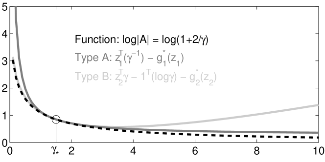
Figure 2: Comparison of type A and B upper bounds on $\log(1+2/\gamma)$.

In general, type A bounding is tighter for $\gamma_{i}$ away from zero, while type B bounding is tighter for $\gamma_{i}$ close to zero (see Figure 2), implications of this point are discussed in Section 5. Whatever bounding type we use, refitting the corresponding upper bound to $\log|\bm{A}|$ requires the computation of $\hat{\bm{z}}=(\mathrm{Var}_{Q}[s_{i}|\bm{y}])$: all marginal variances of the Gaussian distribution $Q(\bm{s}|\bm{y})$. In general, computing Gaussian marginal variances is a hard numerical problem, which is discussed in more detail in Section 4.4.

4.3 The Inner Loop Optimization

The inner loop minimization problem is given by (12), its special case (11) for log-concave potentials and $\log|\bm{A}|$ bounding type A is given by $h_{i}^{*}(s_{i})=-g_{i}(z_{1,i}+s_{i}^{2})$. This problem is of standard penalized least squares form, and a large number of recent algorithms [12, 3, 46] can be applied with little customization efforts. In this section, we provide details about how to apply the iteratively reweighted least squares (IRLS) algorithm [14], a special case of the Newton-Raphson method.

We describe a single IRLS step here, starting from $\bm{u}$. Let $\bm{r}:=\bm{X}\bm{u}-\bm{y}$ denote the residual vector. If $\theta_{i}:=(h_{i}^{*})^{\prime}(s_{i})-b_{i}$, $\rho_{i}:=(h_{i}^{*})^{\prime\prime}(s_{i})$, then

$$\nabla_{\bm{u}}(\phi_{\bm{z}}/2)=\sigma^{-2}\bm{X}^{T}\bm{r}+\bm{B}^{T}\bm{\theta},\quad\nabla\nabla_{\bm{u}}(\phi_{\bm{z}}/2)=\sigma^{-2}\bm{X}^{T}\bm{X}+\bm{B}^{T}(\operatorname{diag}\bm{\rho})\bm{B}.$$

Note that $\rho_{i}\geq 0$ by the convexity of $h_{i}^{*}$. The Newton search direction is

$$\bm{d}:=-(\sigma^{-2}\bm{X}^{T}\bm{X}+\bm{B}^{T}(\operatorname{diag}\bm{\rho})\bm{B})^{-1}(\sigma^{-2}\bm{X}^{T}\bm{r}+\bm{B}^{T}\bm{\theta}).$$

The computation of $\bm{d}$ requires us to solve a system with a matrix of the same form as $\bm{A}$, a reweighted least squares problem otherwise used to compute the means in a Gaussian model of the structure of $Q(\bm{u}|\bm{y})$. We solve these systems approximately by the (preconditioned) linear conjugate gradients (LCG) algorithm [13]. The cost per iteration of LCG is dominated by matrix-vector multiplications (MVMs) with $\bm{X}^{T}\bm{X}$, $\bm{B}$, and $\bm{B}^{T}$. A line search along $\bm{d}$ can be run in negligible time. If $f(t):=\phi_{\bm{z}}(\bm{u}+t\bm{d})/2$, then $f^{\prime}(t)=\sigma^{-2}((\bm{X}\bm{d})^{T}\bm{r}+t\|\bm{X}\bm{d}\|^{2})+(\bm{B}\bm{d})^{T}\bm{\theta}^{(t)}$, where $\bm{\theta}^{(t)}$ is the gradient at $\bm{s}^{(t)}=\bm{s}+t\bm{B}\bm{d}$. With $(\bm{X}\bm{d})^{T}\bm{r}$, $\|\bm{X}\bm{d}\|^{2}$, and $\bm{B}\bm{d}$ precomputed, $f(t)$ and $f^{\prime}(t)$ can be evaluated in $O(q)$ without any further MVMs. The line search is started with $t_{0}=1$. Finally, once $\bm{u}_{*}=\operatorname*{argmin}_{\bm{u}}\phi_{\bm{z}}(\bm{u})$ is found, $\bm{\gamma}$ is explicitly updated as $\operatorname*{argmin}\phi_{\bm{z}}(\bm{u}_{*},\cdot)$. Note that at this point, $\bm{u}_{*}=\mathrm{E}_{Q}[\bm{u}|\bm{y}]$, which follows from the derivation at the beginning of Section 3.

4.4 Estimation of Gaussian Variances

Variational inference does require marginal variances $\hat{\bm{z}}=\operatorname{diag}^{-1}(\bm{B}\bm{A}^{-1}\bm{B}^{T})=(\mathrm{Var}_{Q}[s_{i}|\bm{y}])$ of the Gaussian $Q(\bm{s}|\bm{y})$ (see Section 4.2), which are much harder to approximate than means. In this section, we discuss a general method for (co)variance approximation. Empirically, the performance of our double loop algorithms is remarkably robust in the light of substantial overall variance approximation errors, some insights into this finding are given below.

Marginal posterior variances have to be computed in any approximate Bayesian inference method, while they are not required in typical sparse point estimation techniques (see Section 5). Our double loop algorithms reduce approximate inference to point estimation and Gaussian (co)variance approximation. Not only do they expose the latter as missing link between sparse estimation and variational inference, their main rationale is that Gaussian variances have to be computed a few times only, while off-the-shelf variational optimizers query them for every single criterion evaluation.

Marginal variance approximations have been proposed for sparsely connected Gaussian Markov random fields (MRFs), iterating over embedded spanning tree models [41] or exploiting rapid correlations decay in models with homogeneous prior [20]. In applications of interest here, $\bm{A}$ is neither sparse nor has useful graphical model structure. Committing to a low-rank approximation of the covariance $\bm{A}^{-1}$ [20, 27], an optimal choice in terms of preserving variances is principal components analysis (PCA), based on the smallest eigenvalues/-vectors of $\bm{A}$ (the largest of $\bm{A}^{-1}$). The Lanczos algorithm [13] provides a scalable approximation to PCA and was employed for variance estimation in [27]. After $k$ iterations, we have an orthonormal basis $\bm{Q}_{k}\in\mathbb{R}^{n\times k}$, within which extremal eigenvectors of $\bm{A}$ are rapidly well approximated (due to the nearly linear spectral decay of typical $\bm{A}$ matrices (Figure 6, upper panel), both largest and smallest eigenvalues are obtained). As $\bm{Q}_{k}^{T}\bm{A}\bm{Q}_{k}=\bm{T}_{k}$ is tridiagonal, the Lanczos variance approximation $\hat{\bm{z}}_{k}=\operatorname{diag}^{-1}(\bm{B}\bm{Q}_{k}\bm{T}_{k}^{-1}\bm{Q}_{k}^{T}\bm{B}^{T})$ can be computed efficiently. Importantly, $\hat{z}_{k,i}\leq\hat{z}_{k+1,i}\leq\hat{z}_{i}$ for all $k$ and $i$. Namely, if $\bm{Q}_{k}=[\bm{q}_{1}\dots\bm{q}_{k}]$, and $\bm{T}_{k}$ has main diagonal $(\alpha_{l})$, subdiagonal $(\beta_{l})$, let $(e_{l})$ and $(d_{l})$ be the main and subdiagonal of the bidiagonal Cholesky factor $\bm{L}_{k}$ of $\bm{T}_{k}$. Then, $d_{k-1}=\beta_{k-1}/e_{k-1}$, $e_{k}=(\alpha_{k}-d_{k-1}^{2})^{1/2}$, with $d_{0}=0$. If $\bm{V}_{k}:=\bm{B}\bm{Q}_{k}\bm{L}_{k}^{-T}$, we have $\bm{V}_{k}=[\bm{v}_{1}\dots\bm{v}_{k}]$, $\bm{v}_{k}=(\bm{B}\bm{q}_{k}-d_{k-1}\bm{v}_{k-1})/e_{k}$. Finally, $\hat{\bm{z}}_{k}=\hat{\bm{z}}_{k-1}+\bm{v}_{k}^{2}$ (with $\hat{\bm{z}}_{0}=\bm{0}$).

Unfortunately, the Lanczos algorithm is much harder to run in practice than LCG, and its cost grows superlinearly in $k$. A promising variant of selectively reorthogonalized Lanczos [24] is given in [2], where contributions from undesired parts of the spectrum ($\bm{A}$’s largest eigenvalues in our case) are filtered out by replacing $\bm{A}$ with polynomials of itself. Recently, randomized PCA approaches have become popular [15], although their relevance for variance approximation is unclear. Nevertheless, for large scale problems of interest, standard Lanczos can be run for $k\ll n$ iterations only, at which point most of the $\hat{z}_{k,i}$ are severely underestimated (see Section 7.3). Since Gaussian variances are essential for variational Bayesian inference, yet scalable, uniformly accurate variance estimators are not known, robustness to variance approximations errors is critical for any large scale approximate inference algorithm.

What do the Lanczos variance approximation errors imply for our double loop algorithms? First, the global convergence proof of Section 4.1 requires exact variances $\hat{\bm{z}}$, thus may be compromised if $\hat{\bm{z}}_{k}$ is used instead. This problem is analyzed in [31]: the convergence proof remains valid with the PCA approximation, which however is different from the Lanczos approximation. Empirically, we did not encounter convergence problems so far.

Surprisingly, while $\hat{\bm{z}}_{k}$ is much smaller than $\hat{\bm{z}}$ in practice, there is little indication of substantial negative impact on performance. This important robustness property is analyzed in Section 7.3 for an SLM with Laplace potentials. The underestimation bias has systematic structure (Figure 6, middle and lower panel): moderately small $\hat{z}_{i}$ are damped most strongly, while large $\hat{z}_{i}$ are approximated accurately. This happens because the largest coefficients $\hat{z}_{i}$ depend most strongly on the largest covariance eigenvectors, which are shaped in early Lanczos iterations. This particular error structure has statistical consequences. Recalling the inner loop penalty for Laplacians (2): $h_{i}^{*}(s_{i})=\tau_{i}(\hat{z}_{i}+s_{i}^{2})^{1/2}$, the smaller $\hat{z}_{i}$, the stronger it enforces sparsity. If $\hat{z}_{i}$ is underestimated, the penalty on $s_{i}$ is stronger than intended, yet this strengthening does not happen uniformly. Coefficients $s_{i}$ deemed most relevant with exact variance computation (largest $\hat{z}_{i}$) are least affected (as $\hat{z}_{k,i}\approx\hat{z}_{i}$ for those), while already subdominant ones (smaller $\hat{z}_{i}$) are suppressed even stronger (as $\hat{z}_{k,i}\ll\hat{z}_{i}$). At least in our experience so far (with sparse linear models), this selective variance underestimation effect seems benign or even somewhat beneficial.

4.5 Extension to Group Potentials

There is substantial recent interest in methods incorporating sparse group penalization, meaning that a number of latent coefficients (such as the column of a matrix, or the incoming edge weights for a graph) are penalized jointly [47, 40]. Our algorithms are easily generalized to models with potentials of the form $t_{i}(\|\bm{s}_{i}\|)$, $\bm{s}_{i}$ a subvector of $\bm{s}$, $\|\cdot\|$ the Euclidean norm, if $t_{i}(\cdot)$ is even and super-Gaussian. Such group potentials are frequently used in practice. The isotropic total variation penalty is the sum of $\|(dx_{i},dy_{i})\|$, $dx_{i}$, $dy_{i}$ differences along different axes, which corresponds to group Laplace potentials. In our MRI application (Section 7.4), we deal with complex-valued $\bm{u}$ and $\bm{s}$. Each entry is treated as element in $\mathbb{R}^{2}$, and potentials are placed on $|s_{i}|=\|(\Re s_{i},\Im s_{i})\|$. Note that with $t_{i}$ on $\|\bm{s}_{i}\|$, the single parameter $\gamma_{i}$ is shared by the coefficients $\bm{s}_{i}$.

The generalization of our algorithms to group potentials is almost automatic. For example, if all $\bm{s}_{i}$ have the same dimensionality, $\bm{\Gamma}^{-1}$ is replaced by $\bm{\Gamma}^{-1}\otimes\bm{I}$ in the definition of $\bm{A}$, and $\hat{\bm{z}}$ is replaced by $(\bm{I}\otimes\bm{1}{}^{T})\operatorname{diag}^{-1}(\bm{B}\bm{A}^{-1}\bm{B}^{T})$ in Section 4.2. Moreover, $x_{i}=s_{i}^{2}$ is replaced by $x_{i}=\|\bm{s}_{i}\|^{2}$, whereas the definition of $g_{i}(x_{i})$ remains the same. Apart from these simple replacements, only IRLS inner loop iterations have to be modified (at no extra cost), as is detailed in Appendix A.7.

4.6 Publicly Available Code: The glm-ie Toolbox

Algorithms and techniques presented in this paper are implemented as part of the generalized linear model inference and estimation toolbox (glm-ie), maintained as mloss.org project at mloss.org/software/view/269/. The code runs with both Matlab 7 and the free Octave 3.2. It comprises algorithms for MAP (penalized least squares) estimation and variational inference in generalized linear models (Section 4), along with Lanczos code for Gaussian variances (Section 4.4).

Its generic design allows for a range of applications, as illustrated by a number of example programs included in the package. Many super-Gaussian potentials $t_{i}(s_{i})$ are included, others can easily be added by the user. In particular, the toolbox contains a range of solvers for MAP and inner loop problems, from IRLS (or truncated Newton, see Section 4.3) over conjugate gradients to Quasi-Newton, as well as a range of commonly used operators to construct $\bm{X}$ and $\bm{B}$ matrices.

5 Sparse Estimation and Sparse Bayesian Inference

In this section, we contrast approximate Bayesian inference with point estimation for sparse linear models (SLMs): sparse Bayesian inference versus sparse estimation. These problem classes serve distinct goals and come with different algorithmic characteristics, yet are frequently confused in the literature. Briefly, the goal in sparse estimation is to eliminate variables not needed for the task at hand, while sparse inference aims at quantifying uncertainty in decisions and dependencies between components. While variable elimination is a boon for efficient computation, it cannot be relied upon in sparse inference. Sensible uncertainty estimates like posterior covariance, at the heart of decision-making problems such as Bayesian experimental design, are eliminated alongside.

We restrict ourselves to super-Gaussian SLM problems in terms of variables $\bm{u}$ and $\bm{\gamma}\succeq\bm{0}$, relating the sparse Bayesian inference relaxation $\min_{\bm{\gamma}\succeq\bm{0}}\phi(\bm{\gamma})$ with two sparse estimation principles: maximum a posteriori (MAP) reconstruction (10) and automatic relevance determination (ARD) [43], a sparse reconstruction method which inspired our algorithms. We begin by establishing a key difference between these settings. Recall from Theorem 1(4) that $\gamma_{i}=0$ implies $\mathrm{Var}_{Q}[s_{i}|\bm{y}]=0$: $s_{i}$ is eliminated, fixed at zero with absolute certainty. Exact sparsity in $\bm{\gamma}$ does not happen for inference, while sparse estimation methods are characterized by fixing many $\gamma_{i}$ to zero.

Theorem 4

Let $\bm{X}\in\mathbb{R}^{m\times n}$, $\bm{B}\in\mathbb{R}^{q\times n}$ be matrices such that $\tilde{\bm{A}}(\bm{\pi})=\sigma^{-2}\bm{X}^{T}\bm{X}+\bm{B}^{T}(\operatorname{diag}\bm{\pi})\bm{B}\succ\bm{0}$ for each $\bm{\pi}\succ\bm{0}$, and no row of $\bm{B}$ is equal to $\bm{0}^{T}$.

• The function $\log|\tilde{\bm{A}}(\bm{\pi})|$ is increasing in each component $\pi_{i}$, and unbounded above. For any sequence $\bm{\pi}_{t}$ with $\|\bm{\pi}_{t}\|\to\infty$ ($t\to\infty$) and $\bm{\pi}_{t}\succeq\mathrm{\varepsilon}\bm{1}$ for some $\mathrm{\varepsilon}>0$, we have that $\log|\tilde{\bm{A}}(\bm{\pi}_{t})|\to\infty$ ($t\to\infty$).

• Assume that $\log P(\bm{u}|\bm{y})$ is bounded above as function of $\bm{u}$. Recall the variational criterion $\phi(\bm{\gamma})$ from (9). For any bounded sequence $\bm{\gamma}_{t}$ with $(\bm{\gamma}_{t})_{i}\to 0$ ($t\to\infty$) for some $i\in\{{1},\dots,{q}\}$, we have that $\phi(\bm{\gamma}_{t})\to\infty$.
  In particular, any local minimum point $\bm{\gamma}_{*}$ of the variational inference problem $\min_{\bm{\gamma}\succeq\bm{0}}\phi(\bm{\gamma})$ must have positive components: $\bm{\gamma}_{*}\succ\bm{0}$.

A proof is given in Appendix A.3. $\log|\bm{A}|$ acts as barrier function for $\bm{\gamma}\succ\bm{0}$. Any local minimum point $\bm{\gamma}_{*}$ of (9) is positive throughout, and $\mathrm{Var}_{Q}[s_{i}|\bm{y}]>0$ for all $i={1},\dots,{q}$. Coefficient elimination does not happen in variational Bayesian inference.

Consider MAP estimation (10) with even super-Gaussian potentials $t_{i}(s_{i})$. Following [25], a sufficient condition for sparsity is that $-\log t_{i}(s_{i})$ is concave for $s_{i}>0$. In this case, if $\operatorname{rk}\bm{X}=m$ and $\operatorname{rk}\bm{B}=n$, then any local MAP solution $\bm{u}_{*}$ is exactly sparse: no more than $m$ coefficients of $\bm{s}_{*}=\bm{B}\bm{u}_{*}$ are nonzero. Examples are $t_{i}(s_{i})=e^{-\tau_{i}|s_{i}|^{p}}$, $p\in(0,1]$, including Laplace potentials ($p=1$). Moreover, $\gamma_{*.i}=0$ whenever $s_{*,i}=0$ in this case (see Appendix A.3). Local minimum points of SLM MAP estimation are substantially exactly sparse, with matching sparsity patterns of $\bm{s}_{*}=\bm{B}\bm{u}_{*}$ and $\bm{\gamma}_{*}$.

A powerful sparse estimation method, automatic relevance determination (ARD) [43], has inspired our approximate inference algorithms developed above. The ARD criterion $\phi_{\text{ARD}}$ is (9) with $h(\bm{\gamma})=\bm{1}^{T}(\log\bm{\gamma})$, obtained as zero-temperature limit ($\nu\to 0$) of variational inference with Student’s t potentials (3). The function $h_{i}(\gamma_{i})$ is given in Appendix A.6, and $h_{i}(\gamma_{i})\to\log\gamma_{i}$ ($\nu\to 0$) if additive constants independent of $\gamma_{i}$ are dropped. ARD can also be seen as marginal likelihood maximization: $\phi_{\text{ARD}}(\bm{\gamma})=-2\log\int P(\bm{y}|\bm{u})N(\bm{s}|\bm{0},\bm{\Gamma})\,d\bm{u}$ up to an additive constant. Sparsity penalization is implied by the fact that the prior $N(\bm{s}|\bm{0},\bm{\Gamma})$ is normalized (see Figure 3, left). The ARD problem is not convex. A provably convergent double loop ARD algorithm is obtained by employing bounding type B (Section 4.2), along similar lines to Section 4.1 we obtain

$$\min_{\bm{\gamma}\succeq\bm{0}}\phi_{\text{ARD}}(\bm{\gamma})=\min_{\bm{z}_{2}\succeq\bm{0}}\left(\min_{\bm{u}}\sigma^{-2}\|\bm{y}-\bm{X}\bm{u}\|^{2}+2\sum\nolimits_{i=1}^{q}z_{2,i}^{1/2}|s_{i}|\right)-g_{2}^{*}(\bm{z}_{2}).$$

The inner problem is $\ell_{1}$ penalized least squares estimation, a reweighted variant of MAP reconstruction for Laplace potentials. Its solutions $\bm{s}_{*}=\bm{B}\bm{u}_{*}$ are exactly sparse, along with corresponding $\bm{\gamma}_{*}$ (since $\gamma_{*,i}=z_{2,i}^{-1/2}|s_{*,i}|$). ARD is enforcing sparsity more aggressively than Laplace ($\ell_{1}$) MAP reconstruction [44]. The $\log|\bm{A}|$ barrier function is counterbalanced by $h(\bm{\gamma})=\bm{1}^{T}(\log\bm{\gamma})=\log|\bm{\Gamma}|$. If $\bm{B}=\bm{I}$, then

$$\log|\bm{A}|+\log|\bm{\Gamma}|=\log|\bm{I}+\sigma^{-2}\bm{X}\bm{\Gamma}\bm{X}^{T}|\to 0\;(\bm{\gamma}\to\bm{0}).$$

The conceptual difference between ARD and our variational inference relaxation is illustrated in Figure 3. In sparse inference, Gaussian functions $e^{-s_{i}^{2}/(2\gamma_{i})-h_{i}(\gamma_{i})/2}$ lower bound $t_{i}(s_{i})$. Their mass vanishes as $\gamma_{i}\to 0$, driving $\phi(\bm{\gamma})\to\infty$. For ARD, Gaussian functions $N(s_{i}|0,\gamma_{i})$ are normalized, and $\gamma_{i}\to 0$ is encouraged.

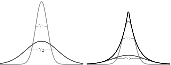
Figure 3: Different roles of Gaussian functions (width $\gamma_{i}$) in sparse estimation versus sparse inference. Left: Sparse estimation (ARD). Gaussian functions are normalized, there is incentive to drive $\gamma_{i}\to 0$. Right: Variational inference for Laplace potentials (2). Gaussian functions are lower bounds of $t_{i}(s_{i})$, their mass vanishes as $\gamma_{i}\to 0$. No incentive to eliminate $\gamma_{i}$.

At this point, the roles of different bounding types introduced in Section 4.2 become transparent. $\log|\bm{A}|$ is a barrier function for $\bm{\gamma}\succ\bm{0}$ (Theorem 4), as is its type A bound $\bm{z}_{1}^{T}(\bm{\gamma}^{-1})-g_{1}^{*}(\bm{z}_{1})$, $\bm{z}_{1}\succ\bm{0}$ (see Figure 2). On the other hand, $\log|\bm{A}|+\bm{1}^{T}(\log\bm{\gamma})$ is bounded below, as is its type B bound $\bm{z}_{2}^{T}\bm{\gamma}-g_{2}^{*}(\bm{z}_{2})$. These facts suggest that type A bounding should be preferred for variational inference, while type B bounding is best suited for sparse estimation. Indeed, experiments in Section 7.1 show that for approximate inference with Laplace potentials, type A bounding is by far the better choice, while for ARD, type B bounding leads to the very efficient algorithm just sketched.

Sparse estimation methods eliminate a substantial fraction of $\bm{\gamma}$’s coefficients, variational inference methods do not zero any of them. This difference has important computational and statistical implications. First, exact sparsity in $\bm{\gamma}$ is computationally beneficial. In this regime, even coordinate descent algorithms can be scaled up to large problems [39]. Within the ARD sparse estimation algorithm, variances $\hat{\bm{z}}\leftarrow\operatorname{diag}^{-1}(\bm{B}\bm{A}^{-1}\bm{B}^{T})$ have to be computed, but since $\hat{\bm{z}}$ is as sparse as $\bm{\gamma}$, this is not a hard problem. Variational inference methods have to cope without exact sparsity. The double loop algorithms of Section 4 are scalable nevertheless, reducing to numerical techniques whose performance does not depend on the sparsity of $\bm{\gamma}$.

While exact sparsity in $\bm{\gamma}$ implies computational simplifications, it also rules out proper model-based uncertainty quantification. If $\gamma_{i}=0$, then $\mathrm{Var}_{Q}[s_{i}|\bm{y}]=0$. If $Q(\bm{u}|\bm{y})$ is understood as representation of uncertainty, it asserts that there is no posterior variance in $s_{i}$ at all: $s_{i}$ is eliminated with absolute certainty, along with all correlations between $s_{i}$ and other $s_{j}$. Sparsity in $\bm{\gamma}$ is computationally useful only if most $\gamma_{i}=0$. $Q(\bm{u}|\bm{y})$, a degenerate distribution with mass only in the subspace corresponding to surviving coefficients, cannot sensibly be regarded as approximation to a Bayesian posterior. As zero is just zero, even basic queries such as a confidence ranking over eliminated coefficients cannot be based on a degenerate $Q(\bm{u}|\bm{y})$.

In particular, Bayesian experimental design (Section 6) cannot sensibly be driven by underlying sparse estimation technology, while it excels for a range of real-world scenarios (see Section 7.4) when based on a sparse inference method [36, 28, 32, 34]. The former approach is taken in [18], employing the sparse Bayesian learning estimator [38] to drive inference queries. Their approach fails badly on real-world image data [32]. Started with few initial measurements, it identifies a very small subspace of non-eliminated coefficients (as expected for sparse estimation fed with little data), which it essentially remains locked in ever after. To sensibly score a candidate $\bm{X}_{*}$, we have to reason about what happens to all coefficients, which is not possible based on a “posterior” $Q(\bm{u}|\bm{y})$ ruling out most of them with full certainty.

Finally, even if the goal is point reconstruction from given data, the sparse inference posterior mean $\mathrm{E}_{Q}[\bm{u}|\bm{y}]$ (obtained as byproduct $\bm{u}_{*}$ in the double loop algorithm of Section 4) can be an important alternative to an exactly sparse estimator. For the former, $\mathrm{E}_{Q}[\bm{s}|\bm{y}]=\bm{B}\bm{u}_{*}$ is not sparse in general, and the degree to which coefficients are penalized (but not eliminated) is determined by the choice of $t_{i}(s_{i})$. To illustrate this point, we compare the mean estimator for Laplace and Student’s t potentials (different $\nu>2$) in Section 7.2. These results demonstrate that contrary to some folklore in signal and image processing, sparser is not necessarily better for point reconstruction of real-world images. Enforcing sparsity too strongly leads to fine details being smoothed out, which is not acceptable in medical imaging (fine features are often diagnostically most relevant) or photography postprocessing (most users strongly dislike unnaturally hard edges and oversmoothed areas).

Sparse estimation methodology has seen impressive advancements towards what it is intended to do: solving a given overparameterized reconstruction problem by eliminating nonessential variables. However, it is ill-suited for addressing decision-making scenarios driven by Bayesian inference. For the latter, a useful (nondegenerate) posterior approximation has to be obtained without relying on computational benefits of exact sparsity. We show how this can be done, by reducing variational inference to numerical techniques (LCG and Lanczos) which can be scaled up to large problems without exact variable sparsity.

6 Bayesian Experimental Design

In this section, we show how to optimize the image acquisition matrix $\bm{X}$ by way of Bayesian sequential experimental design (also known as Bayesian active learning), maximizing the expected amount of information gained. Unrelated to the output of point reconstruction methods, information gain scores depend on the posterior covariance matrix $\mathrm{Cov}[\bm{u}|\bm{y}]$ over full images $\bm{u}$, which within our large scale variational inference framework is approximated by the Lanczos algorithm.

In each round, a part $\bm{X}_{*}\in\mathbb{R}^{d\times n}$ is appended to the design $\bm{X}$, a new (partial) measurement $\bm{y}_{*}$ to $\bm{y}$. Candidates $\{\bm{X}_{*}\}$ are ranked by the information gain score $\mathrm{H}[P(\bm{u}|\bm{y})]-\mathrm{E}_{P(\bm{y}_{*}|\bm{y})}[\mathrm{H}[P(\bm{u}|\bm{y},\bm{y}_{*})]]$, where $P(\bm{u}|\bm{y})$ and $P(\bm{u}|\bm{y},\bm{y}_{*})$ are posteriors for $(\bm{X},\bm{y})$ and $(\bm{X}\cup\bm{X}_{*},\bm{y}\cup\bm{y}_{*})$ respectively, and $P(\bm{y}_{*}|\bm{y})=\int N(\bm{y}_{*}|\bm{X}_{*}\bm{u},\sigma^{2}\bm{I})P(\bm{u}|\bm{y})\,d\bm{u}$. Replacing $P(\bm{u}|\bm{y})$ by its best Gaussian variational approximation $Q(\bm{u}|\bm{y})=N(\bm{u}_{*},\bm{A}^{-1})$ and $P(\bm{u}|\bm{y},\bm{y}_{*})$ by $Q(\bm{u}|\bm{y},\bm{y}_{*})\propto N(\bm{y}_{*}|\bm{X}_{*}\bm{u},\sigma^{2}\bm{I})Q(\bm{u}|\bm{y})$, we obtain an approximate information gain score

$$\Delta(\bm{X}_{*}):=-\log|\bm{A}|+\log\left|\bm{A}+\sigma^{-2}\bm{X}_{*}^{T}\bm{X}_{*}\right|=\log\left|\bm{I}+\sigma^{-2}\bm{X}_{*}\bm{A}^{-1}\bm{X}_{*}^{T}\right|.$$ (13)

Note that $Q(\bm{u}|\bm{y},\bm{y}_{*})$ has the same variational parameters $\bm{\gamma}$ as $Q(\bm{u}|\bm{y})$, which simplifies and robustifies score computations. Refitting of $\bm{\gamma}$ is done at the end of each round, once the score maximizer $\bm{X}_{*}$ is appended along with a new measurement $\bm{y}_{*}$.

With $N$ candidates of size $d$ to be scored, a naive computation of (13) would require $N\cdot d$ linear systems to be solved, which is not tractable (for example, $N=240$, $d=512$ in Section 7.4). We can make use of the Lanczos approximation once more (see Section 4.4). If $\bm{Q}_{k}^{T}\bm{A}\bm{Q}_{k}=\bm{T}_{k}=\bm{L}_{k}\bm{L}_{k}^{T}$ ($\bm{L}_{k}$ is bidiagonal, computed in $O(k)$), let $\bm{V}_{*}:=\sigma^{-1}\bm{X}_{*}\bm{Q}_{k}\bm{L}_{k}^{-T}\in\mathbb{R}^{d\times k}$. Then, $\Delta(\bm{X}_{*})\approx\log|\bm{I}+\bm{V}_{*}\bm{V}_{*}^{T}|=\log|\bm{I}+\bm{V}_{*}^{T}\bm{V}_{*}|$ (the latter is preferable if $k<d$), at a total cost of $k$ matrix-vector multiplications (MVMs) with $\bm{X}_{*}$ and $O(\max\{k,d\}\cdot\min\{k,d\}^{2})$. Just as with marginal variances, Lanczos approximations of $\Delta(\bm{X}_{*})$ are underestimates, nondecreasing in $k$. The impact of Lanczos approximation errors on design decisions is analyzed in [31]. While absolute score values are much too small, decisions only depend on the ranking among the highest-scoring candidates $\bm{X}_{*}$, which often is faithfully reproduced even for $k\ll n$. To understand this point, note that $\Delta(\bm{X}_{*})$ measures the alignment of $\bm{X}_{*}$ with the directions of largest variance in $Q(\bm{u}|\bm{y})$. For example, the single best unit-norm filter $\bm{x}_{*}\in\mathbb{R}^{n}$ is given by the maximal eigenvector of $\mathrm{Cov}_{Q}[\bm{u}|\bm{y}]=\bm{A}^{-1}$, which is obtained after few Lanczos iterations.

In the context of Bayesian experimental design, the convexity of our variational inference relaxation (with log-concave potentials) is an important asset. In contrast to single image reconstruction, which can be tuned by the user until a desired result is obtained, sequential acquisition optimization is an autonomous process consisting of many individual steps (a real-world example is given in Section 7.4), each of which requires a variational refitting $Q(\bm{u}|\bm{y})\to Q(\bm{u}|\bm{y},\bm{y}_{*})$. Within our framework, each of these has a unique solution which is found by a very efficient algorithm. While we are not aware of Bayesian acquisition optimization being realized at comparable scales with other inference approximations, this would be difficult to do indeed. Different variational approximations are non-convex problems coming with notorious local minima issues. For Markov chain Monte Carlo methods, there are not even reliable automatic tests of convergence. If approximate inference drives a multi-step automated scheme free of human expert interventions, properties like convexity and robustness gain relevance normally overlooked in the literature.

6.1 Compressive Sensing of Natural Images

The main application we address in Section 7.4, automatic acquisition optimization for magnetic resonance imaging, is an advanced real-world instance of compressive sensing (CS) [6, 5]. Given that real-world images come with low entropy super-Gaussian statistics, how can we tractably reconstruct them from a sample below the Nyquist-Shannon limit? How do small successful designs $\bm{X}$ for natural images look like? Recent celebrated results about recovery properties of convex sparse estimators [10, 6, 5] have been interpreted as suggesting that up from a certain size, successful designs $\bm{X}$ may simply be drawn blindly at random. Technically speaking, these results are about highly exactly sparse signals (see Section 5), yet advancements for image reconstruction are typically being implied [6, 5]. In contrast, Bayesian experimental design is an adaptive approach, optimizing $\bm{X}$ based on real-world training images. Our work is of the latter kind, as are [18, 32, 16] for much smaller scales.

The question whether a design $\bm{X}$ is useful for measuring images, can (and should) be resolved empirically. Indeed, it takes not more than some reconstruction code and a range of realistic images (natural photographs, MR images) to convince oneself that MAP estimation from a subset of Fourier coefficients drawn uniformly at random (say, at $1/4$ Nyquist) leads to very poor results. This failure of blindly drawn designs is well established by now both for natural images and MR images [32, 34, 19, 7], and is not hard to motivate. In a nutshell, the assumptions which current CS theory relies upon do not sensibly describe realistic images. Marginal statistics of the latter are not exactly sparse, but exhibit a power law (super-Gaussian) decay. More important, their sparsity is highly structured, a fact which is ignored in assumptions made by current CS theory, therefore not reflected in recovery conditions (such as incoherence) or in designs $\bm{X}$ drawn uniformly at random. Such designs fail for a number of reasons. First, they do not sample where the image energy is [32, 7]. A more subtle problem is the inherent variability of independent sampling in Fourier space: large gaps occur with high probability, which leads to serious MAP reconstruction errors. These points are reinforced in [32, 34]. The former study finds that for good reconstruction quality of real-world images, the choice of $\bm{X}$ is far more important than the type of reconstruction algorithm used.

In real-world imaging applications, adaptive approaches promise remedies for these problems (other proposals in this direction are [18] and [16], which however have not successfully been applied to real-world images). Instead of relying on simplistic signal assumptions, they learn a design $\bm{X}$ from realistic image data. Bayesian experimental design provides a general framework for adaptive design optimization, driven not by point reconstruction, but by predicting information gain through posterior covariance estimates.

7 Experiments

We begin with a set of experiments designed to explore aspects and variants of our algorithms, and to understand approximation errors. Our main application concerns the optimization of sampling trajectories in magnetic resonance imaging (MRI) sequences, with the aim of obtaining useful images faster than previously possible.

7.1 Type A versus Type B Bounding for Laplace Potentials

Recall that the critical coupling term $\log|\bm{A}|$ in the variational criterion $\phi(\bm{\gamma})$ can be upper bounded in two different ways, called type A and type B in Section 4.2. Type A is tight for moderate and large $\gamma_{i}$, type B for small $\gamma_{i}$ (Section 5). In this section, we run our inference algorithm with type A and type B bounding respectively, comparing the speed of convergence. The setup (SLM with Laplace potentials) is as detailed in Section 7.4, with a design $\bm{X}$ of 64 phase encodes ($1/4$ Nyquist). Results are given in Figure 4, averaged over 7 different slices from sg88 ($256\times 256$ pixels, $n=131072$).

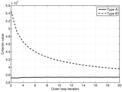
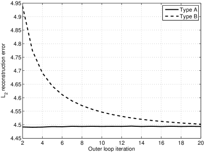
Figure 4: Comparison of bounding types A, B for SLM with Laplace potentials. Shown are $\phi(\bm{\gamma})$ criterion values (left) and $\ell_{2}$ errors of posterior mean estimates (not MAP, as in Section 7.4), at the end of each outer loop iteration (starting from second).

In this case, the bounding type strongly influences the algorithm’s progress. While two outer loop (OL) iterations suffice for convergence with type A, convergence is not attained even after 20 OL steps with type B. More inner loop (IL) steps are done for type A (30 in first OL iteration, 3–4 afterwards) than for type B (5–6 in first OL iteration, 3–4 afterwards). The double loop strategy, to make substantial progress with far less expensive IL updates, works out for type A, but not for type B bounding. These results indicate that bounding type A should be preferred for SLM variational inference, certainly with Laplace potentials. Another indication comes from comparing IL penalties $h_{i}^{*}(s_{i})$ respectively. For type A, $h_{i}^{*}(s_{i})=\tau_{i}(z_{1,i}+s_{i}^{2})^{1/2}$ is sparsity-enforcing for small $z_{1,i}$, retaining an important property of $\phi(\bm{\gamma})$, while for type B, $h_{i}^{*}(s_{i})$ does not enforce sparsity at all (see Appendix A.6).

7.2 Student’s t Potentials

In this section, we compare SLM variational inference with Student’s t (3) potentials to the Laplace setup of Section 7.1. Student’s t potentials are not log-concave, so neither MAP estimation nor variational inference are convex problems. Student’s t potentials enforce sparsity more strongly than Laplacians do, which is often claimed to be more useful for image reconstruction. Their parameters are $\nu$ (degrees of freedom; regulating sparsity) and $\alpha=\nu/\tau$ (scale). We compare Laplace and Student’s t potentials of same variance (the latter has a variance for $\nu>2$ only): $\alpha_{a}=2(\nu-2)/\tau_{a}^{2}$, where $\tau_{a}$ is the Laplace parameter, $\alpha_{r}$, $\alpha_{i}$ respectively. The model setup is the same as in Section 7.1, using slice 8 of sg88 only. Result are given in Figure 5.

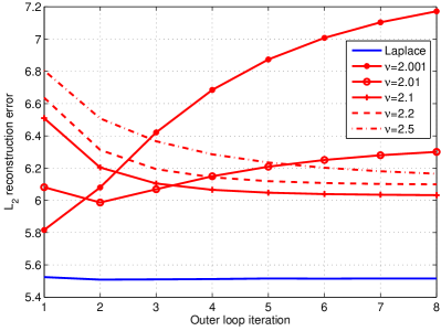
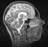
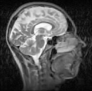
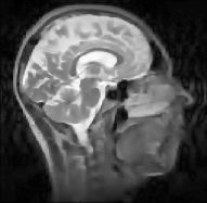
Figure 5: Comparison of SLM with Student’s t and Laplace potentials (type A bounding). Shown are potential density functions (upper left), $\ell_{2}$ errors of posterior mean estimates (upper right), over 8 outer loop iterations. Lower row: Posterior mean reconstructions $(|u_{*,i}|)$ after 8 OL iterations: $\nu=2.1$; ground truth; $\nu=2.01$; $\nu=2.001$.

Compared to the Laplace setup, reconstruction errors for Student’s t SLMs are worse across all values of $\nu$. While $\nu=2.1$ outperforms larger values, the reconstruction error grows with iterations for $\nu=2.01$, $\nu=2.001$. This is not a problem of sluggish convergence: $\phi(\bm{\gamma})$ decreases rapidly in this case. A glance at the mean reconstructions $(|u_{*,i}|)$ (Figure 5, lower row) indicates what happens. For $\nu=2.01,2.001$, image sparsity is clearly enforced too strongly, leading to fine features being smoothed out. The reconstruction for $\nu=2.001$ is merely a caricature of the real image complexity, and rather useless as the output of a medical imaging procedure. When it comes to real-world image reconstruction, more sparsity does not necessarily lead to better results.

7.3 Inaccurate Lanczos Variance Estimates

The difficulty of large scale Gaussian variance approximation is discussed in Section 4.4. In this section, we analyse errors of the Lanczos variance approximation we employ in our experiments. We downsampled our MRI data to $64\times 64$, to allow for ground truth exact variance computations. The setup is the same as above (Laplacians, type A bounding), with $\bm{X}$ consisting of 30 phase encodes. Starting with a single common OL iteration, we compare different ways of updating $\bm{z}_{1}$: exact variance computations versus Lanczos approximations of different size $k$. Results are given in Figure 6 (upper and middle row).

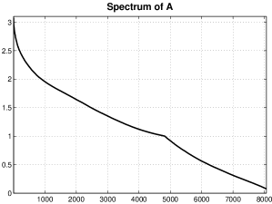
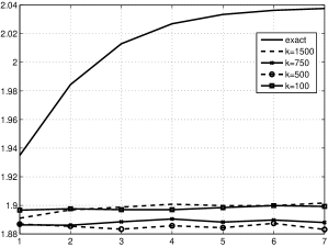
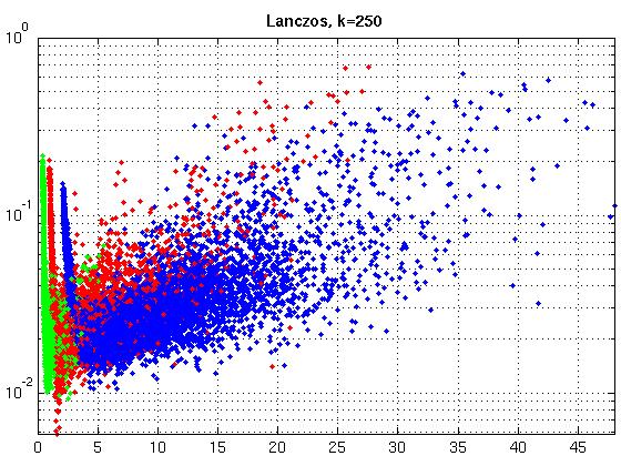
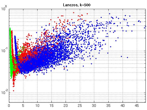
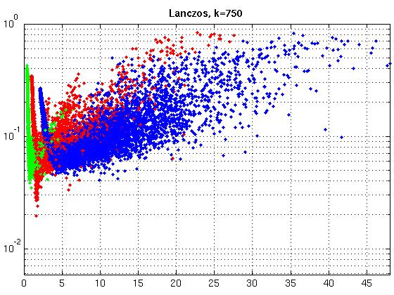
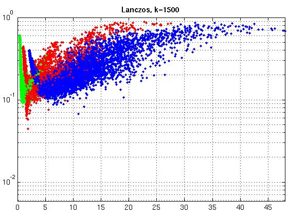
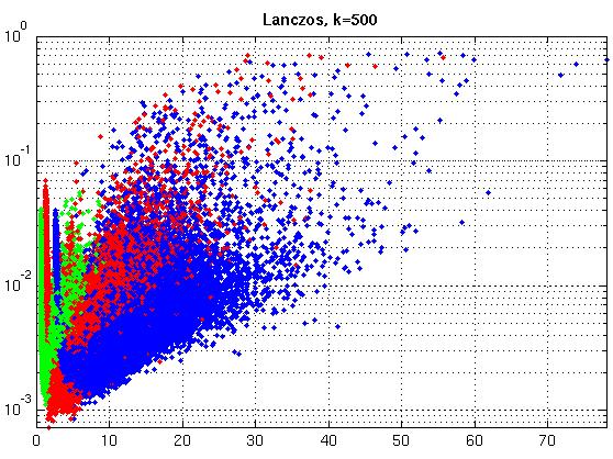
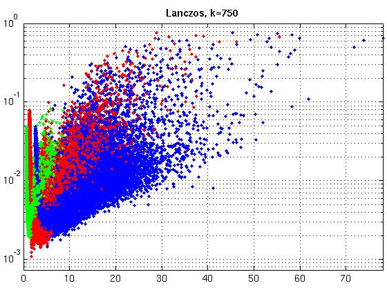
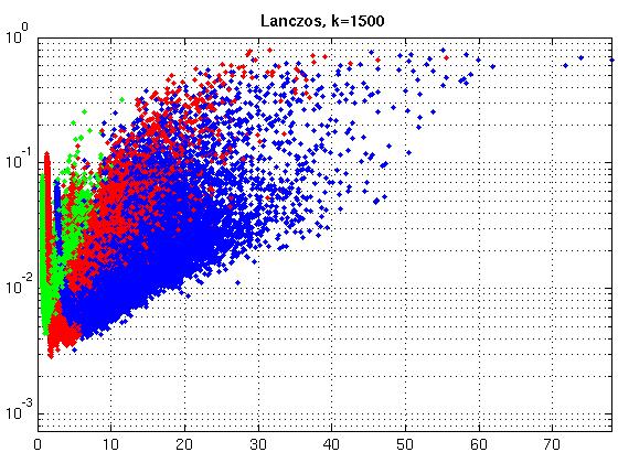
Figure 6: Lanczos approximations of Gaussian variances, at beginning of second OL iteration. For $64\times 64$ data (upper left), spectral decay of inverse covariance matrix $\bm{A}$ is roughly linear (upper middle). $\ell_{2}$ reconstruction error of posterior mean estimate after subsequent OL iterations, for exact variance computation vs. $k=250,500,750,1500$ Lanczos steps (upper right). Middle row: Relative accuracy $\hat{z}_{i}\mapsto\hat{z}_{k,i}/\hat{z}_{i}$ at beginning of second OL iteration, separately for “a” potentials (on wavelet coefficients; red), “r” potentials (on derivatives; blue), and “i” potentials (on $\Im(\bm{u})$; green), see Section 7.4. Lower row: Relative accuracy $\hat{z}_{i}\mapsto\hat{z}_{k,i}/\hat{z}_{i}$ at beginning of second OL iteration, for full size setup ($256\times 256$), $k=500,750,1500$ (ground truth $\hat{z}_{i}$ determined by separate LCG runs).

The spectrum of $\bm{A}$ at the beginning of the second OL iteration shows a roughly linear decay. Lanczos approximation errors are rather large (middle row). Interestingly, the algorithm does certainly not work better with exact variance computations (judged by the development of posterior mean reconstruction errors, upper right). We offer a heuristical explanation in Section 4.4. A clear structure in the relative errors emerges from the middle row: the largest (and also smallest) true values $\hat{z}_{i}$ are approximated rather accurately, while smaller true entries are strongly damped. The role of sparsity potentials $t_{i}(s_{i})$, or of $\gamma_{i}$ within the variational approximation, is to shrink coefficients selectively. The structure of Lanczos variance errors serves to strengthen this effect. We repeated the relative error estimation for the full-scale setup used in the previous sections and below ($256\times 256$), ground truth values $\hat{z}_{i}$ were obtained by separate conjugate gradients runs. The results (shown in the lower row) exhibit the same structure, although relative errors are larger in general.

Both our experiments and our heuristic explanation are given for sparse linear model inference, we do not expect them to generalize to other models. Within the same model and problem class, the impact of Lanczos approximations on final design outcomes is analyzed in [31]. As noted in Section 4.4, understanding the real impact of Lanczos (or PCA) approximations on approximate inference and decision-making is an important topic for future research.

7.4 Sampling Optimization for Magnetic Resonance Imaging

Magnetic resonance imaging [45] is among the most important medical imaging modalities. Without applying any harmful ionizing radiation, a wide range of parameters, from basic anatomy to blood flow, brain function or metabolite distribution, can be visualized. Image slices are reconstructed from coefficients sampled along smooth trajectories in Fourier space (phase encodes). In Cartesian MRI, phase encodes are dense columns or rows in discrete Fourier space. The most serious limiting factor is long scan time, which is proportional to the number of phase encodes acquired. MRI is a prime candidate for compressive sensing (Section 6.1) in practice [19, 34]: if images of diagnostic quality can be reconstructed from an undersampled design, time is saved at no additional hardware costs or risks to patients.

In this section, we address the problem of MRI sampling optimization: which smallest subset of phase encodes results in MAP reconstructions of useful quality? To be clear, we do not use approximate Bayesian technology to improve reconstruction from fixed designs (see Section 5), but aim to optimize the design $\bm{X}$ itself, so to best support subsequent standard MAP reconstruction on real-world images. As discussed in Section 5 and Section 6.1, the focus for most work on compressive sensing is on the reconstruction algorithm, the question of how to choose $\bm{X}$ is typically not addressed (exceptions include [18, 16]). We follow the adaptive Bayesian experimental design scenario described in Section 6, where $\{\bm{X}_{*}\}$ are phase encodes (columns in Fourier space), $\bm{u}$ the unknown (complex-valued) image. Implementing this proposal requires the approximation of dominating posterior covariance directions for a large scale non-Gaussian SLM ($n=131072$), which to our knowledge has not been attempted before. Results shown below are part of a larger study [34] on human brain data acquired with a Siemens 3T scanner (TSE, 23 echos$/$exc, $120^{\circ}$ refocusing pulses, $1\times 1\times 4\,\mathrm{mm}^{3}$ voxels, resolution $256\times 256$). Note that for Nyquist dense acquisition, resolution is dictated by the number of phase encodes, $256$ in this setting. We employ two datasets sg92 and sg88 here (sagittal orientation, echo time $\approx$90ms).

We use a sparse linear model with Laplace potentials (2). In MRI, $\bm{u}$, $\bm{y}$, $\bm{X}$, and $\bm{s}=\bm{B}\bm{u}$ are naturally complex-valued, and we make use of the group potential extension discussed in Section 4.5 (coding $\mathbb{C}$ as $\mathbb{R}^{2}$). The vector $\bm{s}$ is composed of multi-scale wavelet coefficients $\bm{s}_{a}$, first derivatives (horizontal and vertical) $\bm{s}_{r}$, and the imaginary part $\bm{s}_{i}=\Im(\bm{u})$. A matrix-vector multiplication (MVM) with $\bm{X}$ requires a fast Fourier transform (FFT), while an MVM with $\bm{B}$ costs $O(n)$ only. Laplace scale parameters were $\tau_{a}=0.07$, $\tau_{r}=0.04$, $\tau_{i}=0.1$). The algorithms described above were run with $n=131072$, $q=261632$, candidate size $d=512$, and $m=d\cdot N_{\text{col}}$, where $N_{\text{col}}$ is the number of phase encodes in $\bm{X}$. We compare different ways of constructing designs $\bm{X}$, all of which start with the central 32 columns (lowest horizontal frequencies): Bayesian sequential optimization, with all remaining 224 columns as candidates (op); filling the grid from the center outwards (ct; such low-pass designs are typically used with linear MRI reconstruction); covering the grid with equidistant columns (eq); and drawing encodes at random (without replacement), using the variable-density sampling approach of [19] (rd). The latter is motivated by compressive sensing theory (see Section 6.1), yet is substantially refined compared to naive i.i.d. sampling. Results for sparse MAP reconstruction of the most difficult slice in sg92 are shown in Figure 7 (the error metric is $\ell_{2}$ distance $\||\bm{u}_{*}|-|\bm{u}_{\text{true}}|\|$, where $\bm{u}_{\text{true}}$ is the complete data reconstruction).

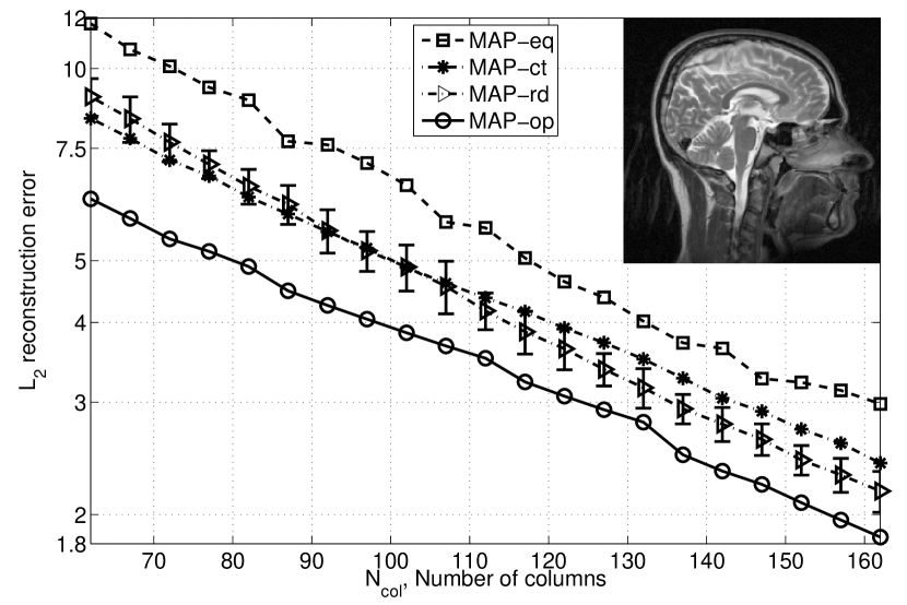
Figure 7: Results for Cartesian undersampling with different measurement designs, on sagittal slice (TSE, TE=92ms). All designs contain 32 central columns. Equispaced [eq]; low-pass [ct]; random with variable density [rd] (averaged over 10 repetitions); optimized by our Bayesian technique [op]. Shown are $\ell_{2}$ distances to $\bm{u}_{\text{true}}$ for MAP reconstruction with the Laplace SLM. Designs optimized on the same data.

Obtained with the same standard sparse reconstruction method (convex $\ell_{1}$ MAP estimation), results for fixed $N_{\text{col}}$ differ “only” in terms of the composition of $\bm{X}$ (recall that scan time grows proportional to $N_{\text{col}}$). Designs chosen by our Bayesian technique substantially outperform all other choices. These results, along with [32, 34], are in stark contrast to claims that independent random sampling is a good way to choose designs for sub-Nyquist reconstruction of real-world images. The improvement of Bayesian optimized over randomly drawn designs is larger for smaller $N_{\text{col}}$. In fact, variable-density sampling does worse than conventional low-pass designs below $1/2$ Nyquist. Similar findings are obtained in [32] for different natural images. In the regime far below the Nyquist limit, it is all the more important to judiciously optimize the design, using criteria informed about realistic images in the first place.

A larger range of results is given in [34]. Even at $1/4$ Nyquist, designs optimized by our method lead to images where most relevant details are preserved. In Figure 7, testing and design optimization is done on the same dataset. The generalization capability of our optimized designs is tested in this larger study, applying them to a range of data from different subjects, different contrasts, and different orientations, achieving improvements on these test sets comparable to what is shown in Figure 7. Finally, we have concentrated on single image slice optimization in our experiments. In realistic MRI experiments, a number of neighbouring slices is acquired in an interleaved fashion. Strong statistical dependencies between slices can be exploited, both in reconstruction and joint design optimization, by combining our framework with structured graphical model message passing [30].

8 Discussion

In this paper, we introduce scalable algorithms for approximate Bayesian inference in sparse linear models, complementing the large body of work on point estimation for these models. If the Bayesian posterior is not just taken for a criterion to be optimized, but as global picture of uncertainty in a reconstruction problem, advanced decision-making problems such as model calibration, feature relevance ranking or Bayesian experimental design can be addressed. We settle a long-standing question for continuous-variable variational Bayesian inference, proving that the relaxation of interest here [17, 23, 11] has the same convexity profile than MAP estimation. Our double loop algorithms are scalable by reduction to common computational problems, penalized least squares optimization and Gaussian covariance estimation (or principal components analysis). The large and growing body of work for the latter, both in theory and algorithms, is put to novel use in our methods. Moreover, the reductions offer valuable insight into similarities and differences between sparse estimation and approximate Bayesian inference, as do our focus on decision-making problems beyond point reconstruction.

We apply our algorithms to the design optimization problem of improving sampling trajectories for magnetic resonance imaging. To the best of our knowledge, this has not been attempted before in the context of sparse nonlinear reconstruction. Ours is the first approximate Bayesian framework for adaptive compressive sensing that scales up to and succeeds on full high-resolution real-world images. Results here are part of a larger MRI study [34], where designs optimized by our Bayesian technique are found to significantly and robustly improve sparse image reconstruction on a wide range of test datasets, for measurements far below the Nyquist limit.

In future work, we will address advanced joint design scenarios, such as MRI sampling optimization for multiple image slices, 3D MRI, and parallel MRI with array coils. Our technique can be sped up along many directions, from algorithmic improvements (advanced algorithms for inner loop optimization, modern Lanczos variants) down to parallel computation on graphics hardware. An important future goal, currently out of reach, is supporting real-time MRI applications by automatic on-line sampling optimization.

Acknowledgments

The MRI application is joint work with Rolf Pohmann and Bernhard Schölkopf, MPI for Biological Cybernetics, Tübingen. We thank Florian Steinke and David Wipf for helpful discussions and input. Supported in part by the IST Programme of the European Community, under the PASCAL Network of Excellence, IST-2002-506778, and the Excellence Initiative of the German research foundation (DFG).

Appendix A Details and Proofs

A.1 Proof of Theorem 1

In this section, we provide a proof of Theorem 1. For notational convenience, we absorb $\sigma^{-2}$ into $\bm{X}^{T}\bm{X}$, by replacing $\bm{X}$ by $\sigma^{-1}\bm{X}$. We begin with part (2). It is well known that $\bm{\pi}\mapsto\log|\tilde{\bm{A}}(\bm{\pi})|$ is concave and nondecreasing for $\bm{\pi}\succ\bm{0}$ [4, Sect. 3.1.5]. Both properties carry over to the extended-value function. The statement follows from the concatenation rules of [4, Sect. 3.2.4].

We continue with part (1). Write $\tilde{\bm{A}}=\tilde{\bm{A}}(f(\bm{\gamma}))$, $\psi_{1}:=\log|\tilde{\bm{A}}|$, $\bm{\Gamma}=\operatorname{diag}\bm{\gamma}$, and $f(\bm{\Gamma})=\operatorname{diag}f(\bm{\gamma})$. First, $\bm{\gamma}\mapsto\psi_{1}$ is the composition of twice continuously differentiable mappings, thus inherits this property. Now, $d\psi_{1}=\operatorname{tr}\bm{S}f^{\prime}(\bm{\Gamma})(d\bm{\Gamma})$, where $\bm{S}:=\bm{B}\tilde{\bm{A}}^{-1}\bm{B}^{T}$, moreover $d^{2}\psi_{1}=-\operatorname{tr}\bm{S}f^{\prime}(\bm{\Gamma})(d\bm{\Gamma})\bm{S}f^{\prime}(\bm{\Gamma})(d\bm{\Gamma})+\operatorname{tr}\bm{S}f^{\prime\prime}(\bm{\Gamma})(d\bm{\Gamma})^{2}=\operatorname{tr}(d\bm{\Gamma})\bm{S}(d\bm{\Gamma})\bm{E}_{1}$, where $\bm{E}_{1}{}:=f^{\prime\prime}(\bm{\Gamma})-f^{\prime}(\bm{\Gamma})\bm{S}f^{\prime}(\bm{\Gamma})$. Since $\bm{S}\succeq\bm{0}$, we have $\bm{S}=\bm{V}\bm{V}^{T}$ for some matrix $\bm{V}$, and $d^{2}\psi_{1}=\operatorname{tr}((d\bm{\Gamma})\bm{V})^{T}\bm{E}_{1}{}(d\bm{\Gamma})\bm{V}$. Now, if $\bm{E}_{1}{}\succeq\bm{0}$, then for $\bm{\gamma}^{(t)}=\bm{\gamma}+t(\Delta\bm{\gamma})$, we have $\psi_{1}^{\prime\prime}(0)=\operatorname{tr}\bm{N}^{T}\bm{E}_{1}{}\bm{N}\geq 0$ for any $\Delta\bm{\gamma}$, where $\bm{N}:=(\operatorname{diag}\Delta\bm{\gamma})\bm{V}$, so that $\psi_{1}$ is convex.

The log-convexity of $f_{i}(\gamma_{i})$ implies that $f_{i}(\gamma_{i})f_{i}^{\prime\prime}(\gamma_{i})\geq(f_{i}^{\prime}(\gamma_{i}))^{2}$ for all $\gamma_{i}$, so that

$$\begin{split}\bm{E}_{1}{}&=f(\bm{\Gamma})^{-1}(f(\bm{\Gamma})f^{\prime\prime}(\bm{\Gamma}))-f^{\prime}(\bm{\Gamma})\bm{S}f^{\prime}(\bm{\Gamma})\succeq f(\bm{\Gamma})^{-1}(f^{\prime}(\bm{\Gamma}))^{2}-f^{\prime}(\bm{\Gamma})\bm{S}f^{\prime}(\bm{\Gamma})\\ &=f^{\prime}(\bm{\Gamma})\left(f(\bm{\Gamma})^{-1}-\bm{S}\right)f^{\prime}(\bm{\Gamma}).\end{split}$$

Therefore, it remains to be shown that $f(\bm{\Gamma})^{-1}-\bm{S}\succeq\bm{0}$. We use the identity

$$\bm{v}^{T}\bm{M}^{-1}\bm{v}=\max_{\bm{x}}2\bm{v}^{T}\bm{x}-\bm{x}^{T}\bm{M}\bm{x},$$ (14)

which holds whenever $\bm{M}\succ\bm{0}$. For any $\bm{r}\in\mathbb{R}^{q}$:

$$\bm{r}^{T}\bm{B}\tilde{\bm{A}}^{-1}\bm{B}^{T}\bm{r}=\max_{\bm{x}}2\bm{r}^{T}\bm{B}\bm{x}-\bm{x}^{T}\left(\bm{X}^{T}\bm{X}+\bm{B}^{T}f(\bm{\Gamma})\bm{B}\right)\bm{x}\leq\max_{\bm{k}=\bm{B}\bm{x}}2\bm{r}^{T}\bm{k}-\bm{k}^{T}f(\bm{\Gamma})\bm{k},$$

using (14) and $\bm{x}^{T}\bm{X}^{T}\bm{X}\bm{x}=\|\bm{X}\bm{x}\|^{2}\geq 0$. Therefore, $\bm{r}^{T}\bm{S}\bm{r}\leq\max_{\bm{k}}2\bm{r}^{T}\bm{k}-\bm{k}^{T}f(\bm{\Gamma})\bm{k}=\bm{r}^{T}f(\bm{\Gamma})^{-1}\bm{r}$, using (14) once more, which implies $f(\bm{\Gamma})^{-1}-\bm{S}\succeq\bm{0}$. This completes the proof of part (1). Since $\bm{A}=\tilde{\bm{A}}(\bm{\gamma}^{-1})$, we can employ this argument with $f_{i}(\gamma_{i})=\gamma_{i}^{-1}$ and $\bm{r}=\bm{\delta}_{i}$ in order to establish part (4).

We continue with part (3). Write $\tilde{\bm{A}}=\tilde{\bm{A}}(f(\bm{\gamma})^{-1})$ and $\psi_{2}:=\bm{1}^{T}(\log f(\bm{\gamma}))+\log|\tilde{\bm{A}}|$. Assume for now that $\bm{X}^{T}\bm{X}\succ\bm{0}$. Let $\bm{B}=(\bm{B}_{<q}^{T}\,\tilde{\bm{b}})^{T}$ (so that $\tilde{\bm{b}}^{T}$ is the last row of $\bm{B}$), and define $\tilde{\bm{A}}_{<q}=\bm{X}^{T}\bm{X}+\bm{B}_{<q}^{T}f(\bm{\Gamma}_{<q})^{-1}\bm{B}_{<q}$, where $f(\bm{\gamma}_{<q})=(f_{i}(\gamma_{i}))_{i<q}\in\mathbb{R}^{q-1}_{+}$. We make use of the well-known determinant identity $|\bm{I}+\bm{v}\bm{v}^{T}|=1+\bm{v}^{T}\bm{v}$. Namely,

$$\begin{split}&\log f_{q}(\gamma_{q})+\log\left|\tilde{\bm{A}}_{<q}+f_{q}(\gamma_{q})^{-1}\tilde{\bm{b}}\tilde{\bm{b}}^{T}\right|\\ =\,&\log f_{q}(\gamma_{q})+\log\left|\tilde{\bm{A}}_{<q}\right|+\log\left|\bm{I}+f_{q}(\gamma_{q})^{-1}(\tilde{\bm{A}}_{<q})^{-1}\tilde{\bm{b}}\tilde{\bm{b}}^{T}\right|\\ =\,&\log\left|\tilde{\bm{A}}_{<q}\right|+\log f_{q}(\gamma_{q})+\log\left(1+f_{q}(\gamma_{q})^{-1}\tilde{\bm{b}}^{T}(\tilde{\bm{A}}_{<q})^{-1}\tilde{\bm{b}}\right)\\ =\,&\log\left|\tilde{\bm{A}}_{<q}\right|+\log\left(f_{q}(\gamma_{q})+\tilde{\bm{b}}^{T}(\tilde{\bm{A}}_{<q})^{-1}\tilde{\bm{b}}\right).\end{split}$$ (15)

Since the extended-value function $\log(\cdot)$ (assigning $-\infty$ to arguments $\leq 0$) is concave and nondecreasing, the concatenation rules of [4, Sect. 3.2.4] imply the concavity of the final term in (15) whenever $f_{q}(\gamma_{q})+\tilde{\bm{b}}^{T}(\tilde{\bm{A}}_{<q})^{-1}\tilde{\bm{b}}$ is concave. We will use induction on $q$, the dimensionality of $\bm{\gamma}$. For $q=1$, $\psi_{2}$ is given by (15) with $\tilde{\bm{A}}_{<1}=\bm{X}^{T}\bm{X}$, and its concavity follows from the concavity of $f_{1}(\gamma_{1})$. For $q>1$, (15) implies

$$\psi_{2}=\bm{1}^{T}(\log f(\bm{\gamma}_{<q}))+\log|\tilde{\bm{A}}_{<q}|+\log\left(f_{q}(\gamma_{q})+\tilde{\bm{b}}^{T}(\tilde{\bm{A}}_{<q})^{-1}\tilde{\bm{b}}\right).$$

Both the sum of the first two terms and $f_{q}(\gamma_{q})$ are concave by assumption, so that the concavity of $\psi_{2}$ is implied by the concavity of $\bm{\gamma}\mapsto\tilde{\bm{b}}^{T}(\tilde{\bm{A}}_{<q})^{-1}\tilde{\bm{b}}$. Using (14), we have

$$\tilde{\bm{b}}^{T}(\tilde{\bm{A}}_{<q})^{-1}\tilde{\bm{b}}=\max_{\bm{x}}2\tilde{\bm{b}}^{T}\bm{x}-\bm{x}^{T}\tilde{\bm{A}}_{<q}\bm{x}=\max_{\bm{x}}2\tilde{\bm{b}}^{T}\bm{x}-\|\bm{X}\bm{x}\|^{2}-\bm{v}^{T}f(\bm{\Gamma}_{<q})^{-1}\bm{v}$$

with $\bm{v}:=\bm{B}_{<q}\bm{x}$. Now, $(\bm{x},\bm{f})\mapsto 2\tilde{\bm{b}}^{T}\bm{x}-\|\bm{X}\bm{x}\|^{2}-\bm{v}^{T}(\operatorname{diag}\bm{f})^{-1}\bm{v}$ is jointly concave for $\bm{f}\succ\bm{0}$ (see proof of Theorem 2), so that $\kappa(\bm{f}):=\tilde{\bm{b}}^{T}\tilde{\bm{A}}_{<q}(\bm{f}^{-1})^{-1}\tilde{\bm{b}}$ is concave for $\bm{f}\succ\bm{0}$ [4, Sect. 3.2.5] (recall that $\tilde{\bm{A}}_{<q}(\bm{f}^{-1})=\bm{X}^{T}\bm{X}+\bm{B}_{<q}^{T}(\operatorname{diag}\bm{f}^{-1})\bm{B}_{<q}$). To finish the argument, we plug in $\bm{f}:=f(\bm{\gamma}_{<q})$ and use the concatenation theorems of [4, Sect. 3.2.4]. What remains to be shown in this context is that $\kappa(\bm{f})$ is nondecreasing in each argument. Pick any $i\in\{{1},\dots,{q}\}$, $\bm{f}\succ\bm{0}$, and any $\Delta>0$. Then,

$$\kappa(\bm{f}+\Delta\bm{\delta}_{i})=\tilde{\bm{b}}^{T}\left(\tilde{\bm{A}}_{<q}(\bm{f}^{-1})-\frac{\Delta}{f_{i}(f_{i}+\Delta)}\bm{b}_{i}\bm{b}_{i}^{T}\right)^{-1}\tilde{\bm{b}}\geq\tilde{\bm{b}}^{T}\tilde{\bm{A}}_{<q}(\bm{f}^{-1})^{-1}\tilde{\bm{b}}=\kappa(\bm{f}),$$

where $\bm{b}_{i}=\bm{B}^{T}\bm{\delta}_{i}$. This concludes the proof of part (3), under the assumption that $\bm{X}^{T}\bm{X}$ is invertible. If $\bm{X}^{T}\bm{X}$ is singular, define $\psi_{2}^{\mathrm{\varepsilon}}$ as above, but with $\bm{X}^{T}\bm{X}\to\bm{X}^{T}\bm{X}+\mathrm{\varepsilon}\bm{I}$. We saw that $\psi_{2}^{\mathrm{\varepsilon}}$ is concave for any $\mathrm{\varepsilon}>0$. For any $\bm{\gamma}\succ\bm{0}$ such that $\psi_{2}(\bm{\gamma})>-\infty$, $\psi_{2}^{\mathrm{\varepsilon}}$ converges uniformly to $\psi_{2}$ on a closed environment of $\bm{\gamma}$ ($\psi_{2}$ and all $\psi_{2}^{\mathrm{\varepsilon}}$ are continuous), so that $\psi_{2}$ is concave at $\bm{\gamma}$. This completes the proof of part (3).

A.2 Proof of Theorem 3

In this section, we provide of proof of Theorem 3. We begin with part (1), focussing on a single potential $i$ and dropping its index. Since $b\neq 0$ is dealt with separately, assume that $t(s)$ is even: $\log t(s)=\tilde{g}(s)=g(s^{2})=g(x)$, where $x=s^{2}$. If $f(x,\gamma):=-x/\gamma-2g(x)$ and $\tilde{f}(s,\gamma):=-s^{2}/\gamma-2\tilde{g}(s)$, then $h(\gamma)=\max_{x\geq 0}f(x,\gamma)$, and $f(x,\gamma)=\tilde{f}(x^{1/2},\gamma)$. It suffices to consider $s\geq 0$. Denote $x_{*}=x_{*}(\gamma):=\operatorname*{argmax}_{x\geq 0}f(x,\gamma)$ (unique, since $g(x)$ is strictly convex). If $\gamma_{0}:=\sup\{\gamma\,|\,f(x,\gamma)\leq-2g(0)\;\forall x\}$ ($\gamma_{0}=0$ for an empty set), then

• $x_{*}=0$, $h(\gamma)=-2g(0)$ for $\gamma\in(0,\gamma_{0}]$

• $x_{*}>0$, $h(\gamma)$ strictly increasing for $\gamma>\gamma_{0}$

Namely, if $\gamma_{0}<\gamma_{1}<\gamma_{2}$, then $x_{*}(\gamma_{1})>0$ by definition of $\gamma_{0}$, and $h(\gamma_{1})=-x_{*}(\gamma_{1})/\gamma_{1}-2g(x_{*}(\gamma_{1}))<-x_{*}(\gamma_{1})/\gamma_{2}-2g(x_{*}(\gamma_{1}))\leq-x_{*}(\gamma_{2})/\gamma_{2}-2g(x_{*}(\gamma_{2}))=h(\gamma_{2})$. Note that $\gamma_{0}>0$ iff $\lim_{\mathrm{\varepsilon}\searrow 0}g^{\prime}(\mathrm{\varepsilon})$ is finite. It suffices to show that $h$ is convex at all $\gamma>\gamma_{0}$, where $x_{*}=s_{*}^{2}>0$.

We use the notation $\tilde{f}_{s}=\partial\tilde{f}/(\partial s)$, functions are evaluated at $(x_{*}=s_{*}^{2},\gamma)$ if nothing else is said. Now, $\tilde{f}_{s}=-2s_{*}/\gamma-2\tilde{g}_{s}(s_{*})=0$, so that $\tilde{g}_{s}(s_{*})=-s_{*}/\gamma$. Next, $g(x)$ is twice continuously differentiable, and $x_{*}=s_{*}^{2}$ at $\gamma$. Therefore, $f_{x}=\partial f/(\partial x)$ is continuously differentiable. Moreover, $g_{x,x}(x)>0$ by the strict convexity of $g(x)$. By the implicit function theorem, $x_{*}(\gamma)$ is continuously differentiable at $\gamma$, and since $h(\gamma)=f(x_{*}(\gamma),\gamma)$, $h^{\prime}(\gamma)$ exists. Moreover, $0=(d/d\gamma)f_{x}(x_{*}(\gamma),\gamma)=f_{x,\gamma}+f_{x,x}\cdot(dx_{*})/(d\gamma)$, so that $(dx_{*})/(d\gamma)=\gamma^{-2}/(2g_{x,x}(x_{*}))>0$: $x_{*}(\gamma)$ is increasing. From $f_{x}=0$, we have that $h^{\prime}(\gamma)=f_{\gamma}=s_{*}^{2}/\gamma^{2}=(\tilde{g}_{s}(s_{*}))^{2}$, since $\tilde{g}_{s}(s_{*})=-s_{*}/\gamma$. Now, $\tilde{g}_{s}(s)$ is nonincreasing by the concavity of $\tilde{g}(s)$, and $\tilde{g}_{s}(s_{*})<0$, so that $s_{*}\mapsto h^{\prime}(\gamma)$ is nondecreasing. Since $s_{*}^{2}=x_{*}$ is increasing in $\gamma$, so is $s_{*}$. Therefore, $\gamma\mapsto h^{\prime}(\gamma)$ is nondecreasing, which means that $h(\gamma)$ is convex for $\gamma>\gamma_{0}$.

The concavity of $\tilde{g}(s)$ is necessary. Suppose that $\tilde{g}_{s,s}(\tilde{s})>0$ for some $\tilde{s}>0$. If $\tilde{x}=\tilde{s}^{1/2}$, $g(x)$ is differentiable at $\tilde{x}$, and if $\tilde{\gamma}=-1/(2g^{\prime}(\tilde{x}))$, then $s_{*}(\tilde{\gamma})=\tilde{s}$. But if $\tilde{g}_{s,s}(s_{*})>0$ at $\tilde{\gamma}$, then $s_{*}\mapsto h^{\prime}(\gamma)$ is decreasing at $s_{*}=\tilde{s}$, and just as above $\gamma\mapsto h^{\prime}(\gamma)$ is decreasing at $\tilde{\gamma}$, so that $h$ is not convex at $\tilde{\gamma}$. This concludes the proof of part (1).

Part (2) is a direct consequence of part (1) and Theorem 2. For the final statement, suppose that $h_{i}^{\prime}(\gamma_{i})$ is decreasing at $\gamma_{i}=\tilde{\gamma_{i}}$. Pick the other coefficients in $\tilde{\bm{\gamma}}\succ\bm{0}$ arbitrary, and choose $m=n=1$, $\bm{y}=\bm{0}$, $\bm{X}=X$, $\bm{B}=\bm{\delta}_{i}$, so that $\phi(\bm{\gamma})-h(\bm{\gamma})=r(\gamma_{i}):=\log(1+X^{2}\gamma_{i})-\log\gamma_{i}$, ignoring additive constants. Consider $\tilde{\phi}(t)=\phi{}(\tilde{\bm{\gamma}}+t\bm{\delta}_{i})$. Since $r^{\prime}(\tilde{\gamma}_{i})=X^{2}/(1+X^{2}\tilde{\gamma}_{i})-1/\tilde{\gamma}_{i}\to 0$ for $X\to\infty$, $\tilde{\phi}^{\prime}(t)$ is decreasing at $t=0$ for large enough $X$, and $\phi$ is not convex at $\tilde{\bm{\gamma}}$.

A.3 Proof of Theorem 4

In this section, we provides proofs related to Section 5. We begin with Theorem 4. For the first part, fix any $\bm{\pi}\succ\bm{0}$, any $i\in\{{1},\dots,{q}\}$, and any $\Delta>0$. If $\bm{b}_{i}=\bm{B}^{T}\bm{\delta}_{i}\neq\bm{0}$, then using the determinant identity previously employed in Appendix A.1, we have

$$\begin{split}\log|\tilde{\bm{A}}(\bm{\pi}+\Delta\bm{\delta}_{i})|&=\log|\tilde{\bm{A}}(\bm{\pi})|+\log\left|\bm{I}+\Delta\tilde{\bm{A}}(\bm{\pi})^{-1}\bm{b}_{i}\bm{b}_{i}^{T}\right|\\ &=\log|\tilde{\bm{A}}(\bm{\pi})|+\log(1+\Delta\bm{b}_{i}^{T}\tilde{\bm{A}}(\bm{\pi})^{-1}\bm{b}_{i})>\log|\tilde{\bm{A}}(\bm{\pi})|,\end{split}$$

since $\bm{b}_{i}^{T}\tilde{\bm{A}}(\bm{\pi})^{-1}\bm{b}_{i}>0$ and $\log(1+x)>0$ for $x>0$. Therefore, $\log|\tilde{\bm{A}}(\bm{\pi})|$ is increasing in each component. Moreover, we have that $\log|\tilde{\bm{A}}(\bm{\pi}+\Delta\bm{\delta}_{i})|\to\infty$ ($\Delta\to\infty$), since $\log(1+x)$ is unbounded above for $x\to\infty$. If $\bm{\pi}_{t}$ is a sequence with $\|\bm{\pi}_{t}\|\to\infty$ and $\bm{\pi}_{t}\succeq\mathrm{\varepsilon}\bm{1}$, there must be some $i\in\{{1},\dots,{q}\}$ such that $(\bm{\pi}_{t})_{i}\to\infty$. If $\tilde{\bm{\pi}}_{t}:=\mathrm{\varepsilon}\bm{1}+((\bm{\pi}_{t})_{i}-\mathrm{\varepsilon})\bm{\delta}_{i}\succeq\bm{\pi}_{t}$, then $\log|\tilde{\bm{A}}(\bm{\pi}_{t})|\geq\log|\tilde{\bm{A}}(\tilde{\bm{\pi}}_{t})|\to\infty$ ($t\to\infty$).

For the second part, recall that

$$\begin{split}&\phi(\bm{\gamma})=\log|\bm{A}|+h(\bm{\gamma})+\min_{\bm{u}}\left\{R(\bm{u},\bm{\gamma})=\sigma^{-2}\|\bm{y}-\bm{X}\bm{u}\|^{2}+\bm{s}^{T}\bm{\Gamma}^{-1}\bm{s}-2\bm{b}^{T}\bm{s}\right\},\\ &-2\log P(\bm{u}|\bm{y})=\min_{\bm{\gamma}\succeq\bm{0}}h(\bm{\gamma})+R(\bm{u},\bm{\gamma})+C_{2},\quad\bm{s}=\bm{B}\bm{u}\end{split}$$

for some constant $C_{2}$. If $\bm{\gamma}_{t}$ is a bounded sequence such that $(\bm{\gamma}_{t})_{i}\to 0$ ($t\to\infty$) for some $i\in\{{1},\dots,{q}\}$, then $\log|\bm{A}(\bm{\gamma}_{t})|=\log|\tilde{\bm{A}}(\bm{\gamma}_{t}^{-1})|\to\infty$. Suppose that $\phi(\bm{\gamma}_{t})$ remains bounded above. Let $\bm{u}_{t}=\operatorname*{argmin}_{\bm{u}}R(\bm{u},\bm{\gamma}_{t})$. Then, $\phi(\bm{\gamma}_{t})-\log|\bm{A}(\bm{\gamma}_{t})|=h(\bm{\gamma}_{t})+R(\bm{u}_{t},\bm{\gamma}_{t})\to-\infty$, so that $-2\log P(\bm{u}_{t}|\bm{y})-C_{2}\leq h(\bm{\gamma}_{t})+R(\bm{u}_{t},\bm{\gamma}_{t})\to-\infty$, in contradiction to the boundedness of the log posterior. This concludes the proof.

Next, assume we run MAP estimation (10) with even super-Gaussian potentials $t_{i}(s_{i})$, so that $|s_{i}|\mapsto-\log t_{i}(s_{i})=-\tilde{g}_{i}(s_{i})$ is concave. As argued in Section 5, any local minimum point $\bm{s}_{*}=\bm{B}\bm{u}_{*}$ is exactly sparse. We show that the corresponding $\bm{\gamma}_{*}$ has the same sparsity pattern: $\gamma_{*,i}=0$ whenever $s_{*,i}=0$. Dropping the index, since $\gamma_{*}\in\operatorname*{argmin}_{\gamma\geq 0}s_{*}^{2}/\gamma+h(\gamma)$, we have to show that $h(\gamma)>h(0)$ for all $\gamma>0$ (or, in terms of Appendix A.2, that $\gamma_{0}=0$). Fix $\gamma>0$, and recall that $h(\gamma)=\max_{s\geq 0}\{\tilde{f}(s,\gamma)=-s^{2}/\gamma-2\tilde{g}(s)\}\geq-2\tilde{g}(0)=h(0)$. Now, $\tilde{f}(s,\gamma)=-2\tilde{g}(s)+O(s^{2})$, $s\searrow 0$, where $-2\tilde{g}(s)$ is concave, nondecreasing and not constant. Therefore, $\lim_{s\searrow 0}\partial\tilde{f}/(\partial s)\in(0,\infty]$, and $\tilde{f}(\tilde{s},\gamma)>\tilde{f}(0,\gamma)$ for some $\tilde{s}>0$, so that $h(\gamma)\geq\tilde{f}(\tilde{s},\gamma)>h(0)$.

A.4 Details for Bounding $\log|\bm{A}|$

In this section, we provide details concerning the $\log|\bm{A}|$ bounds discussed in Section 4.2. Recall that $\tilde{\bm{A}}(\bm{\pi})=\sigma^{-2}\bm{X}^{T}\bm{X}+\bm{B}^{T}(\operatorname{diag}\bm{\pi})\bm{B}$ for $\bm{\pi}\succ\bm{0}$. Define the extended-value extension $g_{1}(\bm{\pi})=\lim_{\bm{d}\searrow\bm{\pi}}\log|\tilde{\bm{A}}(\bm{d})|$, $\bm{\pi}\succeq\bm{0}$, $g_{1}(\bm{\pi})=-\infty$ elsewhere (note that $\log|\tilde{\bm{A}}(\bm{\pi})|$ is continuous). Since $g_{1}$ is lower semicontinuous, and concave for $\bm{\pi}\succ\bm{0}$ (Theorem 1(2)), it is a closed proper concave function. Fenchel duality [26, Sect. 12] implies that $g_{1}(\bm{\pi})=\inf_{\bm{z}_{1}}\bm{z}_{1}^{T}\bm{\pi}-g_{1}^{*}(\bm{z}_{1})$, where $g_{1}^{*}(\bm{z}_{1})=\inf_{\bm{\pi}}\bm{z}_{1}^{T}\bm{\pi}-g_{1}(\bm{\pi})$ is closed concave as well. As $g_{1}(\bm{\pi})$ is unbounded above as $\|\bm{\pi}\|\to\infty$ (Theorem 4), $\bm{z}_{1}^{T}\bm{\pi}-g_{1}(\bm{\pi})$ is unbounded below whenever $z_{1,i}\leq 0$ for any $i$, and $g_{1}^{*}(\bm{z}_{1})=-\infty$ in this case. Moreover, for any $\bm{\pi}\succ\bm{0}$, the corresponding minimizer $\bm{z}_{1,*}$ is given in Section 4.2, so that $g_{1}(\bm{\pi})=\min_{\bm{z}_{1}\succ\bm{0}}\bm{z}_{1}^{T}\bm{\pi}-g_{1}^{*}(\bm{z}_{1})$.

Second, define the extended-value extension $g_{2}(\bm{\gamma})=\lim_{\bm{d}\searrow\bm{\gamma}}\bm{1}^{T}(\log\bm{d})+\log|\tilde{\bm{A}}(\bm{d})|$, $\bm{\gamma}\succeq\bm{0}$, $g_{2}(\bm{\gamma})=-\infty$ elsewhere (note that $\bm{1}^{T}(\log\bm{\pi})+\log|\tilde{\bm{A}}(\bm{\pi})|$ is continuous). Since $g_{2}$ is lower semicontinuous, and concave for $\bm{\gamma}\succ\bm{0}$ (Theorem 1(3)), it is a closed proper concave function. Fenchel duality [26, Sect. 12] implies that $g_{2}(\bm{\gamma})=\inf_{\bm{z}_{2}}\bm{z}_{2}^{T}\bm{\gamma}-g_{2}^{*}(\bm{z}_{2})$, where $g_{2}^{*}(\bm{z}_{2})=\inf_{\bm{\gamma}}\bm{z}_{2}^{T}\bm{\gamma}-g_{2}(\bm{\gamma})$ is closed concave as well. Since $\bm{z}_{2}^{T}\bm{\gamma}-g_{2}(\bm{\gamma})$ is unbounded below whenever $z_{2,i}<0$ for any $i$, we see that $g_{2}^{*}(\bm{z}_{2})=-\infty$ in this case. For any $\bm{\gamma}\succ\bm{0}$, the corresponding minimizer $\bm{z}_{2,*}$ is given in Section 4.2, so that $g_{2}(\bm{\gamma})=\min_{\bm{z}_{2}\succeq\bm{0}}\bm{z}_{2}^{T}\bm{\gamma}-g_{2}^{*}(\bm{z}_{2})$.

A.5 Implicit Computation of $h_{i}$ and $h_{i}^{*}$

Recall from Section 4 and Section 4.3 that our algorithms can be run whenever $h_{i}^{*}(s_{i})$ and its derivatives can be evaluated. For log-concave potentials, these evaluations can be done generically, even if no closed form for $h_{i}(\gamma_{i})$ is available. We focus on a single potential $i$ and drop its index. As noted in Section 4, if $z_{2}=z_{3}=0$, then $h^{*}(s)=-g(z_{1}+s^{2})$. With $p:=z_{1}+s^{2}$, we have that $\theta=-2g^{\prime}(p)s-b$, $\rho=-4g^{\prime\prime}(p)s^{2}-2g^{\prime}(p)$. With a view to Appendix A.7, $\tilde{\theta}=-2g^{\prime}(p)$, $p=z_{1}+\|\bm{s}\|^{2}$, and $\kappa=2[g^{\prime\prime}(p)]^{1/2}$.

If $z_{2}\neq 0$ (and $t(s)$ log-concave), we have to employ scalar convex minimization. We require $h^{*}(s)=\frac{1}{2}\min_{\gamma}k(x,\gamma)$, $k:=(z_{1}+x)/\gamma+z_{2}\gamma-z_{3}\log\gamma+h(\gamma)$, $x=s^{2}$, as well as $\theta=(h^{*})^{\prime}(s)$ and $\rho=(h^{*})^{\prime\prime}(s)$. Let $\gamma_{*}=\operatorname*{argmin}k(x,\gamma)$. Assuming for now that $h$ and its derivatives are available, $\gamma_{*}$ is found by univariate Newton minimization, where $\gamma^{2}k_{\gamma}=-(z_{1}+x)-z_{3}\gamma+\gamma^{2}(z_{2}+h^{\prime}(\gamma))$, $\gamma^{3}k_{\gamma,\gamma}=2(z_{1}+x)+\gamma z_{3}+\gamma^{3}h^{\prime\prime}(\gamma)$. Now, $k_{\gamma}=0$ (always evaluated at $(x,\gamma_{*})$), so that $\theta=(h^{*})^{\prime}(s)=s/\gamma_{*}$. Moreover, $0=(d/ds)k_{\gamma}=k_{s,\gamma}+k_{\gamma,\gamma}\cdot(d\gamma_{*})/(ds)$, so that $\rho=(h^{*})^{\prime\prime}(s)=\gamma_{*}^{-1}(1-s\gamma_{*}^{-1}(d\gamma_{*})/(ds))=\gamma_{*}^{-1}(1-2x/(\gamma_{*}^{3}k_{\gamma,\gamma}(x,\gamma_{*})))$. With a view to Appendix A.7, $\tilde{\theta}=1/\gamma_{*}$ and $\kappa=[2/(\gamma_{*}^{4}k_{\gamma,\gamma}(x,\gamma_{*}))]^{1/2}$ (note that $\tilde{\theta}\geq\rho$).

By Fenchel duality, $h(\gamma)=-\min_{x}l(x,\gamma)$, $l:=x/\gamma+2g(x)$, where $g(x)$ is strictly convex and decreasing. We need methods to evaluate $g(x)$ and its first and second derivative (note that $g^{\prime\prime}(x)>0$). The minimizer $x_{*}=x_{*}(\gamma)$ is found by convex minimization once more, started from the last recently found $x_{*}$ for this potential. Note that $x_{*}=0$ iff $\gamma\leq\gamma_{0}:=-1/(2g^{\prime}(0))$ (where $\gamma_{0}=0$ if $g^{\prime}(x)\to-\infty$ as $x\to 0$), which has to be checked up front. Given $x_{*}$, we have that $\gamma h(\gamma)=-x_{*}-2\gamma g(x_{*})$. Since $l_{x}=0$ for $\gamma>\gamma_{0}$ (always evaluated at $(x_{*},\gamma)$), then $\gamma^{2}h^{\prime}(\gamma)=-\gamma^{2}l_{\gamma}=x_{*}$ (this holds even if $l_{x}>0$ and $x_{*}=0$). Moreover, if $x_{*}>0$ (for $\gamma>\gamma_{0}$), then $(d/d\gamma)l_{x}(x_{*},\gamma)=0$, so that $(dx_{*})/(d\gamma)=\gamma^{-2}/(2g^{\prime\prime}(x_{*}))$, and $\gamma^{3}h^{\prime\prime}(\gamma)=(2\gamma g^{\prime\prime}(x_{*}))^{-1}-2x_{*}$. If $x_{*}=0$ and $l_{x}>0$, then $x_{*}(\tilde{\gamma})=0$ for $\tilde{\gamma}$ close to $\gamma$, so that $h^{\prime\prime}(\gamma)=0$. A critical case is $x_{*}=0$ and $l_{x}=0$, which happens for $\gamma=\gamma_{0}>0$: $h^{\prime\prime}(\gamma)$ does not exist at this point in general. This is not a problem for our code, since we employ a robust Newton/bisection search for $\gamma_{*}$. If $\gamma>\gamma_{*}$, but is very close, note that $(dx_{*})/(d\gamma)\approx\xi_{0}/\gamma$ with $\xi_{0}:=-g^{\prime}(0)/g^{\prime\prime}(0)$, therefore $x_{*}(\gamma)\approx\int_{\gamma_{0}}^{\gamma}\xi_{0}/t\,dt=\xi_{0}(\log\gamma-\log\gamma_{0})$. We use $\gamma^{2}h^{\prime}(\gamma)=x_{*}\approx\xi_{0}(\log\gamma-\log\gamma_{0})$ and $\gamma^{3}h^{\prime\prime}(\gamma)\approx\xi_{0}-2x_{*}$ in this case.

A.6 Details for Specific Potentials

Our algorithms are configured by the dual functions $h_{i}(\gamma_{i})$ for each non-Gaussian $t_{i}(s_{i})$, and the inner loops require $h_{i}^{*}(s_{i})$ and its derivatives (see (12), and recall that for each $i$, either $z_{1,i}>0$ and $z_{3,i}=0$, or $z_{1,i}=0$ and $z_{2,i}>0,z_{3,i}=1$). In this section, we show how these are computed for the potentials used in this paper. We use the notation of Appendix A.5, focus on a single potential $i$ and drop its index.

Laplace Potentials

These are $t(s)=\exp(-\tau|s|)$, $\tau>0$, so that $g(x)=\tau x^{1/2}$. We have that $h(\gamma)=h_{\cup}(\gamma)=\tau^{2}\gamma$, so that $k(x,\gamma)=(z_{1}+x)/\gamma+(z_{2}+\tau^{2})\gamma-z_{3}\log\gamma$. The stationary equation for $\gamma_{*}$ is $(z_{2}+\tau^{2})\gamma^{2}-z_{3}\gamma-(z_{1}+x)=0$. If $z_{3}=0$ (bounding type A), this is just a special case of Appendix A.5. With $p:=z_{1}+x$, $q:=(z_{2}+\tau^{2})^{1/2}$, we have that $\gamma_{*}=p^{1/2}/q$, $h^{*}(s)=qp^{1/2}$, and $\theta=(h^{*})^{\prime}(s)=qp^{-1/2}s$, $\rho=(h^{*})^{\prime\prime}(s)=qz_{1}p^{-3/2}$. With a view to Appendix A.7, $\tilde{\theta}=qp^{-1/2}$ and $\kappa=[qp^{-3/2}]^{1/2}$.

If $z_{3}=1$ (bounding type B), note that $z_{1}=0$, $z_{2}>0$. Let $q:=2(z_{2}+\tau^{2})$, $p:=(1+2qx)^{1/2}$. Then, $\gamma_{*}=(p+1)/q$, and $k(x,\gamma_{*})=p-\log(p+1)+\log q$ after some algebra, so that $h^{*}(s)=\frac{1}{2}(p-\log(p+1)+\log q)$. With $dp/(ds)=2qp^{-1}s$, we have $\theta=qs/(p+1)$, $\rho=q/(p(p+1))$. With a view to Appendix A.7, $\tilde{\theta}=q/(p+1)$. Using $p^{2}-1=2xq$, some algebra gives $\kappa=(2/p)^{1/2}q/(p+1)=(2/p)^{1/2}\tilde{\theta}$.

Student’s $t$ Potentials

These are $t(s)=(1+(\tau/\nu)x)^{-(\nu+1)/2}$, $\nu>0$, $\tau>0$. If $\alpha:=\nu/\tau$, the critical point of Appendix A.2 is $\gamma_{0}:=\alpha/(\nu+1)$, and $h(\gamma)=[\alpha/\gamma+(\nu+1)\log\gamma+C]\mathrm{I}_{\{\gamma\geq\gamma_{0}\}}$ with $C:=-(\nu+1)(\log\gamma_{0}+1)$. $h(\gamma)$ is not convex. We choose a decomposition such that $h_{\cup}(\gamma)$ is convex and twice continuously differentiable, ensuring that $h^{*}(s)$ is continuously differentiable, and the inner loop optimization runs smoothly. Since $h(\gamma)$ does not have a second derivative at $\gamma_{0}$, neither has $h_{\cap}(\gamma)$.

$$\begin{split}h_{\cap}(\gamma)&=\left\{\begin{array}[]{ll}(\nu+1-z_{3})\log\gamma&|\;\gamma\geq\gamma_{0}\\ (2(\nu+1)-z_{3})\log\gamma-a(\gamma-\gamma_{0})-b&|\;\gamma<\gamma_{0}\end{array}\right.,\\ h_{\cup}(\gamma)&=\left\{\begin{array}[]{ll}\alpha/\gamma+C&|\;\gamma\geq\gamma_{0}\\ -2(\nu+1)\log\gamma+a(\gamma-\gamma_{0})+b&|\;\gamma<\gamma_{0}\end{array}\right.,\end{split}$$

where $b:=(\nu+1)\log\gamma_{0}$, $a:=(\nu+1)/\gamma_{0}$. Here, the $-z_{3}\log\gamma$ term of $k(x,\gamma)$ is folded into $h_{\cap}(\gamma)$.

We follow Appendix A.5 in determining $h^{*}(s)$ and its derivatives, but solve for $\gamma_{*}$ directly. Note that $z_{2}>0$ even if $z_{3}=0$ (bounding type A), due to the Fenchel bound on $h_{\cap}(\gamma)$. We minimize $k(x,\gamma)$ for $\gamma\geq\gamma_{0}$, $\gamma<\gamma_{0}$ respectively and pick the minimum. For $\gamma\geq\gamma_{0}$: $k(x,\gamma)=(z_{1}+\alpha+x)/\gamma+z_{2}\gamma+C$, whose minimum point $\gamma_{*,1}:=[(z_{1}+\alpha+x)/z_{2}]^{1/2}$ is a candidate if $\gamma_{*,1}\geq\gamma_{0}$, with $k(x,\gamma_{*,1})=2[z_{2}(z_{1}+\alpha+x)]^{1/2}+C$. For $\gamma<\gamma_{0}$: $k(x,\gamma)=(z_{1}+x)/\gamma+(z_{2}+a)\gamma-2(\nu+1)\log\gamma+b-a\gamma_{0}$, with minimum point $\gamma_{*,2}:=[\nu+1+((\nu+1)^{2}+(z_{2}+a)(z_{1}+x))^{1/2}]/(z_{2}+a)<\gamma_{0}$. If $z_{2}\leq a$, then $\gamma_{*,2}\geq\gamma_{0}$ (not a candidate). This can be tested up front. If $c:=(z_{2}+a)(z_{1}+x)$, $d:=((\nu+1)^{2}+c)^{1/2}\geq\nu+1$, then $k(x,\gamma_{*,2})=c/(\nu+1+d)+d+(\nu+1)[2\log(z_{2}+a)-2\log(\nu+1+d)+\log\gamma_{0}]=2d+(\nu+1)[2\log(z_{2}+a)-2\log(\nu+1+d)+\log\gamma_{0}-1]$. Now, $\theta$ and $\rho$ are computed as in Appendix A.5 ($h(\gamma)$ there is $h_{\cup}(\gamma)$ here, and $z_{3}=0$, since this is folded into $h_{\cap}$ here), where $\gamma_{*}^{3}h_{\cup}^{\prime\prime}(\gamma_{*})=2\alpha$ for $\gamma_{*}\geq\gamma_{0}$, and $\gamma_{*}^{3}h_{\cup}^{\prime\prime}(\gamma_{*})=2(\nu+1)\gamma_{*}$ for $\gamma_{*}<\gamma_{0}$.

Bernoulli Potentials

These are $t(s)=(1+e^{-y\tau s})^{-1}=e^{y\tau s/2}(2\cosh v)^{-1}$, $v:=(y\tau/2)x^{1/2}=(y\tau/2)|s|$. They are not even, $b=y\tau/2$. While $h(\gamma)$ is not known analytically, we can plug in these expressions into the generic setup of Appendix A.5. Namely, $g(x)=-\log(\cosh v)-\log 2$, so that $g^{\prime}(x)=-C(\tanh v)/v$, $g^{\prime\prime}(x)=(C/2)x^{-1}((\tanh v)/v+\tanh^{2}v-1)$, $C:=(y\tau/2)^{2}/2$. For $x$ close to zero, we use $\tanh v=v-v^{3}/3+2v^{5}/15+O(v^{7})$ for these computations. Moreover, $\gamma_{0}=1/(2C)$ and $\xi_{0}=3/(2C)$.

A.7 Group Potentials

An extension of our framework to group potentials $t_{i}(\|\bm{s}_{i}\|)$ is described in Section 4.5. Recall the details about the IRLS algorithm from Section 4.3. For group potentials, the inner Hessian is not diagonal anymore, but of similarly simple form developed here. $h_{i}^{*}(s_{i})$ becomes $h_{i}^{*}(\|\bm{s}_{i}\|)$, and $x_{i}=\|\bm{s}_{i}\|^{2}$. If $\theta_{i}$, $\rho_{i}$ are as in Section 4.3, $ds_{i}\to d\|\bm{s}_{i}\|$, and $\tilde{\theta}_{i}:=\theta_{i}/\|\bm{s}_{i}\|$, we have that $\nabla_{\bm{s}_{i}}h_{i}^{*}=\tilde{\theta}_{i}\bm{s}_{i}$, since $\nabla_{\bm{s}_{i}}\|\bm{s}_{i}\|=\bm{s}_{i}/\|\bm{s}_{i}\|$. Therefore, the gradient $\bm{\theta}$ is given by $\bm{\theta}_{i}=\tilde{\theta}_{i}\bm{s}_{i}$. Moreover,

$$\nabla\nabla_{\bm{s}_{i}}h_{i}^{*}=\tilde{\theta}_{i}\bm{I}-(\tilde{\theta}_{i}-\rho_{i})\|\bm{s}_{i}\|^{-2}\bm{s}_{i}\bm{s}_{i}^{T}.$$

For simplicity of notation, assume that all $\bm{s}_{i}$ have the same dimensionality. From Appendix A.5, we see that $\tilde{\theta}_{i}\geq\rho_{i}$. Let $\kappa_{i}:=(\tilde{\theta}_{i}-\rho_{i})^{1/2}/\|\bm{s}_{i}\|$, and $\hat{\bm{s}}:=((\operatorname{diag}\bm{\kappa})\otimes\bm{I})\bm{s}$. The Hessian w.r.t. $\bm{s}$ is

$$\bm{H}^{(s)}=(\operatorname{diag}\tilde{\bm{\theta}})\otimes\bm{I}-\sum_{i}\bm{w}_{i}\bm{w}_{i}^{T},\quad\bm{w}_{i}=(\bm{\delta}_{i}\bm{\delta}_{i}^{T}\otimes\bm{I})\hat{\bm{s}}.$$

If $\bm{w}$ is given by $w_{i}=\hat{\bm{s}}_{i}^{T}\bm{v}_{i}$, then $\bm{H}^{(s)}\bm{v}=((\operatorname{diag}\tilde{\bm{\theta}})\otimes\bm{I})\bm{v}-((\operatorname{diag}\bm{w})\otimes\bm{I})\hat{\bm{s}}$. The system matrix for the Newton direction is $\sigma^{-2}\bm{X}^{T}\bm{X}+\bm{B}^{T}\bm{H}^{(s)}\bm{B}$. For numerical reasons, $\tilde{\theta}_{i}$ and $\kappa_{i}$ should be computed directly, rather than via $\theta_{i}$, $\rho_{i}$.

If $\bm{s}_{i}\in\mathbb{R}^{2}$, we can avoid the subtraction in computing $\bm{H}^{(s)}\bm{v}$ and gain numerical stability. Namely, $\nabla\nabla_{\bm{s}_{i}}h_{i}^{*}=\rho_{i}\bm{I}+\kappa_{i}^{2}\left(\|\bm{s}_{i}\|^{2}\bm{I}-\bm{s}_{i}\bm{s}_{i}^{T}\right)$. Since $\|\bm{s}_{i}\|^{2}\bm{I}-\bm{s}_{i}\bm{s}_{i}^{T}=\bm{M}\bm{s}_{i}(\bm{M}\bm{s}_{i})^{T}$, $\bm{M}=\bm{\delta}_{2}\bm{\delta}_{1}^{T}-\bm{\delta}_{1}\bm{\delta}_{2}^{T}$, if we redefine $\hat{\bm{s}}:=((\operatorname{diag}\bm{\kappa})\otimes(\bm{\delta}_{2}\bm{\delta}_{1}^{T}-\bm{\delta}_{1}\bm{\delta}_{2}^{T}))\bm{s}$, then

$$\bm{H}^{(s)}\bm{v}=((\operatorname{diag}\bm{\rho})\otimes\bm{I})\bm{v}+((\operatorname{diag}\bm{w})\otimes\bm{I})\hat{\bm{s}},\quad\bm{w}=\left(\hat{\bm{s}}_{i}^{T}\bm{v}_{i}\right).$$

References

- [1] H. Attias. A variational Bayesian framework for graphical models. In S. Solla, T. Leen, and K.-R. Müller, editors, Advances in Neural Information Processing Systems 12, pages 209–215. MIT Press, 2000.
- [2] C. Bekas, E. Kokiopoulou, and Y. Saad. Computation of large invariant subspaces using polynomial filtered Lanczos iterations. SIAM J. Mat. Anal. Appl., 30(1):397–418, 2008.
- [3] J. Bioucas-Dias and M. Figueiredo. Two-step iterative shrinkage/thresholding algorithms for image restoration. IEEE Transactions on Image Processing, 16(12):2992–3004, 2007.
- [4] S. Boyd and L. Vandenberghe. Convex Optimization. Cambridge University Press, 2002.
- [5] A. Bruckstein, D. Donoho, and M. Elad. From sparse solutions of systems of equations to sparse modeling of signals and images. SIAM Review, 51(1):34–81, 2009.
- [6] E. Candès, J. Romberg, and T. Tao. Robust uncertainty principles: Exact signal reconstruction from highly incomplete frequency information. IEEE Transactions on Information Theory, 52(2):489–509, 2006.
- [7] H. Chang, Y. Weiss, and W. Freeman. Informative sensing. Technical Report 0901.4275v1 [cs.IT], ArXiv, 2009.
- [8] A. Dempster, N. Laird, and D. Rubin. Maximum likelihood from incomplete data via the EM algorithm. Journal of Roy. Stat. Soc. B, 39:1–38, 1977.
- [9] D. Donoho. Compressed sensing. IEEE Transactions on Information Theory, 52(4):1289–1306, 2006.
- [10] D. Donoho and M. Elad. Optimally sparse representation in general (nonorthogonal) dictionaries via minimization. Proc. Natl. Acad. Sci. USA, 100:2197–2202, 2003.
- [11] M. Girolami. A variational method for learning sparse and overcomplete representations. Neural Computation, 13:2517–2532, 2001.
- [12] T. Goldstein and S. Osher. The split Bregman method for L1 regularized problems. SIAM Journal of Imaging Sciences, 2(2):323–343, 2009.
- [13] G. Golub and C. Van Loan. Matrix Computations. Johns Hopkins University Press, 3rd edition, 1996.
- [14] P. Green. Iteratively reweighted least squares for maximum likelihood estimation, and some robust and resistant alternatives. Journal of Roy. Stat. Soc. B, 46(2):149–192, 1984.
- [15] N. Halko, P. Martinsson, and J. Tropp. Finding structure with randomness: Stochastic algorithms for constructing approximate matrix decompositions. Technical Report 0909.4061v1 [math.NA], ArXiv, 2009.
- [16] J. Haupt, R. Castro, and R. Nowak. Distilled sensing: Selective sampling for sparse signal recovery. In D. van Dyk and M. Welling, editors, Workshop on Artificial Intelligence and Statistics 12, pages 216–223, 2008.
- [17] T. Jaakkola. Variational Methods for Inference and Estimation in Graphical Models. PhD thesis, Massachusetts Institute of Technology, 1997.
- [18] S. Ji and L. Carin. Bayesian compressive sensing and projection optimization. In Z. Ghahramani, editor, International Conference on Machine Learning 24. Omni Press, 2007.
- [19] M. Lustig, D. Donoho, and J. Pauly. Sparse MRI: The application of compressed sensing for rapid MR imaging. Magnetic Resonance in Medicine, 58(6):1182–1195, 2007.
- [20] D. Malioutov, J. Johnson, and A. Willsky. Low-rank variance estimation in large-scale GMRF models. In Proceedings of ICASSP, 2006.
- [21] N. Meinshausen and P. Buehlmann. Stability selection. Technical Report 0809.2932v2 [stat.ME], ArXiv, 2009. To appear in JRSS B.
- [22] H. Nickisch and M. Seeger. Convex variational Bayesian inference for large scale generalized linear models. In L. Bottou and M. Littman, editors, International Conference on Machine Learning 26, pages 761–768. Omni Press, 2009.
- [23] J. Palmer, D. Wipf, K. Kreutz-Delgado, and B. Rao. Variational EM algorithms for non-Gaussian latent variable models. In Y. Weiss, B. Schölkopf, and J. Platt, editors, Advances in Neural Information Processing Systems 18. MIT Press, 2006.
- [24] B. Parlett and D. Scott. The Lanczos algorithm with selective orthogonalization. Mathematics of Computation, 33(145):217–238, 1979.
- [25] B. Rao, K. Engan, S. Cotter, J. Palmer, and K. Kreutz-Delgado. Subset selection in noise based on diversity measure minimization. IEEE Transactions on Signal Processing, 51(3):760–770, 2003.
- [26] R. Rockafellar. Convex Analysis. Princeton University Press, 1970.
- [27] M. Schneider and A. Willsky. Krylov subspace estimation. SIAM Journal on Scientific Computing, 22(5):1840–1864, 2001.
- [28] M. Seeger. Bayesian inference and optimal design for the sparse linear model. Journal of Machine Learning Research, 9:759–813, 2008.
- [29] M. Seeger. Sparse linear models: Variational approximate inference and Bayesian experimental design. Journal of Physics: Conference Series, 197(012001), 2009.
- [30] M. Seeger. Speeding up magnetic resonance image acquisition by Bayesian multi-slice adaptive compressed sensing. In Y. Bengio, D. Schuurmans, J. Lafferty, C. K. I. Williams, and A. Culotta, editors, Advances in Neural Information Processing Systems 22, pages 1633–1641, 2009.
- [31] M. Seeger. Gaussian covariance and scalable variational inference. In J. Fürnkranz and T. Joachims, editors, International Conference on Machine Learning 27. Omni Press, 2010.
- [32] M. Seeger and H. Nickisch. Compressed sensing and Bayesian experimental design. In A. McCallum, S. Roweis, and R. Silva, editors, International Conference on Machine Learning 25. Omni Press, 2008.
- [33] M. Seeger, H. Nickisch, R. Pohmann, and B. Schölkopf. Bayesian experimental design of magnetic resonance imaging sequences. In D. Koller, D. Schuurmans, Y. Bengio, and L. Bottou, editors, Advances in Neural Information Processing Systems 21, pages 1441–1448. MIT Press, 2009.
- [34] M. Seeger, H. Nickisch, R. Pohmann, and B. Schölkopf. Optimization of k-space trajectories for compressed sensing by Bayesian experimental design. Magnetic Resonance in Medicine, 63(1):116–126, 2010.
- [35] E. Simoncelli. Modeling the joint statistics of images in the Wavelet domain. In Proceedings 44th SPIE, pages 188–195, 1999.
- [36] F. Steinke, M. Seeger, and K. Tsuda. Experimental design for efficient identification of gene regulatory networks using sparse Bayesian models. BMC Systems Biology, 1(51), 2007.
- [37] R. Tibshirani. Regression shrinkage and selection via the Lasso. Journal of Roy. Stat. Soc. B, 58:267–288, 1996.
- [38] M. Tipping. Sparse Bayesian learning and the relevance vector machine. Journal of Machine Learning Research, 1:211–244, 2001.
- [39] M. Tipping and A. Faul. Fast marginal likelihood maximisation for sparse Bayesian models. In C. Bishop and B. Frey, editors, Workshop on Artificial Intelligence and Statistics 9, 2003. Electronic Proceedings (ISBN 0-9727358-0-1).
- [40] J. Tropp. Algorithms for simultaneous sparse approximation. Part II: Convex relaxation. Signal Processing, 86:589–602, 2006.
- [41] M. Wainwright, E. Sudderth, and A. Willsky. Tree-based modeling and estimation of Gaussian processes on graphs with cycles. In T. Leen, T. Dietterich, and V. Tresp, editors, Advances in Neural Information Processing Systems 13, pages 661–667. MIT Press, 2001.
- [42] M. J. Wainwright and M. I. Jordan. Graphical models, exponential families, and variational inference. Foundations and Trends in Machine Learning, 1(1–2):1–305, 2008.
- [43] D. Wipf and S. Nagarajan. A new view of automatic relevance determination. In J. Platt, D. Koller, Y. Singer, and S. Roweis, editors, Advances in Neural Information Processing Systems 20. MIT Press, 2008.
- [44] D. Wipf and S. Nagarajan. Latent variable Bayesian models for promoting sparsity. Submitted, 2010.
- [45] G. Wright. Magnetic resonance imaging: From basic physics to imaging principles. IEEE Signal Processing Magazine, 14(1):56–66, 1997.
- [46] S. Wright, R. Nowak, and M. Figueiredo. Sparse reconstruction by separable approximation. IEEE Transactions on Signal Processing, 57(7):2479–2493, 2009.
- [47] M. Yuan and Y. Lin. Model selection and estimation in regression with grouped variables. Journal of Roy. Stat. Soc. B, 68(1):49–67, 2006.
- [48] A. Yuille and A. Rangarajan. The concave-convex procedure. Neural Computation, 15(4):915–936, 2003.