Stackelberg Contention Games in Multiuser Networks

Abstract

Interactions among selfish users sharing a common transmission channel can be modeled as a non-cooperative game using the game theory framework. When selfish users choose their transmission probabilities independently without any coordination mechanism, Nash equilibria usually result in a network collapse. We propose a methodology that transforms the non-cooperative game into a Stackelberg game. Stackelberg equilibria of the Stackelberg game can overcome the deficiency of the Nash equilibria of the original game. A particular type of Stackelberg intervention is constructed to show that any positive payoff profile feasible with independent transmission probabilities can be achieved as a Stackelberg equilibrium payoff profile. We discuss criteria to select an operating point of the network and informational requirements for the Stackelberg game. We relax the requirements and examine the effects of relaxation on performance.

1 Introduction

In wireless communication networks, multiple users often share a common channel and contend for access. To resolve the contention problem, many different medium access control (MAC) protocols have been devised and used. Recently, the selfish behavior of users in MAC protocols has been studied using game theory. There have been attempts to understand the existing MAC protocols as the local utility maximizing behavior of selfish users by reverse-engineering the current protocols (e.g., [1]). It has also been investigated whether existing protocols are vulnerable to the existence of selfish users who pursue their self-interest in a non-cooperative manner. Non-cooperative behavior often leads to inefficient outcomes. For example, in the 802.11 distributed MAC protocol, DCF, and its enhanced version, EDCF, competition among selfish users can lead to an inefficient use of the shared channel in Nash equilibria [2]. Similarly, a prisoner’s dilemma phenomenon arises in a non-cooperative game for a generalized version of slotted-Aloha protocols [3].

In general, if a game has Nash equilibria yielding low payoffs for the players, it will be desirable for them to transform the game to extend the set of equilibria to include better outcomes [4]. The same idea can be applied to the game played by selfish users who compete for access to a common medium. If competition among selfish users brings about a network collapse, then it is beneficial for them to design a device which provides incentives to behave cooperatively. Game theory [4] discusses three types of transformation: 1) games with contracts, 2) games with communication, and 3) repeated games.

A game is said to be with contracts if the players of the game can communicate and bargain with each other, and enforce the agreement with a binding contract. The main obstacle to apply this approach to wireless networking is the distributed nature of wireless networks. To reach an agreement, users should know the network system and be able to communicate with each other. They should also be able to enforce the agreed plan.

A game with communication is the one in which players can communicate with each other through a mediator but they cannot write a binding contract. In this case, a correlated equilibrium is predicted to be played. [5] studies correlated equilibria using a coordination mechanism in a slotted Aloha-type scenario. Unlike the first approach, this does not require that the actions of players be enforceable. However, to apply this approach to the medium access problem, signals need to be conveyed from a mediator to all users, and users need to know the correct meanings of the signals.

A repeated game is a dynamic game in which the same game is played repeatedly by the same players over finite or infinite periods. Repeated interactions among the same players enable them to sustain cooperation by punishing deviations in subsequent periods. A main challenge of applying the idea of repeated games to wireless networks is that the users should keep track of their past observations and be able to detect deviations and to coordinate their actions in order to punish deviating users.

Besides the three approaches above, another approach widely applied to communication networks is pricing [6]. A central entity charges prices to users in order to control their utilization of the network. Nash equilibria with pricing schemes in an Aloha network are analyzed in [7, 8]. Implementing a pricing scheme requires the central entity to have relevant system information as well as users’ benefits and costs, which are often their private information. Eliciting private information often results in an efficiency loss in the presence of the strategic behavior of users as shown in [9]. Even in the case where the entity has all the relevant information, prices need to be computed and communicated to the users.

In this paper, we propose yet another approach using a Stackelberg game. We introduce a network manager as an additional user and make him access the medium according to a certain rule. Unlike the Stackelberg game of [10] in which the manager (the leader) chooses a certain strategy before users (followers) make their decisions, in the proposed Stackelberg game he sets an intervention rule first and then implements his intervention after users choose their strategies. Alternatively, the proposed Stackelberg game can be considered as a generalized Stackelberg game in which there are multiple leaders (users) and a single follower (the manager) and the leaders know the response of the follower to their decisions correctly. With appropriate choices of intervention rules, the manager can shape the incentives of users in such a way that their selfish behavior results in cooperative outcomes.

In the context of cognitive radio networks, [11] proposes a related Stackelberg game in which the owner of a licensed frequency band (the leader) can charge a virtual price for using the frequency band to cognitive radios (followers). The virtual price signals the extent to which cognitive radios can exploit the licensed frequency band. However, since prices are virtual, selfish users may ignore prices when they make decisions if they can gain by doing so. On the contrary, in the Stackelberg game of this paper, the intervention of the manager is not virtual but it results in the reduction of throughput, which selfish users care about for sure. Hence, the intervention method provides better grounds for the network manager to deal with the selfish behavior of users.

[12] and [13] use game theoretic models to study random access. Their approach is to capture the information and implementation constraints using the game theoretic framework and to specify utility functions so that a desired operating point is achieved at a Nash equilibrium. If conditions under which a certain type of dynamic adjustment play converges to the Nash equilibrium are met, such a strategy update mechanism can be used to derive a distributed algorithm that converges to the desired operating point. However, this control-theoretic approach to game theory assumes that users are obedient. In this paper, our main concern is about the selfish behavior of users who have innate objectives. Because we start from natural utility functions and affect them by devising an intervention scheme, we are in a better position to deal with selfish users. Furthermore, the idea of intervention can potentially lead to a distributed algorithm to achieve a desired operating point.

By formulating the medium access problem as a non-cooperative game, we show the following main results:

1. Because the Nash equilibria of the non-cooperative game are inefficient and/or unfair, we transform the original game into a Stackelberg game, in which any feasible outcome with independent transmission probabilities can be achieved as a Stackelberg equilibrium.

2. A particular form of a Stackelberg intervention strategy, called total relative deviation (TRD)-based intervention, is constructed and used to achieve any feasible outcome with independent transmission probabilities.

3. The additional amount of information flows required for the transformation is relatively moderate, and it can be further reduced without large efficiency losses.

The rest of this paper is organized as follows. Section 2 introduces the model and formulates it as a non-cooperative game called the contention game. Nash equilibria of the contention game are characterized, and it is shown that they typically yield suboptimal performance. In Section 3, we transform the contention game into another related game called the Stackelberg contention game by introducing an intervening manager. We show that the manager can implement any transmission probability profile as a Stackelberg equilibrium using a class of intervention functions. Section 4 discusses natural candidates for the target transmission probability profile selected by the manager. In Section 5, we discuss the flows of information required for our results and examine the implications of some relaxations of the requirements on performance. Section 6 provides numerical results, and Section 7 concludes the paper.

2 Contention Game Model

We consider a simple contention model in which multiple users share a communication channel as in [14]. A user represents a transmitter-receiver pair. Time is divided into slots of the same duration. Every user has a packet to transmit and can send the packet or wait. If there is only one transmission, the packet is successfully transmitted within the time slot. If more than one user transmits a packet simultaneously in a slot, a collision occurs and no packet is transmitted.

We summarize the assumptions of our contention model.

1. A fixed set of users interacts over a given period of time (or a session).

2. Time is divided into multiple slots, and slots are synchronized.

3. A user always has a packet to transmit in every slot.

4. The transmission of a packet is completed within a slot.

5. A user transmits its packet with the same probability in every slot. There is no adjustment in the transmission probabilities during the session. This excludes coordination among users, for example, using time division multiplexing.

6. There is no cost of transmitting a packet.

We formulate the medium access problem as a non-cooperative game to analyze the behavior of selfish users. We denote the set of users by $N=\{1,\ldots,n\}$. Because we assume that a user uses the same transmission probability over the entire session, the strategy of a user is its transmission probability, and we denote the strategy of user $i$ by $p_{i}$ and the strategy space of user $i$ by $P_{i}=[0,1]$ for all $i\in N$.

Once the users decide their transmission probabilities, a strategy profile can be constructed. The users transmit their packets independently according to their transmission probabilities, and thus the strategy profile determines the probability of a successful transmission by user $i$ in a slot. A strategy profile can be written as a vector $\mathbf{p}=(p_{1},\ldots,p_{n})$ in $P=P_{1}\times\cdots\times P_{n}$, the set of strategy profiles. The payoff function of user $i$, $u_{i}:P\rightarrow\mathbb{R}$, is defined as

$$u_{i}(\mathbf{p})=k_{i}p_{i}\prod_{j\neq i}(1-p_{j}),$$ (1)

where $k_{i}>0$ measures the value of transmission of user $i$ and $p_{i}\prod_{j\neq i}(1-p_{j})$ is the probability of successful transmission by user $i$.

We define the contention game by the tuple $\Gamma=\langle N,(P_{i}),(u_{i})\rangle$. If the users choose their transmission probabilities taking others’ transmission probabilities as given, then the resulting outcome can be described by the solution concept of Nash equilibrium [4]. We first characterize the Nash equilibria of the contention game.

Proposition 1

A strategy profile $\mathbf{p}\in P$ is a Nash equilibrium of the contention game $\Gamma$ if and only if $p_{i}=1$ for at least one $i$.

Proof: In the contention game, the best response correspondence of user $i$ assumes two sets: $b_{i}(\mathbf{p}_{-i})=\{1\}$ if $\prod_{j\neq i}(1-p_{j})>0$ and $b_{i}(\mathbf{p}_{-i})=[0,1]$ if $\prod_{j\neq i}(1-p_{j})=0$. Suppose that user $i$ chooses $p_{i}=1$. Then it is playing its best response while other users are also playing their best responses, which establishes the sufficiency part. To prove the necessity part, suppose that $\mathbf{p}$ is a Nash equilibrium and $p_{i}<1$ for all $i\in N$. Since $\prod_{j\neq i}(1-p_{j})>0$, $p_{i}$ is not a best response to $\mathbf{p}_{-i}$, which is a contradiction.  

If a Nash equilibrium $\mathbf{p}$ has only one user $i$ such that $p_{i}=1$, then $u_{i}(\mathbf{p})>0$ and $u_{j}(\mathbf{p})=0$ for all $j\neq i$ where $u_{i}(\mathbf{p})$ can be as large as $k_{i}$. If there are at least two users with the transmission probability equal to 1, then we have $u_{i}(\mathbf{p})=0$ for all $i\in N$. Let $\mathcal{U}_{i}=\{\mathbf{u}\in\mathbb{R}^{n}:u_{i}\in[0,k_{i}],u_{j}=0\;\forall j\neq i\}$. Then, the set of Nash equilibrium payoffs is given by

$$\mathcal{U}(NE)=\bigcup_{i=1}^{n}\mathcal{U}_{i}.$$ (2)

Given the game $\Gamma$, we can define the set of feasible payoffs by

$$\mathcal{U}=\{(u_{1}(\mathbf{p}),\ldots,u_{n}(\mathbf{p})):\mathbf{p}\in P\}.$$ (3)

A payoff profile $\mathbf{u}$ in $\mathcal{U}$ is Pareto efficient if there is no other element $\mathbf{v}$ in $\mathcal{U}$ such that $\mathbf{v}\geq\mathbf{u}$ and $v_{i}>u_{i}$ for at least one user $i$. We also call a strategy profile $\mathbf{p}$ Pareto efficient if $\mathbf{u}(\mathbf{p})=(u_{1}(\mathbf{p}),\ldots,u_{n}(\mathbf{p}))$ is a Pareto efficient payoff profile. Let $\mathcal{U}(PE)$ be the set of Pareto efficient payoffs.

There are $n$ points in $\mathcal{U}(NE)\cap\mathcal{U}(PE)$, namely, $\mathbf{u}$ such that $u_{i}=k_{i}$ and $u_{j}=0$ for all $j\neq i$, for $i=1,\ldots,n$. These are the corner points of $\mathcal{U}(PE)$ in which only one user receives a positive payoff. Therefore, Nash equilibrium payoff profiles are either inefficient or unfair. Moreover, since $p_{i}=1$ is a weakly dominant strategy for every user $i$, in a sense that $u_{i}(1,\mathbf{p}_{-i})\geq u_{i}(\mathbf{p})$ for all $\mathbf{p}\in P$, the most likely Nash equilibrium is the one in which $p_{i}=1$ for all $i\in N$. At the most likely Nash equilibrium, every user always transmits its packet, and as a result no packet is successfully transmitted. Hence, the selfish behavior of the users is likely to lead to a network collapse, which gives zero payoff to every user, as argued also in [15].

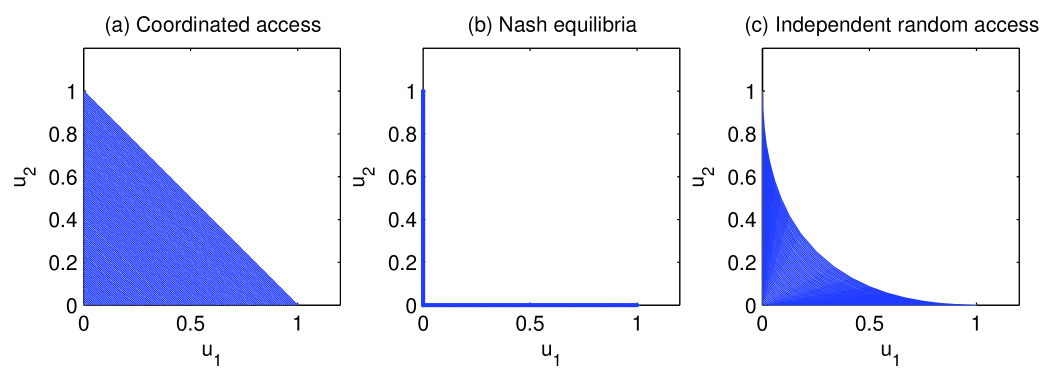
Figure 1: Payoff profiles with two homogeneous users with $k_{1}=k_{2}=1$. (a) The set of feasible payoffs when coordination between two users is possible. (b) The set of Nash equilibrium payoffs. (c) The set of feasible payoffs with independent transmission probabilities.

Figure 1 presents the payoff spaces of two homogeneous users with $k_{1}=k_{2}=1$. If coordination between the two users is possible, they can achieve any payoff profile in the dark area of Figure 1(a). For example, $(1/2,1/2)$ can be achieved by arranging user 1 to transmit only in odd-numbered slots and user 2 only in even-numbered slots. This kind of coordination can be supported through direct communications among the users or mediated communications. However, if such coordination is not possible and each user has to choose one transmission probability, Nash equilibria yield the payoff profiles in Figure 1(b). The set of feasible payoffs of the contention game is shown as the dark area of Figure 1(c). The set of Pareto-efficient payoff profiles is the frontier of that area. The lack of coordination makes the set of feasible payoffs smaller reducing the area of Figure 1(a) to that of Figure 1(c). Because the typical Nash equilibrium payoff is $(0,0)$, the next section develops a transformation of the contention game, and the set of equilibria of the resulting Stackelberg game is shown to expand to the entire area of Figure 1(c).

3 Stackelberg Contention Game

We introduce a network manager as a special kind of user in the contention game and call him user 0. As a user, the manager can access the channel with a certain transmission probability. However, the manager is different from the users in that he can choose his transmission probability depending on the transmission probabilities of the users. This ability of the manager enables him to act as the police. If the users access the channel excessively, the manager can intervene and punish them by choosing a high transmission probability, thus reducing the success rates of the users.

Formally, the strategy of the manager is an intervention function $g:P\rightarrow[0,1]$, which gives his transmission probability $p_{0}=g(\mathbf{p})$ when the strategy profile of the users is $\mathbf{p}$. $g(\mathbf{p})$ can be interpreted as the level of intervention or punishment by the manager when the users choose $\mathbf{p}$. Note that the level of intervention by the manager is the same for every user. We assume that the manager has a specific “target” strategy profile $\tilde{\mathbf{p}}$, that his transmission has no value to him (as well as to others), and that he is benevolent. One representation of his objective is the payoff function of the following form:

$$u_{0}(g,\mathbf{p})=\left\{\begin{array}[]{ll}1-g(\mathbf{p})&\textrm{if $\mathbf{p}=\tilde{\mathbf{p}}$},\\ 0&\textrm{otherwise}.\end{array}\right.$$ (6)

This payoff function means that the manager wants the users to operate at the target strategy profile $\tilde{\mathbf{p}}$ with the minimum level of intervention.

We call the transformed game the Stackelberg contention game because the manager chooses his strategy $g$ before the users make their decisions on the transmission probabilities. In this sense, the manager can be thought of as a Stackelberg leader and the users as followers. The specific timing of the Stackelberg contention game can be outlined as follows:

1. The network manager determines his intervention function.

2. Knowing the intervention function of the manager, the users choose their transmission probabilities simultaneously.

3. Observing the strategy profile of the users, the manager determines the level of intervention using his intervention function.

4. The transmission probabilities of the manager and the users determine their payoffs.

Timing 1 happens before the session starts. Timing 2 occurs at the beginning of the session whereas timing 3 occurs when the manager knows the transmission probabilities of all the users. Therefore, there is a time lag between the time when the session begins and when the manager starts to intervene. Payoffs can be calculated as the probability of successful transmission averaged over the entire session, multiplied by valuation. If the interval between timing 2 and timing 3 is short relative to the duration of the session, the payoff of user $i$ can be approximated as the payoff during the intervention using the following payoff function:

$$u_{i}(g,\mathbf{p})=k_{i}p_{i}(1-g(\mathbf{p}))\prod_{j\neq i}(1-p_{j}).$$ (7)

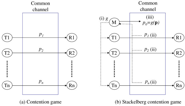
Figure 2: Schematic illustration of (a) the contention game and (b) the Stackelberg contention game. (i),(ii), and (iii) represent the order of moves in the Stackelberg contention game, and the dotted arrows represent the flows of information required for the Stackelberg contention game.

The transformation of the contention game into the Stackelberg contention game is schematically shown in Figure 2. The figure shows that the main role of the manager is to set the intervention rule and to implement it. The users still behave non-cooperatively maximizing their payoffs, and the intervention of the manager affects their selfish behavior even though the manager does neither directly control their behavior nor continuously communicate with the users to convey coordination or price signals.

In the Stackelberg routing game of [10], the strategy spaces of the manager and a user coincide. If that is the case in the Stackelberg contention game, i.e., if the manager chooses a single transmission probability before the users choose theirs, then this intervention only makes the channel lossy but it does not provide incentives for users not to choose the maximum possible transmission probability. Hence, in order to provide an incentive to choose a smaller transmission probability, the manager needs to vary his transmission probability depending on the transmission probabilities of the users.

A Stackelberg game is analyzed using a backward induction argument. The leader predicts the Nash equilibrium behavior of the followers given his strategy and chooses the best strategy for him. The same argument can be applied to the Stackelberg contention game. Once the manager decides his strategy $g$ and commits to implement his transmission probability according to $g$, the rest of the Stackelberg contention game (timing 2–4) can be viewed as a non-cooperative game played by the users. Given the intervention function $g$, the payoff function of user $i$ can be written as

$$\tilde{u}_{i}(\mathbf{p};g)=k_{i}p_{i}(1-g(\mathbf{p}))\prod_{j\neq i}(1-p_{j}).$$ (8)

In essence, the role of the manager is to change the non-cooperative game that the users play from the contention game $\Gamma$ to a new game $\Gamma_{g}=\langle N,(P_{i}),(\tilde{u}_{i}(\cdot;g))\rangle$, which we call the contention game with intervention $g$. Understanding the non-cooperative behavior of the users given the intervention function $g$, the manager will choose $g$ that maximizes his payoff.

We now define an equilibrium concept for the Stackelberg contention game.

Definition 1

An intervention function of the manager $g$ and a profile of the transmission probabilities of the users $\hat{\mathbf{p}}=(\hat{p}_{1},\ldots,\hat{p}_{n})$ constitutes a Stackelberg equilibrium if (i) $\hat{\mathbf{p}}$ is a Nash equilibrium of the contention game with intervention $g$ and (ii) $\hat{\textbf{p}}=\tilde{\textbf{p}}$ and $g(\hat{\mathbf{p}})=0$.

Combining (i) and (ii), an equivalent definition is that ($g,\tilde{\mathbf{p}})$ is a Stackelberg equilibrium if $\tilde{\mathbf{p}}$ is a Nash equilibrium of $\Gamma_{g}$ and $g(\tilde{\mathbf{p}})=0$. Condition (i) says that once the manager chooses his strategy, the users will play a Nash equilibrium strategy profile in the resulting game, and condition (ii) says that expecting the Nash equilibrium strategy profile of the users, the manager chooses his strategy that achieves his objective.

3.1 Stackelberg Equilibrium with TRD-based Intervention

As we have mentioned earlier, the manager can choose only one level of intervention that affects the users equally. A question that arises is which strategy profile the manager can implement as a Stackelberg equilibrium with one level of intervention for every user. We answer this question constructively. We propose a specific form of an intervention function with which the manager can attain any strategy profile $\tilde{\mathbf{p}}$ with $0<\tilde{p}_{i}<1$ for all $i$. The basic idea of this result is that because the strategy of the manager is not a single intervention level but a function whose value depends on the strategies of the users, he can discriminate the users by reacting differently to their transmission probabilities in choosing the level of intervention. Therefore, even though the realized level of intervention is the same for every user, the manager can induce the users to choose different transmission probabilities.

To construct such an intervention function, we first define the total relative deviation (TRD) of $\mathbf{p}$ from $\tilde{\mathbf{p}}$ by

$$h(\mathbf{p})=\sum_{i=1}^{n}\frac{p_{i}-\tilde{p}_{i}}{\tilde{p}_{i}}=\frac{p_{1}}{\tilde{p}_{1}}+\cdots+\frac{p_{n}}{\tilde{p}_{n}}-n.$$ (9)

Since $g$ determines the transmission probability of the manager, its range should lie in $[0,1]$. To satisfy this constraint, we define the TRD-based intervention function by

$$g^{*}(\mathbf{p})=\left[h(\mathbf{p})\right]_{0}^{1}$$ (10)

where the operator $[x]_{a}^{b}=\min\{\max\{x,a\},b\}$ is used to obtain the “trimmed” value of TRD between 0 and 1.

The TRD-based intervention can be interpreted in the following way. The manager sets the target at $\tilde{\mathbf{p}}$. As long as the users choose small transmission probabilities so that the TRD of $\mathbf{p}$ from $\tilde{\mathbf{p}}$ does not exceed zero, the manager does not intervene. If it is larger than zero, the manager will respond to a one-unit increase in $p_{i}$ by increasing $p_{0}$ by $\frac{1}{\tilde{p}_{i}}$ units until the TRD reaches 1. The manager determines the degree of punishment based on the target transmission probability profile. If he wants a user to transmit with a low probability, then his punishment against its deviation is strong.

Proposition 2

$(g^{*},\tilde{\mathbf{p}})$ constitutes a Stackelberg equilibrium.

Proof: We need to check two things. First, $\tilde{\mathbf{p}}$ is a Nash Equilibrium of $\Gamma_{g^{*}}$. Second, $g^{*}(\tilde{\mathbf{p}})=0$. It is straightforward to confirm the second. To show the first, the payoff function of user $i$ given others’ strategies $\tilde{\mathbf{p}}_{-i}$ is

$$\tilde{u}_{i}(p_{i},\tilde{\mathbf{p}}_{-i};g^{*}) = k_{i}p_{i}\left(1-g^{*}(p_{i},\tilde{\mathbf{p}}_{-i})\right)\prod_{j\neq i}(1-\tilde{p}_{j})$$ (11)

$$= \left\{\begin{array}[]{ll}0&\textrm{if $p_{i}>2\tilde{p}_{i}$},\\ k_{i}p_{i}\left(2-\frac{p_{i}}{\tilde{p}_{i}}\right)\prod_{j\neq i}(1-\tilde{p}_{j})&\textrm{if $\tilde{p}_{i}\leq p_{i}\leq 2\tilde{p}_{i}$},\\ k_{i}p_{i}\prod_{j\neq i}(1-\tilde{p}_{j})&\textrm{if $p_{i}<\tilde{p}_{i}$}.\end{array}\right.$$ (15)

It can be seen from the above expression that $\tilde{u}_{i}(p_{i},\tilde{\mathbf{p}}_{-i};g^{*})$ is increasing on $p_{i}<\tilde{p}_{i}$, reaches a peak at $p_{i}=\tilde{p}_{i}$, is decreasing on $\tilde{p}_{i}<p_{i}<2\tilde{p}_{i}$, and then stays at 0 on $p_{i}\geq 2\tilde{p}_{i}$. Therefore, user $i$’s best response to $\tilde{\mathbf{p}}_{-i}$ is $\tilde{p}_{i}$ for all $i$, and thus $\tilde{\mathbf{p}}$ constitutes a Nash Equilibrium of the contention game with TRD-based intervention, $\Gamma_{g^{*}}$.  

Corollary 1

Any feasible payoff profile $\mathbf{u}\in\mathcal{U}$ of the contention game with $u_{i}>0$ for all $i\in N$ can be achieved by a Stackelberg equilibrium.

Corollary 1 resembles the Folk theorem of repeated games [4] in that it claims that any feasible outcome can be attained as an equilibrium. Incentives not to deviate from a certain operating point are provided by the manager’s intervention in the Stackelberg contention game, while in a repeated game players do not deviate since a deviation is followed by punishment from other players.

3.2 Nash Equilibria of the Contention Game with TRD-based Intervention

In Proposition 2, we have seen that $\tilde{\mathbf{p}}$ is a Nash equilibrium of the contention game with TRD-based intervention. However, if other Nash equilibria exist, the outcome may be different from the one that the manager intends. In fact, any strategy profile $\mathbf{p}$ with $p_{i}=1$ for at least one $i$ is still a Nash equilibrium of $\Gamma_{g^{*}}$. The following proposition characterizes the set of Nash equilibria of $\Gamma_{g^{*}}$ that are different from those of $\Gamma$.

Proposition 3

Consider a strategy profile $\hat{\mathbf{p}}$ with $\hat{p}_{i}<1$ for all $i\in N$. $\hat{\mathbf{p}}$ is a Nash equilibrium of the contention game with TRD-based intervention if and only if either

$$(i)\quad\hat{\mathbf{p}}=\tilde{\mathbf{p}}$$ (16)

or

$$(ii)\quad\sum_{j\neq i}\frac{\hat{p}_{j}-\tilde{p}_{j}}{\tilde{p}_{j}}\geq 2\textrm{ for all $i=1,\ldots,n$}.$$ (17)

Proof: See Appendix A.  

Transforming $\Gamma$ to $\Gamma_{g^{*}}$ does not eliminate the Nash equilibria of the contention game. Rather, the set of Nash equilibria expands to include two classes of new equilibria. The first Nash equilibrium of Proposition 3 is the one that the manager intends the users to play. The second class of Nash equilibria are those in which the sum of relative deviations of other users is already too large that no matter how small transmission probability user $i$ chooses, the level of intervention stays the same at 1.

Since $\tilde{\mathbf{p}}$ is chosen to satisfy $0<\tilde{p}_{i}<1$ for all $i$ and $g^{*}$ satisfies $g^{*}(\tilde{\mathbf{p}})=0$, it follows that $\tilde{u}_{i}(\tilde{\mathbf{p}})>0$ for all $i$. For the second class of Nash equilibria in Proposition 3, $\tilde{u}_{i}(\hat{\mathbf{p}})=0$ for all $i$ because $g^{*}(\hat{\mathbf{p}})=1$. Therefore, the payoff profile of the second class of Nash equilibria is Pareto dominated by that of the intended Nash equilibrium in that the intended Nash equilibrium yields a higher payoff for every user compared to the second class of Nash equilibria.

The same conclusion holds for Nash equilibria with more than one user with transmission probability 1 because every user gets zero payoff. Finally, the remaining Nash equilibria are those with exactly one user with transmission probability 1. Suppose that $p_{i}=1$. Then the highest payoff for user $i$ is achieved when $p_{j}=0$ for all $j\neq i$. Denoting this strategy profile by $\mathbf{e}_{i}$, the payoff profile of $\mathbf{e}_{i}$ is Pareto dominated by that of $\tilde{\mathbf{p}}$ if $1-g^{*}(\mathbf{e}_{i})=1+n-\frac{1}{\tilde{p}_{i}}<\tilde{p}_{i}\prod_{j\neq i}(1-\tilde{p}_{j})$.

3.3 Reaching the Stackelberg Equilibrium

We have seen that there are multiple Nash equilibria of the contention game with TRD-based intervention and that the Nash equilibrium $\tilde{\mathbf{p}}$ in general yields higher payoffs to the users than other Nash equilibria. If the users are aware of the welfare properties of different Nash equilibria, they will tend to select $\tilde{\mathbf{p}}$.

Suppose that the users play the second class of Nash equilibria in Proposition 3 for some reason. If the Stackelberg contention game is played repeatedly and the users anticipate that the strategy profile of the other users will be the same as that of the last period, then it can be shown that under certain conditions there is a sequence of intervention functions convergent to $g^{*}$ that the manager can employ to have the users reach the intended Nash equilibrium $\tilde{\mathbf{p}}$, thus approaching the Stackelberg equilibrium.

Proposition 4

Suppose that at $t=0$ the manager chooses the intervention function $g^{*}$ and that the users play a Nash equilibrium $\hat{\mathbf{p}}^{0}$ of the second class.

Without loss of generality, the users are enumerated so that the following holds:

$$\frac{\hat{p}_{1}^{0}}{\tilde{p}_{1}}\leq\frac{\hat{p}_{2}^{0}}{\tilde{p}_{2}}\leq\ldots\leq\frac{\hat{p}_{n-1}^{0}}{\tilde{p}_{n-1}}\leq\frac{\hat{p}_{n}^{0}}{\tilde{p}_{n}}.$$ (18)

Suppose further that for each $i$, either $\frac{\hat{p}_{n}^{0}}{\tilde{p}_{n}}-\frac{\hat{p}_{i}^{0}}{\tilde{p}_{i}}<2$ or $\frac{\hat{p}_{i}^{0}}{\tilde{p}_{i}}\leq 1$ holds.

At $t\geq 1$; Define

$$c^{t}=\sum_{j\neq n}\frac{\hat{p}_{j}^{t-1}}{\tilde{p}_{j}}+1.$$ (19)

Assume that the manager employs the intervention function $g^{t}(\mathbf{p})=[h^{t}(\mathbf{p})]_{0}^{1}$ where

$$h^{t}(\mathbf{p})=\frac{p_{1}}{\tilde{p}_{1}}+\cdots+\frac{p_{n}}{\tilde{p}_{n}}-c^{t}$$ (20)

and that user $i$ chooses $\hat{p}_{i}^{t}$ as a best response to $\hat{\mathbf{p}}_{-i}^{t-1}$ given $g^{t}$.

Then $\lim_{t\rightarrow\infty}\hat{p}_{i}^{t}=\tilde{p}_{i}$ for all $i=1,\ldots,n$ and $\lim_{t\rightarrow\infty}c^{t}=n$.

Proof: See Appendix B.  

The reason that no user has an incentive to deviate from the second class of Nash equilibria is that since others use high transmission probabilities, the TRD is over 1 no matter what transmission probability a user chooses. Since the punishment level is always 1, a reduction of the transmission probability by a user is not rewarded by a decreased level of intervention. If the relative deviations of $p_{i}$ from $\tilde{p}_{i}$ are not too disperse, the manager can successively adjust down the effective range of punishment so that he can react to the changes in the strategies of the users. Proposition 4 shows that this procedure succeeds to have the strategy profile of the users converge to the intended Nash equilibrium.

4 Target Selection Criteria of the Manager

So far we have assumed that the manager has a target strategy profile $\tilde{\mathbf{p}}$ and examined whether he can find an intervention function that implements it as a Stackelberg equilibrium. This section discusses selection criteria that the manager can use to choose the target strategy profile. To address this issue, we rely on cooperative game theory because a reasonable choice of the manager should have a close relationship to the likely outcome of bargaining among the users if bargaining were possible for them [4]. The absence of communication opportunities among the users prevents them from engaging in bargaining or from directly coordinating with each other.

4.1 Nash Bargaining Solution

The pair $(F,\mathbf{v})$ is an n-person bargaining problem where $F$ is a closed and convex subset of $\mathbb{R}^{n}$, representing the set of feasible payoff allocations and $\mathbf{v}=(v_{1},\ldots,v_{n})$ is the disagreement payoff allocation. Suppose that there exists $\mathbf{y}\in F$ such that $y_{i}>v_{i}$ for every $i$.

Definition 2

$\mathbf{x}$ is the Nash bargaining solution for an n-person bargaining problem $(F,\mathbf{v})$ if it is the unique Pareto efficient vector that solves

$$\max_{\mathbf{x}\in F,\mathbf{x}\geq\mathbf{v}}\prod_{i=1}^{n}(x_{i}-v_{i}).$$ (21)

Consider the contention game $\Gamma$. $(\mathcal{U},\mathbf{0})$ can be regarded as an $n$-person bargaining problem where $\mathcal{U}$ is defined in (3) and $\mathbf{0}$ is the disagreement point. The vector $\mathbf{0}$ is the natural disagreement point because it is a Nash equilibrium payoff as well as the minimax value for each user. The only departure from the standard theory is that the set of feasible payoffs $\mathcal{U}$ is not convex. However, we can carry the definition of the Nash bargaining solution to our setting as in [15].

Since the manager knows the structure of the contention game, he can calculate the Nash bargaining solution $\mathbf{u}$ for $(\mathcal{U},\mathbf{0})$ and find the strategy profile $\tilde{\mathbf{p}}$ that yields $\mathbf{u}$. Then the manager can implement $\tilde{\mathbf{p}}$ by choosing $g^{*}$ based on $\tilde{\mathbf{p}}$. Notice that the presence of the manager does not decrease the payoffs of the users because $g^{*}(\tilde{\mathbf{p}})$ = 0. The Nash bargaining solution for $(\mathcal{U},\mathbf{0})$ has the following simple form.

Proposition 5

$\frac{(n-1)^{n-1}}{n^{n}}(k_{1},\ldots,k_{n})$ is the Nash bargaining solution for $(\mathcal{U},\mathbf{0})$, and it is attained by $p_{i}=\frac{1}{n}$ for all $i=1,\ldots,n$.

Proof: The maximand in the definition of the Nash bargaining solution can be written as

$$\max_{\mathbf{u}\in\mathcal{U},\mathbf{u}\geq\mathbf{0}}\prod_{i=1}^{n}u_{i}.$$ (22)

Since any $\mathbf{u}\in\mathcal{U}$ satisfies $\mathbf{u}\geq\mathbf{0}$, the above problem can be expressed in terms of $\mathbf{p}$:

$$\max_{\mathbf{p}\in P}\left(\prod_{i=1}^{n}k_{i}\right)\prod_{i=1}^{n}p_{i}(1-p_{i})^{n-1}.$$ (23)

The logarithm of the objective function is strictly concave in $\mathbf{p}$, and the first-order optimality condition gives $p_{i}=\frac{1}{n}$ for all $i=1,\ldots,n$.  

The Nash bargaining solution for $(\mathcal{U},\mathbf{0})$ treats every user equally in that it specifies the same transmission probability for every user. Therefore, the manager does not need to know the vector of the values of transmission $\mathbf{k}=(k_{1},\ldots,k_{n})$ to implement the Nash bargaining solution. The Nash bargaining solution coincides with the Kalai-Smorodinsky solution [16] because the maximum payoff for user $i$ is $k_{i}$ and the Nash bargaining solution is the unique efficient payoff profile in which each user receives a payoff proportional to its maximum feasible payoff.

If the manager wants to treat the users with discrimination, he can use the generalized Nash product

$$\prod_{i=1}^{n}(x_{i}-v_{i})^{\omega_{i}}$$ (24)

as the maximand to find a nonsymmetric Nash bargaining solution, where $\omega_{i}>0$ represents the weight for user $i$. One example of the weights is the valuation of the users. The nonsymmetric Nash bargaining solution for $(\mathcal{U},\mathbf{0})$ can be shown to be achieved by $p_{i}=\frac{\omega_{i}}{\sum_{i}\omega_{i}}$ for all $i$ using the similar method to the proof of Proposition 5.

4.2 Coalition-Proof Strategy Profile

If some of the users can communicate and collude effectively, the network manager may want to choose a strategy profile which is self-enforcing even in the existence of coalitions. Since we define a user as a transmitter-receiver pair, a collusion may occur when a single transmitter sends packets to several destinations and controls the transmission probabilities of several users.

Given the set of users $N=\{1,\ldots,n\}$, a coalition is any nonempty subset $S$ of $N$. Let $\mathbf{p}_{S}$ be the strategy profile of the users in $S$.

Definition 3

$\tilde{\mathbf{p}}$ is coalition-proof with respect to a coalition $S$ in a non-cooperative game $\langle N,[0,1]^{N},(u_{i})\rangle$ if there does not exist $\mathbf{p}_{S}\in[0,1]^{S}$ such that $u_{i}(\mathbf{p}_{S},\tilde{\mathbf{p}}_{-S})\geq u_{i}(\tilde{\mathbf{p}})$ for all $i\in S$ and $u_{i}(\mathbf{p}_{S},\tilde{\mathbf{p}}_{-S})>u_{i}(\tilde{\mathbf{p}})$ for at least one user $i\in S$.

By definition, $\tilde{\mathbf{p}}$ is coalition-proof with respect to the grand coalition $S=N$ if and only if $\mathbf{u}(\tilde{\mathbf{p}})=({u}_{1}(\tilde{\mathbf{p}}),\ldots,{u}_{n}(\tilde{\mathbf{p}}))$ is Pareto efficient. If $\tilde{\mathbf{p}}$ is a Nash equilibrium, then it is coalition-proof with respect to any one-person “coalition.” The non-cooperative game of our interest is the contention game with TRD-based intervention $g^{*}$.

Proposition 6

$\tilde{\mathbf{p}}$ is coalition-proof with respect to a two-person coalition $S=\{i,j\}$ in the contention game with TRD-based intervention $g^{*}$ if and only if $\tilde{p}_{i}+\tilde{p}_{j}\leq 1$.

Proof: See Appendix C.  

The proof of Proposition 6 shows that if $\tilde{p}_{i}+\tilde{p}_{j}>1$ then users $i$ and $j$ can jointly reduce their transmission probabilities to increase their payoffs at the same time. For example, suppose that users 1 and 2 are controlled by the same transmitter and that the manager selects the target $\tilde{\mathbf{p}}$ with $\tilde{p}_{1}=0.3$ and $\tilde{p}_{2}=0.8$. Then $\tilde{u}_{1}(\tilde{\mathbf{p}})=0.06\,k_{1}\prod_{j\neq 1,2}(1-\tilde{p}_{j})$ and $\tilde{u}_{2}(\tilde{\mathbf{p}})=0.56\,k_{2}\prod_{j\neq 1,2}(1-\tilde{p}_{j})$. Suppose that the two users jointly deviate to $(p_{1},p_{2})=(0.25,0.75)$. Then the new payoffs are $\tilde{u}_{1}(p_{1},p_{2},\tilde{\mathbf{p}}_{N\setminus\{1,2\}})=0.0625\,k_{1}\prod_{j\neq 1,2}(1-\tilde{p}_{j})$ and $\tilde{u}_{2}(p_{1},p_{2},\tilde{\mathbf{p}}_{N\setminus\{1,2\}})=0.5625\,k_{2}\prod_{j\neq 1,2}(1-\tilde{p}_{j})$, which is strictly better for both users. A decrease in $p_{i}$ and $p_{j}$ at the same time also increases the payoffs of all the users not belonging to the coalition, which implies that a target $\tilde{\mathbf{p}}$ with $\tilde{p}_{i}+\tilde{p}_{j}>1$ is not Pareto efficient. This observation leads to the following corollary.

Corollary 2

If $\tilde{\mathbf{p}}$ is Pareto efficient in the contention game with TRD-based intervention $g^{*}$, then it is coalition-proof with respect to any two-person coalition.

In fact, we can generalize the above corollary and provide a stronger statement.

Proposition 7

$\tilde{\mathbf{p}}$ is Pareto efficient in the contention game with TRD-based intervention $g^{*}$ if and only if it is coalition-proof with respect to any coalition.

Proof: See Appendix D.  

5 Informational Requirement and Its Relaxation

We have introduced and analyzed the contention game and the Stackelberg contention game with TRD-based intervention. In this section we discuss what the players of each game need to know in order to play the corresponding equilibrium.

5.1 Contention Game and Nash Equilibrium

In a general non-cooperative game, each user needs to know, or predict correctly, the strategy profile of others in order to find its best response strategy. In the contention game with the payoff function $u_{i}(\mathbf{p})=k_{i}p_{i}\prod_{j\neq i}(1-p_{j})$, it suffices for user $i$ to know the sign of $\prod_{j\neq i}(1-p_{j})$, i.e., whether it is positive or zero, to calculate its best response. On the other hand, $p_{i}=1$ is a weakly dominant strategy for any user $i$, which means setting $p_{i}=1$ is weakly better no matter what strategies other users choose. Hence, the Nash equilibrium $\mathbf{p}=(1,\ldots,1)$ does not require any knowledge on others’ strategies.

5.2 Stackelberg Contention Game with TRD-based Intervention and Stackelberg Equilibrium

Considering the timing of the Stackelberg contention game outlined in Section 3, we can list the following requirements on the manager and the users for the Stackelberg equilibrium to be played.

Requirement M. Once the users choose the transmission probabilities, the manager observes the strategy profile of the users.

The manager needs to decide the level of intervention as a function of the transmission probabilities of the users. If the manager can distinguish the access of each user and have sufficiently many observations to determine the transmission probability of each user, then this requirement will be satisfied. If the manager can observe the channel state (idle, success, collision) and identify the users of successfully transmitted packets, he can estimate the transmission probability of each user in the following way. First, he can obtain an estimate of $\prod_{i\in N}(1-p_{i})$ by calculating the frequency of idle slots, called $q_{idle}$. Second, he can obtain an estimate of $p_{i}\prod_{j\neq i}(1-p_{j})$ by calculating the frequency of slots in which user $i$ succeeds to transmit its packet, called $q_{i}$. Finally, an estimate of $p_{i}$ can be obtained by solving $\frac{p_{i}}{1-p_{i}}=\frac{q_{i}}{q_{idle}}$ for $p_{i}$.

Requirement U. User $i$ knows $g^{*}$ (and thus $\tilde{\mathbf{p}}$) and $\mathbf{p}_{-i}$ when it chooses its transmission probability.

Requirement U is sufficient for the Nash equilibrium of the contention game with TRD-based intervention to be played by the users. User $i$ can find its best response strategy by maximizing $\tilde{u}_{i}$ given $g^{*}$ and $\mathbf{p}_{-i}$. In fact, a weaker requirement is compatible with the Nash equilibrium of the contention game with TRD-based intervention. Suppose that user $i$ knows the form of intervention function $g^{*}$ and the value of $\tilde{p}_{i}$, and observes the intervention level $p_{0}$. $\tilde{\mathbf{p}}$ embedded in the TRD-based intervention function $g^{*}$ can be thought of as a recommended strategy profile by the manager (thus the communication from the manager to the users occurs indirectly through the function $g^{*}$). Even though user $i$ does not know the recommended strategies to other users, i.e., the values of $\tilde{p}_{j}$, $j\neq i$, it knows its recommended transmission probability. From the form of the intervention function, user $i$ can derive that it is of its best interest to follow the recommendation as long as all the other users follow their recommended strategies. Observing $p_{0}=0$ confirms its belief that other users play the recommended strategies, and it has no reason to deviate.

The users can acquire knowledge on the intervention function $g^{*}$ through one of three ways: (i) known protocol, (ii) announcement, and (iii) learning. The first method is effective in the case where a certain network manager operates in a certain channel (for example, a frequency band). The community of users will know the protocol (or intervention function) used by the manager. This method does not require any information exchange between the manager and the users. Neither teaching of the manager nor learning of the users is necessary. However, there is inflexibility in choosing an intervention function, and the manager cannot change his target strategy profile frequently. Nevertheless, this is the method most often used in current wireless networks, where users appertain to a predetermined class of known and homogeneous protocols.

The second method allows the manager to make the users know $g^{*}$ directly, which includes information on the target $\tilde{\mathbf{p}}$. The manager will execute his intervention according to the announced intervention function because the Stackelberg equilibrium $(g^{*},\tilde{\mathbf{p}})$ achieves his objective. However, it requires explicit message delivery from the manager to the users, which is sometimes costly or may even be impossible in practice.

Finally, if the Stackelberg contention game is played repeatedly with the same intervention function, the users may be able to recover the form of the intervention function chosen by the manager based on their observations on $(p_{0},{\mathbf{p}})$, for example, using learning techniques developed in [17, 18, 19]. However, this process may take long and the users may not be able to collect enough data to find out the true functional form if there is limited experimentation of the users.

Remark. If users are obedient, the manager can use centralized control by communicating $\tilde{p}_{i}$ to user $i$. Additional communication and estimation overhead required for the Stackelberg equilibrium can be considered as a cost incurred to deal with the selfish behavior of users, or to provide incentives for users to follow $\tilde{\mathbf{p}}$.

5.3 Limited Observability of the Manager

The construction of the TRD-based intervention function assumes that the manager can observe or estimate the transmission probabilities of the users correctly. In real applications, the manager may not be able to observe the exact choice made by each user. We consider several scenarios under which the manager has limited observability and examine how the TRD-based intervention function can be modified in those scenarios.

5.3.1 Quantized Observation

Let $\mathcal{I}=\{I_{0},I_{1},\ldots,I_{m}\}$ be a set of intervals which partition $[0,1]$. We assume that each interval contains its right end point. For simplicity, we will consider intervals of the same length. That is, $\mathcal{I}=\left\{\{0\},\left(0,\frac{1}{m}\right],\left(\frac{1}{m},\frac{2}{m}\right],\ldots,\left(\frac{m-1}{m},1\right]\right\}$, and we call $I_{0}=\{0\}$ and $I_{r}=\left(\frac{r-1}{m},\frac{r}{m}\right]$ for all $r=1,\ldots,m$.

Suppose that the manager only observes which interval in $\mathcal{I}$ each $p_{i}$ belongs to. In other words, the manager observes $r_{i}$ instead of $p_{i}$ such that $p_{i}\in I_{r_{i}}$. In this case, the level of intervention is calculated based on $\mathbf{r}=(r_{1},\ldots,r_{n})$ rather than $\mathbf{p}$. It means that given $\mathbf{p}_{-i}$, $p_{0}$ would be the same for any $p_{i},p^{\prime}_{i}$ if $p_{i}$ and $p^{\prime}_{i}$ belong to the same $I_{r}$. Since any $p_{i}\in\left(\frac{r-1}{m},\frac{r}{m}\right)$ is weakly dominated by $p_{i}=\frac{r}{m}$, the users will choose their transmission probabilities at the right end points of the intervals in $\mathcal{I}$. This in turn will affect the choice of a target by the manager. The manager will be restricted to choose $\tilde{\mathbf{p}}$ such that $\tilde{p}_{i}\in\left\{\frac{1}{m},\ldots,\frac{m-1}{m}\right\}$ for all $i\in N$. Then the manager can implement $\tilde{\mathbf{p}}$ with the intervention function $g(\mathbf{r})=g^{*}(\mathbf{p})$, where $p_{i}$ is set equal to $\frac{r_{i}}{m}$. In summary, the quantized observation on $\mathbf{p}$ restricts the choice of $\tilde{\mathbf{p}}$ by the manager from $(0,1)^{N}$ to $\left\{\frac{1}{m},\ldots,\frac{m-1}{m}\right\}^{N}$.

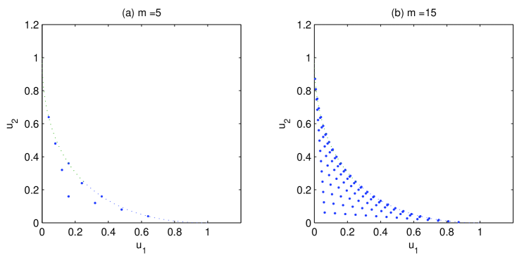
Figure 3: Payoffs that can be achieved by the manager with quantized observation. (a) $m=5$. (b) $m=15$.

Figure 3 shows the payoff profiles that can be achieved by the manager with quantized observation. When the number of intervals is moderately large, the manager has many options near or on the Pareto efficiency boundary.

5.3.2 Noisy Observation

We modify the Stackelberg contention game to analyze the case where the manager observes noisy signals of the transmission probabilities of the users. Let $P_{i}=[\epsilon,1-\epsilon]$ be the strategy space of user $i$, where $\epsilon$ is a small positive number. We assume that the users can observe the strategy profile $\mathbf{p}$, but the manager observes a noisy signal of $\mathbf{p}$. The manager observes $p_{i}^{o}$ instead of $p_{i}$ where $p_{i}^{o}$ is uniformly distributed on $[p_{i}-\epsilon,p_{i}+\epsilon]$, independently over $i\in N$. Suppose that the manager chooses a target $\tilde{\mathbf{p}}$ such that $\tilde{p}_{i}\in[2\epsilon,1-2\epsilon]$. The expected payoff of user $i$ when the manager uses an intervention function $g$ is

$$E[\tilde{u}_{i}(\mathbf{p};g)|\mathbf{p}]=k_{i}p_{i}\prod_{j\neq i}(1-p_{j})\left(1-E[g(\mathbf{p}^{o})|\mathbf{p}]\right).$$ (25)

Hence, the intervention function is effectively $E[g(\mathbf{p}^{o})|\mathbf{p}]$ instead of $g(\mathbf{p})$ when the manager observes $\mathbf{p}^{o}$. If $\hat{\mathbf{p}}$ is a Nash equilibrium of the contention game with intervention $g$ when $\mathbf{p}$ is perfectly observable to the manager and $E[g(\mathbf{p}^{o})|\mathbf{p}]=g(\mathbf{p})$ for all $\mathbf{p}$ such that $\max_{i\in N}|p_{i}-\hat{p}_{i}|\leq\epsilon$, then $\hat{\mathbf{p}}$ will still be a Nash equilibrium of the contention game with intervention $g$ when the manager observes a noisy signal of the strategy profile of the users.

Consider the TRD-based intervention function $g^{*}$. Since $g^{*}(\mathbf{p})\geq 0$ for all $\mathbf{p}\in P$ and $h(\mathbf{p}^{o})>0$ with a positive probability when $\mathbf{p}=\tilde{\mathbf{p}}$, $E[g^{*}(\mathbf{p}^{o})|\tilde{\mathbf{p}}]>0$ whereas $g^{*}(\tilde{\mathbf{p}})=0$. Since $g^{*}$ is kinked at $\tilde{\mathbf{p}}$, the noise in $\mathbf{p}^{o}$ will distort the incentives of the users to choose $\tilde{\mathbf{p}}$.

The manager can implement his target $\tilde{\mathbf{p}}$ at the expense of intervention with a positive probability. If the manager adopts the following intervention function

$$g(\mathbf{p})=\sum_{i\in N}\frac{\frac{1}{1+\epsilon q}p_{i}-\tilde{p}_{i}}{\tilde{p}_{i}}+\frac{(n+1)\epsilon q}{1+\epsilon q},$$ (26)

where $q=\sum_{i\in N}\frac{1}{\tilde{p}_{i}}$, then $\tilde{\mathbf{p}}$ is a Nash equilibrium of the contention game with intervention $g$, but the average level of intervention at $\tilde{\mathbf{p}}$ is

$$E[g(\mathbf{p}^{o})|\tilde{\mathbf{p}}]=g(\tilde{\mathbf{p}})=\frac{\epsilon q}{1+\epsilon q}>0,$$ (27)

which can be thought of as the efficiency loss due to the noise in observations.

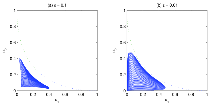
Figure 4: Payoffs that can be achieved by the manager with noisy observation. (a) $\epsilon=0.1$. (b) $\epsilon=0.01$.

Figure 4 illustrates the set of payoff profiles that can be achieved with the intervention function given by (26). As the size of the noise gets smaller, the set expands to approach the Pareto efficiency boundary.

5.3.3 Observation on the Aggregate Probability

We consider the case where the manager can observe only the frequency of the slots that are not accessed by any user. If the users transmit their packets according to $\mathbf{p}$, then the manager observes only the aggregate probability $\prod_{i\in N}(1-p_{i})$. In this scenario, the intervention function that the manager chooses has to be a function of $\prod_{i\in N}(1-p_{i})$, and this implies that the manager cannot discriminate among the users.

The TRD-based intervention function $g^{*}$ allows the manager to use different reactions to each user’s deviation. In the effective region where the TRD is between 0 and 1, one unit increase in $p_{i}$ results in $\frac{1}{\tilde{p}_{i}}$ units increase in $p_{0}$. However, this kind of discrimination through the structure of the intervention function is impossible when the manager cannot observe individual transmission probabilities.

This limitation forces the manager to treat the users equally, and the target has to be chosen such that $\tilde{p}_{i}=\tilde{p}$ for all $i\in N$. If the manager uses the following intervention function,

$$g(\mathbf{p})=\left[\frac{1}{\tilde{p}(1-\tilde{p})^{n-1}}\left((1-\tilde{p})^{n}-\prod_{i\in N}(1-p_{i})\right)\right]_{0}^{1}$$ (28)

then he can implement $\tilde{\mathbf{p}}=(\tilde{p},\ldots,\tilde{p})$ with $g(\tilde{\mathbf{p}})=0$ as a Stackelberg equilibrium. Hence, if the manager only observes the aggregate probability, this prevents him from setting the target transmission probabilities differently across users.

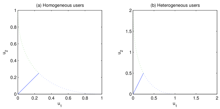
Figure 5: Payoffs that can be achieved by the manager who observes only the aggregate probability. (a) Homogeneous users with $k_{1}=k_{2}=1$. (b) Heterogeneous users with $k_{1}=1$ and $k_{2}=2$.

Figure 5 shows the payoff profiles achieved with symmetric strategy profiles, which can be implemented by the manager who observes the aggregate probability.

5.4 Limited Observability of the Users and Conjectural Equilibrium

We now relax Requirement U and assume that user $i$ can observe only the aggregate probability $(1-p_{0})\prod_{j\neq i}(1-p_{j})$. Even though the users do not know the exact form of the intervention function of the manager, they are aware of the dependence of $p_{0}$ on their transmission probabilities and try to model this dependence based on their observations $(p_{i},(1-p_{0})\prod_{j\neq i}(1-p_{j}))$. Specifically, user $i$ builds a conjecture function $f_{i}:[0,1]\rightarrow[0,1]$, which means that user $i$ conjectures that the value of $(1-p_{0})\prod_{j\neq i}(1-p_{j})$ will be $f_{i}(p_{i})$ if he chooses $p_{i}$. The equilibrium concept appropriate in this context is conjectural equilibrium first introduced by Hahn [20].

Definition 4

A strategy profile $\hat{\mathbf{p}}$ and a profile of conjectures $(f_{1},\ldots,f_{n})$ constitutes a conjectural equilibrium of the contention game with intervention $g$ if

$$k_{i}\hat{p}_{i}\,f_{i}(\hat{p}_{i})\geq k_{i}p_{i}\,f_{i}(p_{i})\quad\textrm{for all }p_{i}\in P_{i}$$ (29)

and

$$f_{i}(\hat{p}_{i})=(1-g(\hat{\mathbf{p}}))\prod_{j\neq i}(1-\hat{p}_{j})$$ (30)

for all $i\in N$.

The first condition states that $\hat{p}_{i}$ is optimal given user $i$’s conjecture $f_{i}$, and the second condition says that its conjecture is consistent with its observation. It can be seen from this definition that the conjectural equilibrium is a generalization of Nash equilibrium in that any Nash equilibrium is a conjectural equilibrium with every user holding the correct conjecture given others’ strategies. On the other hand, it is quite general in some cases, and in the game we consider, for any strategy profile $\hat{\mathbf{p}}\in P$, there exists a conjecture profile $(f_{1},\ldots,f_{n})$ that constitutes a conjectural equilibrium. For example, we can set $f_{i}(p_{i})=(1-g(\hat{\mathbf{p}}))\prod_{j\neq i}(1-\hat{p}_{j})$ if $p_{i}=\hat{p}_{i}$ and 0 otherwise.

Since the TRD-based intervention function $g^{*}$ is linear in each $p_{i}$, it is natural for the users to adopt a conjecture function of the linear form. Let us assume that conjecture functions are of the following trimmed linear form:

$$f_{i}(p_{i})=\left[a_{i}-b_{i}p_{i}\right]_{0}^{1}$$ (31)

for some $a_{i},b_{i}>0$.

We say that a conjecture function $f_{i}$ is linearly consistent at $\hat{\mathbf{p}}$ if it is locally correct up to the first derivative at $\hat{\mathbf{p}}$, i.e., $f_{i}(\hat{p}_{i})=(1-g(\hat{\mathbf{p}}))\prod_{j\neq i}(1-\hat{p}_{j})$ and $f^{\prime}_{i}(\hat{p}_{i})=-\frac{\partial g(\hat{\mathbf{p}})}{\partial p_{i}}\prod_{j\neq i}(1-\hat{p}_{j})$. Since the TRD-based intervention function $g^{*}$ is linear in each $p_{i}$, the conjecture function $f_{i}^{*}(p_{i})\triangleq g^{*}(p_{i},\tilde{\mathbf{p}}_{-i})$ is linearly consistent at $\tilde{\mathbf{p}}$, and $\tilde{\mathbf{p}}$ and $(f_{1}^{*},\ldots,f_{n}^{*})$ constitutes a conjectural equilibrium. Therefore, as long as the users use linearly consistent conjectures, limited observability of the users does not affect the final outcome. To build linearly consistent conjectures, however, the users need to experiment and collect data using local deviations from the equilibrium point in a repeated play of the Stackelberg contention game. A loss in performance may result during this learning phase.

6 Illustrative Results

6.1 Homogeneous Users

We assume that the users are homogeneous with $k_{i}=1$ for all $i\in N$. Given a transmission probability profile ${\mathbf{p}}$, the system utilization ratio can be defined as the probability of successful transmission in a given slot

$$\tau(\mathbf{p})=\sum_{i\in N}p_{i}\prod_{j\neq i}(1-p_{j}).$$ (32)

Note that the maximum system utilization ratio is 1, which occurs when only one user transmits with probability 1 while others never transmit. Table 1 shows the individual payoffs and the system utilization ratios for the number of users 3, 10, and 100 when the manager implements the target at the symmetric efficient strategy profile $\tilde{\mathbf{p}}=(\frac{1}{n},\ldots,\frac{1}{n})$.

$n$	Individual Payoff	System Utilization Ratio
3	0.14815	0.44444
10	0.03874	0.38742
100	0.00370	0.36973

Table 1. Individual payoffs and system utilization ratios with homogeneous users

We can see that packets are transmitted in approximately 37% of the slots with a large number of users even if there is no explicit coordination among the users. The system utilization of our model converges to $1/e\approx 36.8\%$ as $n$ goes to infinity, which coincides with the maximal throughput of a slotted Aloha system with Poisson arrivals and an infinite number of users [21]. But in our model users maintain their selfish behavior, and we do not use any feedback information on the channel state.

6.2 Heterogeneous Users

We now consider users with difference valuations. Specifically, we assume that $k_{i}=i$ for $i=1,\ldots,n$. We will consider three targets: $\tilde{\mathbf{p}}^{1}=(1,\ldots,n)/\sum_{i=1}^{n}i$, $\tilde{\mathbf{p}}^{2}=(\frac{1}{n},\ldots,\frac{1}{n})$, and $\tilde{\mathbf{p}}^{3}$ with which $\tilde{u}_{i}(\tilde{\mathbf{p}}^{3};g^{*})=\tilde{u}_{j}(\tilde{\mathbf{p}}^{3};g^{*})$ for all $i,j$. $\tilde{\mathbf{p}}^{1}$ assigns a higher transmission probability to a user with a higher valuation. $\tilde{\mathbf{p}}^{2}$ treats all the users equally regardless of their valuations. $\tilde{\mathbf{p}}^{3}$ is egalitarian in that it yields the same individual payoff to every user, which implies that a user with a low valuation is assigned a higher transmission probability.

		Average	Aggregate	Standard	System	Nash	Generalized
Target	$n$	Individual	Payoff	Deviation of	Utilization	Product	Nash
		Payoff		Payoffs	Ratio		Product
	3	0.38889	1.16667	0.32710	0.47222	1.28601e-2	2.48073e-3
$\tilde{\mathbf{p}}^{1}$	10	0.28048	2.80481	0.24643	0.39384	3.40193e-9	4.57497e-30
	100	0.24855	24.85466	0.22189	0.37034	2.12632e-98	$\approx$ 0
	3	0.29630	0.88889	0.12096	0.44444	1.95092e-2	1.14183e-3
$\tilde{\mathbf{p}}^{2}$	10	0.21308	2.13081	0.11127	0.38742	2.76432e-8	4.83117e-34
	100	0.18671	18.67135	0.10673	0.36973	5.73364e-86	$\approx$ 0
	3	0.25133	0.75400	0	0.46078	1.58765e-2	2.52064e-4
$\tilde{\mathbf{p}}^{3}$	10	0.13753	1.37533	0	0.40283	2.42148e-9	4.09682e-48
	100	0.07303	7.30337	0	0.37885	2.25070e-114	$\approx$ 0

Table 2. Average individual payoffs, aggregate payoffs, standard deviations of individual payoffs, system utilization ratios, Nash products, and generalized Nash products with heterogeneous users

Table 2 shows that a tradeoff between efficiency (measured by the sum of payoffs) and equity exists when users are heterogeneous. A higher aggregate payoff is achieved when users with high valuations are given priority. At the same time, it limits access by users with low valuations, which increases variations in individual payoffs. Also, the results in Table 2 are consistent with that $\tilde{\mathbf{p}}^{2}$ is a Nash bargaining solution and that $\tilde{\mathbf{p}}^{1}$ is a nonsymmetric Nash bargaining solution with weights equal to valuations.

7 Conclusion

We have analyzed the problem of multiple users who share a common communication channel. Using the game theory framework, we have shown that selfish behavior is likely to lead to a network collapse. However, full system utilization requires coordination among users using explicit message exchanges, which may be impractical given the distributed nature of wireless networks. To achieve a better performance without coordination schemes, users need to sustain cooperation. We provide incentives for selfish users to limit their access to the channel by introducing an intervention function of the network manager. With TRD-based intervention functions, the manager can implement any outcome of the contention game as a Stackelberg equilibrium. We have discussed the amount of information required for implementation, and how the various kinds of relaxations of the requirements affect the outcome of the Stackelberg contention game.

Our approach of using an intervention function to improve network performance can be applied to other situations in wireless communications. Potential applications of the idea include sustaining cooperation in multi-hop networks and limiting the attack of adversary users. An intervention function may be designed to serve as a coordination device in addition to providing selfish users with incentives to cooperate. Finally, designing a protocol that enables users to play the role of the manager in a distributed manner will be critical to ensure that our approach can be adopted in completely decentralized communication scenarios, where no manager is present.

Appendix A Proof of Proposition 3

Recall $h(\mathbf{p})=\frac{p_{1}}{\tilde{p}_{1}}+\cdots+\frac{p_{n}}{\tilde{p}_{n}}-n$ used to define $g^{*}(\mathbf{p})$. We examine whether a strategy profile $\hat{\mathbf{p}}$ with $\hat{p}_{i}<1$ for all $i\in N$ constitutes a Nash equilibrium of $\Gamma_{g^{*}}$ by considering four cases on the value of $h(\hat{\mathbf{p}})$.

Case 1. $h(\hat{\mathbf{p}})<0$.

Let $\epsilon=-h(\hat{\mathbf{p}})>0$. If user $i$ changes its transmission probability from $\hat{p}_{i}$ to $\hat{p}_{i}+\epsilon$, then its payoff increases because $p_{0}$ is still zero. Hence $\hat{\mathbf{p}}$ cannot be a Nash equilibrium if $h(\hat{\mathbf{p}})<0$.

Case 2. $h(\hat{\mathbf{p}})=0$.

Consider arbitrary user $i$. If it deviates to $p_{i}<\hat{p}_{i}$, $p_{0}$ is still zero and $\tilde{u}_{i}$ decreases. $\tilde{u}_{i}(p_{i},\hat{\mathbf{p}}_{-i})$ is differentiable and strictly concave on $p_{i}>\hat{p}_{i}$. Since $\frac{d\tilde{u}_{i}}{dp_{i}}=(k_{i}\prod_{j\neq i}(1-\hat{p}_{j}))(1+n-\sum_{j\neq i}\frac{\hat{p}_{j}}{\tilde{p}_{j}}-2\frac{p_{i}}{\tilde{p}_{i}})$, $k_{i}>0$ and $\hat{p}_{i}<1$ for all $i$,

$$sign\left(\frac{d\tilde{u}_{i}}{dp_{i}}\Bigg{|}_{p_{i}=\hat{p}_{i}}\right) = sign\left(1+n-\sum_{j\neq i}\frac{\hat{p}_{j}}{\tilde{p}_{j}}-2\frac{\hat{p}_{i}}{\tilde{p}_{i}}\right)$$ (33)

$$= sign\left(1+n-\sum_{j=1}^{n}\frac{\hat{p}_{j}}{\tilde{p}_{j}}-\frac{\hat{p}_{i}}{\tilde{p}_{i}}\right)$$ (34)

$$= sign\left(1-\frac{\hat{p}_{i}}{\tilde{p}_{i}}\right).$$ (35)

There is no gain for user $i$ from deviating to any $p_{i}>\hat{p}_{i}$ if and only if $\frac{d\tilde{u}_{i}}{dp_{i}}|_{p_{i}=\hat{p}_{i}}\leq 0$, which is equivalent to $\hat{p}_{i}\geq\tilde{p}_{i}$. For $\hat{\mathbf{p}}$ to be a Nash equilibrium, we need $\hat{p}_{i}\geq\tilde{p}_{i}$ for all $i=1,\ldots,n$. To satisfy $h(\hat{\mathbf{p}})=0$, all inequalities should be equalities. Hence, only $\hat{\mathbf{p}}=\tilde{\mathbf{p}}$ is a Nash equilibrium among $\hat{\mathbf{p}}$ such that $h(\hat{\mathbf{p}})=0$.

Case 3. $0<h(\hat{\mathbf{p}})<1$.

Since $\tilde{u}_{i}\geq 0$, there is no gain for user $i$ to deviate to $p_{i}$ such that $h(p_{i},\hat{\mathbf{p}}_{-i})\geq 1$. If there is a gain from deviation to $p_{i}$ such that $h(p_{i},\hat{\mathbf{p}}_{-i})<0$, then there is another profitable deviation $p^{\prime}_{i}$ such that $h(p^{\prime}_{i},\hat{\mathbf{p}}_{-i})=0$ by using the argument of Case 1. Therefore, we can restrict our attention to deviations $p_{i}$ that lead to $0\leq h(p_{i},\hat{\mathbf{p}}_{-i})<1$. At such a deviation by user $i$,

$$\tilde{u}_{i}(p_{i},\hat{\mathbf{p}}_{-i})=k_{i}\prod_{j\neq i}(1-\hat{p}_{j})p_{i}\left(1+n-\sum_{j\neq i}\frac{\hat{p}_{j}}{\tilde{p}_{j}}-\frac{p_{i}}{\tilde{p}_{i}}\right).$$ (36)

$\hat{p}_{i}$ is best response to $\hat{\mathbf{p}}_{-i}$ if and only if $\frac{d\tilde{u}_{i}}{dp_{i}}|_{p_{i}=\hat{p}_{i}}=0$. Using the first derivative given in Case 2, we obtain

$$\frac{\hat{p}_{i}}{\tilde{p}_{i}}=1+n-\sum_{j=1}^{n}\frac{\hat{p}_{j}}{\tilde{p}_{j}}=1-h(\hat{\mathbf{p}})<1.$$ (37)

For $\hat{\mathbf{p}}$ to be a Nash equilibrium, the above inequality should be satisfied for every $i$, which in turn implies

$$\sum_{i=1}^{n}\frac{\hat{p}_{i}}{\tilde{p}_{i}}<n,$$ (38)

and this contradicts to the initial assumption $h(\hat{\mathbf{p}})>0$. Therefore, there is no $\hat{\mathbf{p}}$ with $0<h(\hat{\mathbf{p}})<1$ that constitutes a Nash equilibrium.

Case 4. $h(\hat{\mathbf{p}})\geq 1$.

Since $\tilde{u}_{i}(\hat{\mathbf{p}})=0$ for every $i$, there is a profitable deviation of user $i$ only if there exists $p_{i}\in(0,\hat{p}_{i})$ such that $h(p_{i},\hat{\mathbf{p}}_{-i})<1$. Equivalently, if setting $p_{i}=0$ yields $h(p_{i},\hat{\mathbf{p}}_{-i})\geq 1$, then there is no profitable deviation of user $i$ from $\hat{p}_{i}$. Since

$$h(0,\hat{\mathbf{p}}_{-i})=\sum_{j\neq i}\frac{\hat{p}_{j}}{\tilde{p}_{j}}-n,$$ (39)

$\hat{p}$ with $h(\hat{\mathbf{p}})\geq 1$ is a Nash equilibrium if and only if

$$\sum_{j\neq i}\frac{\hat{p}_{j}}{\tilde{p}_{j}}-n\geq 1\textrm{ for all $i=1,\ldots,n$}.$$ (40)

Appendix B Proof of Proposition 4

Consider $t=1$. User $i$ chooses $\hat{p}_{i}^{1}$ to maximize

$$\tilde{u}_{i}^{1}(p_{i},\hat{\mathbf{p}}_{-i}^{0}) = k_{i}p_{i}\left(1-g^{1}(p_{i},\hat{\mathbf{p}}_{-i}^{0})\right)\prod_{j\neq i}(1-\hat{p}_{j}^{0})$$ (41)

$$= \left\{\begin{array}[]{ll}k_{i}\prod_{j\neq i}(1-\hat{p}_{j}^{0})p_{i}&\textrm{if $p_{i}<\tilde{p}_{i}\left(1-\frac{\hat{p}_{n}^{0}}{\tilde{p}_{n}}+\frac{\hat{p}_{i}^{0}}{\tilde{p}_{i}}\right)$},\\ k_{i}\prod_{j\neq i}(1-\hat{p}_{j}^{0})p_{i}\left(2-\frac{\hat{p}_{n}^{0}}{\tilde{p}_{n}}+\frac{\hat{p}_{i}^{0}}{\tilde{p}_{i}}-\frac{p_{i}}{\tilde{p}_{i}}\right)&\textrm{if $\tilde{p}_{i}\left(1-\frac{\hat{p}_{n}^{0}}{\tilde{p}_{n}}+\frac{\hat{p}_{i}^{0}}{\tilde{p}_{i}}\right)\leq p_{i}\leq\tilde{p}_{i}\left(2-\frac{\hat{p}_{n}^{0}}{\tilde{p}_{n}}+\frac{\hat{p}_{i}^{0}}{\tilde{p}_{i}}\right)$},\\ 0&\textrm{if $p_{i}>\tilde{p}_{i}\left(2-\frac{\hat{p}_{n}^{0}}{\tilde{p}_{n}}+\frac{\hat{p}_{i}^{0}}{\tilde{p}_{i}}\right)$}.\end{array}\right.$$ (45)

If $0\leq\frac{\hat{p}_{n}^{0}}{\tilde{p}_{n}}-\frac{\hat{p}_{i}^{0}}{\tilde{p}_{i}}<2$, the maximum is attained at $\hat{p}_{i}^{1}$ that satisfies

$$\frac{\hat{p}_{i}^{1}}{\tilde{p}_{i}}=1-\frac{1}{2}\left(\frac{\hat{p}_{n}^{0}}{\tilde{p}_{n}}-\frac{\hat{p}_{i}^{0}}{\tilde{p}_{i}}\right).$$ (46)

Notice that $\hat{p}_{n}^{1}=\tilde{p}_{n}$.

If $\frac{\hat{p}_{n}^{0}}{\tilde{p}_{n}}-\frac{\hat{p}_{i}^{0}}{\tilde{p}_{i}}\geq 2$, then $\tilde{u}_{i}^{1}(p_{i},\hat{\mathbf{p}}_{-i}^{0})=0$ for all $p_{i}\geq 0$. Since any $p_{i}$ is a best response in this case, we assume that $\hat{p}_{i}^{1}=\hat{p}_{i}^{0}$.

Consider $t=2$. First, consider user $i$ such that $\frac{\hat{p}_{n}^{0}}{\tilde{p}_{n}}-\frac{\hat{p}_{i}^{0}}{\tilde{p}_{i}}<2$. Since $\frac{\hat{p}_{n}^{1}}{\tilde{p}_{n}}-\frac{\hat{p}_{i}^{1}}{\tilde{p}_{i}}=\frac{1}{2}\left(\frac{\hat{p}_{n}^{0}}{\tilde{p}_{n}}-\frac{\hat{p}_{i}^{0}}{\tilde{p}_{i}}\right)$, $0\leq\frac{\hat{p}_{n}^{1}}{\tilde{p}_{n}}-\frac{\hat{p}_{i}^{1}}{\tilde{p}_{i}}<2$. Using an analogous argument, we get

$$\frac{\hat{p}_{i}^{2}}{\tilde{p}_{i}}=1-\frac{1}{2}\left(\frac{\hat{p}_{n}^{1}}{\tilde{p}_{n}}-\frac{\hat{p}_{i}^{1}}{\tilde{p}_{i}}\right)=1-\frac{1}{2^{2}}\left(\frac{\hat{p}_{n}^{0}}{\tilde{p}_{n}}-\frac{\hat{p}_{i}^{0}}{\tilde{p}_{i}}\right).$$ (47)

Next consider user $i$ such that $\frac{\hat{p}_{i}^{0}}{\tilde{p}_{i}}\leq 1$. Since $\frac{\hat{p}_{n}^{1}}{\tilde{p}_{n}}=1$, we again have $0\leq\frac{\hat{p}_{n}^{1}}{\tilde{p}_{n}}-\frac{\hat{p}_{i}^{1}}{\tilde{p}_{i}}<2$ and the best response is given by

$$\frac{\hat{p}_{i}^{2}}{\tilde{p}_{i}}=1-\frac{1}{2}\left(\frac{\hat{p}_{n}^{1}}{\tilde{p}_{n}}-\frac{\hat{p}_{i}^{1}}{\tilde{p}_{i}}\right)=1-\frac{1}{2}\left(\frac{\hat{p}_{n}^{1}}{\tilde{p}_{n}}-\frac{\hat{p}_{i}^{0}}{\tilde{p}_{i}}\right).$$ (48)

Considering a general $t\geq 2$, we get

$$\frac{\hat{p}_{i}^{t}}{\tilde{p}_{i}}=1-\frac{1}{2^{t}}\left(\frac{\hat{p}_{n}^{0}}{\tilde{p}_{n}}-\frac{\hat{p}_{i}^{0}}{\tilde{p}_{i}}\right)$$ (49)

for user $i$ such that $\frac{\hat{p}_{n}^{0}}{\tilde{p}_{n}}-\frac{\hat{p}_{i}^{0}}{\tilde{p}_{i}}<2$ and

$$\frac{\hat{p}_{i}^{t}}{\tilde{p}_{i}}=1-\frac{1}{2^{t-1}}\left(\frac{\hat{p}_{n}^{1}}{\tilde{p}_{n}}-\frac{\hat{p}_{i}^{0}}{\tilde{p}_{i}}\right)$$ (50)

for user $i$ such that $\frac{\hat{p}_{i}^{0}}{\tilde{p}_{i}}\leq 1$. Taking limits as $t\rightarrow\infty$, we obtain the conclusions of the proposition.

Appendix C Proof of Proposition 6

Suppose that the users in the coalition $S=\{i,j\}$ choose $(p_{i},p_{j})$ instead of $(\tilde{p}_{i},\tilde{p}_{j})$. Then

$$h(p_{i},p_{j},\tilde{\mathbf{p}}_{-S})=\frac{p_{i}}{\tilde{p}_{i}}+\frac{p_{j}}{\tilde{p}_{j}}+(n-2)-n=\frac{p_{i}}{\tilde{p}_{i}}+\frac{p_{j}}{\tilde{p}_{j}}-2,$$ (51)

and

$$\tilde{u}_{i}(p_{i},p_{j},\tilde{\mathbf{p}}_{-S})=k_{i}\prod_{k\notin S}(1-\tilde{p}_{k})p_{i}(1-p_{j})(1-g^{*}(p_{i},p_{j},\tilde{\mathbf{p}}_{-S})),$$ (52)

$$\tilde{u}_{j}(p_{i},p_{j},\tilde{\mathbf{p}}_{-S})=k_{j}\prod_{k\notin S}(1-\tilde{p}_{k})p_{j}(1-p_{i})(1-g^{*}(p_{i},p_{j},\tilde{\mathbf{p}}_{-S})).$$ (53)

Hence, $\tilde{\mathbf{p}}$ is coalition-proof with respect to $S$ if and only if there does not exist $(p_{i},p_{j})\in[0,1]^{2}$ such that

$$p_{i}(1-p_{j})(1-g^{*}(p_{i},p_{j},\tilde{\mathbf{p}}_{-S})) \geq \tilde{p}_{i}(1-\tilde{p}_{j}),$$ (54)

$$p_{j}(1-p_{i})(1-g^{*}(p_{i},p_{j},\tilde{\mathbf{p}}_{-S})) \geq \tilde{p}_{j}(1-\tilde{p}_{i})$$ (55)

with at least one inequality strict.

First, notice that setting $p_{i}=\tilde{p}_{i}$ and $p_{j}\neq\tilde{p}_{j}$ will violate one of the two inequalities. The inequality for user $i$ will not hold if $p_{j}>\tilde{p}_{j}$, and the one for user $j$ will not hold if $p_{j}<\tilde{p}_{j}$. Hence, both $p_{i}\neq\tilde{p}_{i}$ and $p_{j}\neq\tilde{p}_{j}$ are necessary to have both inequalities satisfied at the same time. We consider four possible cases.

Case 1. $p_{i}<\tilde{p}_{i}$ and $p_{j}>\tilde{p}_{j}$

Since $g^{*}(\cdot)\geq 0$, (54) is violated.

Case 2. $p_{i}>\tilde{p}_{i}$ and $p_{j}<\tilde{p}_{j}$

Equation (55) is violated.

Case 3. $p_{i}<\tilde{p}_{i}$ and $p_{j}<\tilde{p}_{j}$

Since $h(p_{i},p_{j},\tilde{\mathbf{p}}_{-S})<0$, $g^{*}(p_{i},p_{j},\tilde{\mathbf{p}}_{-S})=0$. Hence, (54) and (55) become

$$p_{i}(1-p_{j}) \geq \tilde{p}_{i}(1-\tilde{p}_{j}),$$ (56)

$$p_{j}(1-p_{i}) \geq \tilde{p}_{j}(1-\tilde{p}_{i}).$$ (57)

We consider the contour curves of $p_{i}(1-p_{j})$ and $p_{j}(1-p_{i})$ going through $(\tilde{p}_{i},\tilde{p}_{j})$ in the $(p_{i},p_{j})$-plane. The slope of the contour curve of $p_{i}(1-p_{j})$ at $(\tilde{p}_{i},\tilde{p}_{j})$ is $\frac{1-\tilde{p}_{j}}{\tilde{p}_{i}}$ and that of $p_{j}(1-p_{i})$ is $\frac{\tilde{p}_{j}}{1-\tilde{p}_{i}}$. There is no area of mutual improvement if and only if

$$\frac{1-\tilde{p}_{j}}{\tilde{p}_{i}}\geq\frac{\tilde{p}_{j}}{1-\tilde{p}_{i}},$$ (58)

which is equivalent to $\tilde{p}_{i}+\tilde{p}_{j}\leq 1$.

Case 4. $p_{i}>\tilde{p}_{i}$ and $p_{j}>\tilde{p}_{j}$

Since $h(p_{i},p_{j},\tilde{\mathbf{p}}_{-S})>0$, $g^{*}(p_{i},p_{j},\tilde{\mathbf{p}}_{-S})=h(p_{i},p_{j},\tilde{\mathbf{p}}_{-S})$ as long as $\frac{p_{i}}{\tilde{p}_{i}}+\frac{p_{j}}{\tilde{p}_{j}}\leq 3$. Hence, (54) and (55) become

$$p_{i}(1-p_{j})\left(3-\frac{p_{i}}{\tilde{p}_{i}}-\frac{p_{j}}{\tilde{p}_{j}}\right) \geq \tilde{p}_{i}(1-\tilde{p}_{j}),$$ (59)

$$p_{j}(1-p_{i})\left(3-\frac{p_{i}}{\tilde{p}_{i}}-\frac{p_{j}}{\tilde{p}_{j}}\right) \geq \tilde{p}_{j}(1-\tilde{p}_{i}).$$ (60)

The slope of the contour curve of $p_{i}(1-p_{j})\left(3-\frac{p_{i}}{\tilde{p}_{i}}-\frac{p_{j}}{\tilde{p}_{j}}\right)$ at $(\tilde{p}_{i},\tilde{p}_{j})$ is

$$\frac{(1-\tilde{p}_{j})\left(3-2\frac{\tilde{p}_{i}}{\tilde{p}_{i}}-\frac{\tilde{p}_{j}}{\tilde{p}_{j}}\right)}{\tilde{p}_{i}\left(3+\frac{1}{\tilde{p}_{j}}-\frac{\tilde{p}_{i}}{\tilde{p}_{i}}-2\frac{\tilde{p}_{j}}{\tilde{p}_{j}}\right)}=0,$$ (61)

and that of $p_{j}(1-p_{i})\left(3-\frac{p_{i}}{\tilde{p}_{i}}-\frac{p_{j}}{\tilde{p}_{j}}\right)$ is

$$\frac{\tilde{p}_{j}\left(3+\frac{1}{\tilde{p}_{i}}-2\frac{\tilde{p}_{i}}{\tilde{p}_{i}}-\frac{\tilde{p}_{j}}{\tilde{p}_{j}}\right)}{(1-\tilde{p}_{i})\left(3-\frac{\tilde{p}_{i}}{\tilde{p}_{i}}-2\frac{\tilde{p}_{j}}{\tilde{p}_{j}}\right)}=+\infty.$$ (62)

Therefore, there is no $(p_{i},p_{j})>(\tilde{p}_{i},\tilde{p}_{j})$ that satisfies (54) and (55) at the same time.

Appendix D Proof of Proposition 7

The “if” part is trivial because a strategy profile that is coalition-proof with respect to the grand coalition is Pareto efficient. To establish the “only if” part, we will prove that if for a given strategy profile there exists a coalition that can improve the payoffs of its members then its deviation will not hurt other users outside of the coalition, which shows that the original strategy profile is not Pareto efficient.

Consider a strategy profile $\tilde{\mathbf{p}}$ and a coalition $S\subset N$ that can improve upon $\tilde{\mathbf{p}}$ by deviating from $\tilde{\mathbf{p}}_{S}$ to $\mathbf{p}_{S}$. Let $p_{0}=g^{*}(\mathbf{p}_{S},\tilde{\mathbf{p}}_{-S})$ the transmission probability of the manager after the deviation by coalition $S$. Since choosing $\mathbf{p}_{S}$ instead of $\tilde{\mathbf{p}}_{S}$ yields higher payoffs to the members of $S$, we have

$$p_{i}(1-p_{0})\prod_{j\in S\setminus\{i\}}(1-p_{j})\geq\tilde{p}_{i}\prod_{j\in S\setminus\{i\}}(1-\tilde{p}_{j})$$ (63)

for all $i\in S$ with at least one inequality strict. We want to show that the members not in the coalition $S$ do not get lower payoffs as a result of the deviation by $S$, that is,

$$(1-p_{0})\prod_{j\in S}(1-p_{j})\geq\prod_{j\in S}(1-\tilde{p}_{j}).$$ (64)

Suppose $(1-p_{0})\prod_{j\in S}(1-p_{j})<\prod_{j\in S}(1-\tilde{p}_{j})$. We can see that $p_{0}<1$ and $0<p_{i}<1$ for all $i\in S$ because the right-hand side of (63) is strictly positive. Combining this inequality with (63) yields $p_{i}>\tilde{p}_{i}$ for all $i\in S$, which implies $p_{0}>0$.

We can write $p_{i}=\tilde{p}_{i}+\epsilon_{i}$ for some $\epsilon_{i}>0$ for $i\in S$. Then $p_{0}=g^{*}(\mathbf{p}_{S},\tilde{\mathbf{p}}_{-S})=\sum_{i\in S}\frac{\epsilon_{i}}{\tilde{p}_{i}}$. (63) can be rewritten as

$$\tilde{p}_{i}\prod_{j\in S\setminus\{i\}}(1-\tilde{p}_{j}) \leq (\tilde{p}_{i}+\epsilon_{i})(1-p_{0})\prod_{j\in S\setminus\{i\}}(1-\tilde{p}_{j}-\epsilon_{j})$$ (65)

$$< (\tilde{p}_{i}+\epsilon_{i})(1-p_{0})\prod_{j\in S\setminus\{i\}}(1-\tilde{p}_{j})$$ (66)

for all $i\in S$. Simplifying this gives

$$\frac{\epsilon_{i}}{\tilde{p}_{i}}>\frac{p_{0}}{1-p_{0}}$$ (67)

for all $i\in S$. Summing these inequalities up over $i\in S$, we get

$$p_{0}=\sum_{i\in S}\frac{\epsilon_{i}}{\tilde{p}_{i}}>|S|\frac{p_{0}}{1-p_{0}}$$ (68)

where $|S|$ is the number of the members in $S$. This inequality simplifies to $p_{0}<1-|S|\leq 0$, which is a contradiction.

References

- [1] J.-W. Lee, A. Tang, J. Huang, M. Chiang, and A. R. Calderbank, “Reverse-engineering MAC: a non-cooperative game model,” IEEE Journal on Selected Areas in Communications, vol. 25, no. 6, pp. 1135–1147, 2007.
- [2] G. Tan and J. Guttag, “The 802.11 MAC protocol leads to inefficient equilibria,” in Proceedings of the 24th Annual Joint Conference of the IEEE Computer and Communications Societies (INFOCOM 2005), vol. 1, pp. 1–11, Miami, FL, USA, March 2005.
- [3] R. T. Ma, V. Misra, and D. Rubenstein, “Modeling and analysis of generalized slotted-Aloha MAC protocols in cooperative, competitive and adversarial environments,” in Proceedings of the 26th IEEE International Conference on Distributed Computing Systems (ICDCS ’06), Lisboa, Portugal, July 2006.
- [4] R. Myerson, Game Theory: Analysis of Conflict, Harvard University Press, Cambridge, MA, USA, 1991.
- [5] E. Altman, N. Bonneau, and M. Debbah, “Correlated equilibrium in access control for wireless communications,” in Proceedings of NETWORKING 2006, pp. 173–183, Coimbra, Portugal, May 2006.
- [6] J. K. MacKie-Mason and H. R. Varian, “Pricing congestible network resources,” IEEE Journal on Selected Areas in Communications, vol. 13, no. 7, pp. 1141–1149, 1995.
- [7] Y. Jin and G. Kesidis, “A pricing strategy for an Aloha network of heterogeneous users with inelastic bandwidth requirements,” in Proceedings of the 39th Annual Conference on Information Sciences and Systems, Princeton, NJ, USA, March 2002.
- [8] D. Wang, C. Comaniciu, and U. Tureli, “A fair and efficient pricing strategy for slotted Aloha in MPR models,” in Proceedings of the 64th IEEE Vehicular Technology Conference, pp. 2474–2478, Montréal, Canada, September 2006.
- [9] R. Johari and J. N. Tsitsiklis, “Efficiency loss in a network resource allocation game,” Mathematics of Operations Research, vol. 29, no. 3, pp. 407–435, 2004.
- [10] Y. A. Korilis, A. A. Lazar, and A. Orda, “Achieving network optima using Stackelberg routing strategies,” IEEE/ACM Transactions on Networking, vol. 5, no. 1, pp. 161–173, 1997.
- [11] M. Bloem, T. Alpcan, and T. Başar, “A Stackelberg game for power control and channel allocation in cognitive radio networks,” in Proceedings of the 1st International Workshop on Game Theory in Communication Networks (GameComm2007), Nantes, France, October 2007.
- [12] L. Chen, T. Cui, S. H. Low, and J. C. Doyle, “ A game-theoretic model for medium access control,” in Proceedings of the 3rd International Wireless Internet Conference, Austin, TX, USA, October 2007.
- [13] L. Chen, S. H. Low, and J. C. Doyle, ”Contention control: a game-theoretic approach,” in Proceedings of the 46th IEEE Conference on Decision and Control, pp. 3428–3434, New Orleans, LA, USA, December 2007.
- [14] A. H. Mohsenian-Rad, J. Huang, M. Chiang, and V. W. S. Wong, “Utility-optimal random access without message passing,” IEEE Transactions on Wireless Communications, vol. 8, no. 3, pp. 1073–1079, 2009.
- [15] M. Ĉagalj, S. Ganeriwal, I. Aad, and J.-P. Hubaux, “On selfish behavior in CSMA/CA networks,” in Proceedings of the 24th Annual Joint Conference of the IEEE Computer and Communications Societies (INFOCOM 2005), vol. 4, pp. 2513–2524, Miami, FL, USA, March 2005.
- [16] E. Kalai and M. Smorodinsky, “Other solutions to Nash’s bargaining problem,” Econometrica, vol. 45, no. 3, pp. 513–518, 1975.
- [17] M. P. Wellman and J. Hu, “Conjectural equilibrium in multiagent learning,” Machine Learning, vol. 33, pp. 179–200, 1998.
- [18] J. Hu and M. P. Wellman, “Online learning about other agents in a dynamic multiagent system,” in Proceedings of the 2nd International Conference on Autonomous Agents, pp. 239–246, Minneapolis, MN, USA, May 1998.
- [19] Y. Vorobeychik, M. P. Wellman and S. Singh, “Learning payoff functions in infinite games,” Machine Learning, vol. 67, pp. 145–168, 2007.
- [20] F. H. Hahn, “Exercises in conjectural equilibria,” Scandinavian Journal of Economics, vol. 79, no. 2, pp. 210–226, 1977.
- [21] D. Bertsekas and R. Gallager, Data Networks, Prentice Hall, Englewood Cliffs, NJ, USA, 1987.