Methods for the Study of Transverse Momentum Differential Correlations
Abstract
We introduce and compare three differential correlation functions for the study of transverse momentum correlation in and collisions. These consist of inclusive, event-wise and a differential version of the correlation measure introduced by Gavin Gavin for experimental study of the viscosity per unit entropy of the matter produced in collisions. We study the quantitative difference between the three observables on the basis of PYTHIA simulations of collisions and collisions consisting of an arbitrary superposition of collision events at 200 GeV. We observe that inclusive and event-wise correlation functions are remarkably identical to each other where as the observable differs from the two. We study the robustness and efficiency dependencies of these observables based on truncated Taylor expansions in efficiency in collisions and on the basis of Monte Carlo simulation using an adhoc detector efficiency parameterization. We find that all the three observables are essentially independent of detector efficiency. We additionally study the scaling of the correlation measures and find all the observables exhibit an approximate dependence of the number of participants (N) in collisions. Finally, we study the impact of flow-like anisotropy on the inclusive correlation function and find flow imparts azimuthal modulations similar to those observed with two-particle densities.
pacs:
24.60.Ky, 25.75.-q, 25.75.Nq, 25.75.GzI Introduction
Measurements of two- and multi-particle correlations have proven a powerful tool to study heavy ion collision dynamics. In particular, measurements of two-particle correlations in the form of two-particle densities as a function of the particle pseudorapidities and azimuthal angles in collisions have revealed new correlation features not found in interactions. Specifically, azimuthal two-particle correlations in central collisions exhibit novel “away-side” structures, commonly referred as the away-side dip, and a near-side structure called the “ridge”. First measurements of the “dip” and “ridge” were reported on the basis of inclusive charged particle correlations dipRidge . More recently, measurements were extended to include identified charged and neutral particles, studies of correlations in various momentum ranges and system size dependencies SoftRidge . Measurements of event-by-event fluctuation observables such as net charge and transverse momentum provide complementary information. Studies of net charge and transverse momentum fluctuations show that while the magnitude of the fluctuations observed in collisions differs from that observed in collisions (after proper scaling to account for the number of collision participants), no dramatic suppression of the net charge fluctuations is observed that might signal the formation of a Quark Gluon Plasma (QGP) Pruneau03 ; Pruneau08 . Similarly, only small differences are observed in the magnitude of dynamical fluctuations in collisions relative to those observed in interactions after scaling by the number of participants and the particle average . The measured dynamical fluctuations in thus do not provide evidence for the strongly enhanced fluctuations expected for nuclear matter near the tri-critical point StarPtPt . In contrast, however, the width of the charge balance function exhibits a significant reduction from peripheral to central collisions that is consistent with the predictions of delayed hadronization when a QGP is formed StarBalanceFct . The reduction of the balance function measured as a function of pseudorapidity may, however, result from radial flow, resonance decays, or other effects. It is thus important to seek additional observables to obtain a better understanding of the collision dynamics.
In this work, we consider measurements of differential transverse momentum two-particle correlations as a function of the relative pseudorapidity and azimuthal angles of measured particles. A certain latitude exists in the calculation of such correlation functions. Indeed, as for integral correlations StarPtPt ; Adams:2004gp , one can use both inclusive and event-wise definitions. One can also consider dynamical fluctuations as the difference between measured fluctuations and statistical fluctuations i.e. those expected for a purely Poisson system. Extensions of fluctuation variables GazdzickiMrowczynski and Trainor are also possible. In this work, we study three differential observables namely, inclusive and event-wise correlation functions and a differential version of the measure , used by Gavin GavinAbdelAziz07 ; Gavin08 to estimate the viscosity per unit entropy of the matter formed in collisions. The observable definitions and notation used in this work are presented in Sect. II. In Sect. III, we focus on the definition of these observables for the study of transverse momentum correlations between two particles as functions of the relative pseudorapidity, and azimuthal angles of the particles. The goal of these observables is essentially to measure the covariance of two particle momenta by averaging the product of the differences between these momenta and the mean momentum. Given their different definition, one expects, in practice, they should measure different numerical values. The quantitative differences between these observables are assessed in Sect. IV on the basis of generic arguments and PYTHIA simulations. Section V presents predictions based on the event generator PYTHIA Pythia . Sect. VI discusses the dependence of these observables on the number of participants in collisions. Elliptic flow effects on the magnitude and azimuthal dependence of these observables is discussed in Sect. VII. The experimental robustness of these observables is studied in Sect. VIII. This work is summarized in Sect. IX.
II Notation and Definitions
We consider measurements of one- and two-particle production cross-sections. We are specifically interested in the measurements of two-particle correlations. Let and represent arbitrary observables for two particles, i=1, 2. These observables may be the momenta, azimuthal angle, pseudorapidity etc., of the particles. Let and be one- and two-particle densities, respectively, defined as functions of these observables.
| (1) | |||||
| (2) |
Discussions in this paper are limited to two-particle correlations but can be straightforwardly extended to higher order multi-particle correlations. For simplicity, and illustrative purposes, assume the particles are indistinguishable. Integrals of the above densities over the space spanned by observables () yield the number of particles and pairs of particles, respectively, in the domain of integration.
| (3) |
| (4) |
where N is the average number of particles produced in the region of acceptance of interest.
Experimentally, the number of particles in a given acceptance fluctuates event-by-event owing to the stochastic nature of the production processes. The one- and two-particle densities may then be viewed as an average of the number of particles taken over all measured events. We label events with an index , where is the number of events in the data sample. One measures the number of particles, at a given location in a bin of width for each event . The one- particle and two- particle densities are then obtained by averaging over the event ensemble, i.e. the total number of events .
| (5) |
| (6) |
where represents the event-ensemble average of .
In this work we describe measurements of fluctuations and a differential correlation observable. This requires measurements of covariances where and is the mean value of x, which is a function of coordinates and . Such a function of and corresponds to a average taken with respect to the two-particle density given by Eq. 2. To denote such averages we use the notation , where g(x) is some function of the coordinates , and n = 1,2 signifies the one- or two- particle density, respectively. For example, the average value of x as a function of y, as defined below, denoted , is defined and calculated as:
| (7) |
where is the value of for particle at position in an event . similarly the two-particle covariance , a function of and is denoted and is defined and calculated as:
| (8) |
The number of pairs in an event is given by the product of the number of particles, , in bins of width at positions and . However, the number of pairs is reduced to for identical bins (indistinguishable particles).
The above expressions correspond to what is commonly referred to as inclusive averages. An alternative averaging method is also available which corresponds to event-wise average. event-wise averages of and are herein noted as and , respectively. They are calculated as follows:
| (9) | |||||
| (10) |
where
| (11) |
For integral correlations where the above averages are taken over a single wide bin, the above expression (Eq.10) reduces to fluctuation variables reported in recent works Voloshin05 ; StarPtPt .
Gavin suggested recently Gavin08 that the width of transverse momentum fluctuation distributions measured as a function of pseudorapidity may be used to estimate the viscosity of the matter formed in collisions studied at RHIC and LHC.
Here we consider a differential version of the correlation , and write
| (12) |
A number of other observables have been used recently to carry out measurements of fluctuations and are well documented in the literature. The quantity , defined in GazdzickiMrowczynski , was used by CERN experiments NA49 and CERES to measure transverse momentum fluctuations in Pb + Pb collisions. The quantity was used by STAR to measure fluctuations in Au + Au collisions Voloshin:2005qj . There is an approximate equivalence between these different integral observables as shown in VoloshinPRD60_1999
III Transverse Momentum Differential Correlations
In this section, we focus our discussion on integral and differential transverse momentum correlations. Integral correlations, , may in principle provide an estimate of event-by-event temperature fluctuations which, in turn, may provide means to determine the heat capacity of the medium formed in collisions Stodolsky95 ; KorusMrowczynski2001 ; Stephanov0110077 . Additionally, one can also use the measure , defined in Sect. 2, to study the transverse momentum correlations SoftRidge ; GavinAbdelAziz07 ; Gavin08 . We argue that a differential version of all the observables, as defined in the previous section, may provide an equivalent or even better way to estimate the medium viscosity. However, calculation of viscosity using these observables is not presented in this work. Clearly, differential correlation functions provide more information than integrals over a wide range of pseudorapidity. Therefore they may enable a deeper understanding of the collision dynamics at play in collisions. As a specific example one notes the discovery of the “ridge” in two-particle (density) correlations measured in collisions. It is thus interesting to consider differential transverse momentum correlations as a function of differences in particle pseudorapidity and azimuthal angles (denoted as and , respectively).
To simplify the notation, we use rather than the “usual” to denote transverse momentum. We define the transverse momentum correlations of interest by substituting for in Eq. 7 through Eq. 12, and include a dependency on the particles’ pseudorapidity, , and azimuthal angle, . The inclusive momentum correlation function is defined as
| (13) |
and calculated using the following expression:
| (14) |
where one applies the conditions and . is the number of particles detected in a given event at pseudorapidity and laboratory angle . represents the transverse momentum of particle from event . is the inclusive average particle transverse momentum at and .
| (15) |
We include dependencies of the average transverse momentum, , on the laboratory angles and to account for possible instrumental effects. The mean is independent of azimuthal angles and for unpolarized beams. The detector acceptance and particle detection efficiency may, however, vary with these angles and must thus be accounted for in practice.
The event-wise transverse momentum correlation is calculated as follows.
| (16) |
and uses the event-wise average
| (17) |
Similarly can be written as:
| (18) |
IV Comparison of Differential Correlation Observables
The inclusive and event-wise differential correlation observables, as well as the correlation measure , are designed to study the magnitude of correlation in terms of some specific kinematic variable x, where x may be, e.g., the particle transverse momentum or pseudorapidity. The three observables represent averages of the difference between the x value of each particle relative to the mean value of x. The three observables, however, employ distinct averaging methods and in general lead to different numerical results. None of these averaging methods can be considered “superior” in any sense. However, due to practical or technical reasons, studies of correlations are typically reported using one type of averaging only. Still other averaging methods were advocated and used in recent works Phenix ; Voloshin2002 ; CERES ; NA49 ; STAR2005 ; Adams:2004gp . Experimenters, therefore, have a choice of observables and have in fact reported data using many of these averaging methods. The different methods used by several experiments produce results that cannot be trivially compared from one experiment to another. The issue is compounded by the fact that these observables have different dependencies on the detection efficiency and acceptance. It is therefore of considerable interest to determine how different are the numerical values produced by these different averaging methods and correlation observable definitions. One can also find out whether values measured by an experiment using one observable can be meaningfully compared to those of different experiments or measurements using other observables.
We first note that if particle production follows perfect Poisson statistics, the correlation functions defined in the previous section are, by construction, null. The inclusive, event-wise and observables are thus trivially identical in the Poisson fluctuation limit. However, due to energy, momentum and quantum number conservation, particle production in general is a non-poissonian stochastic phenomenon, i.e. the correlation functions are non-zero. Below we investigate how different they can be in practice.
In order to investigate the differences between the inclusive, event-wise and observables, we consider a decomposition of the one- and two-particle densities using fixed multiplicity densities. We write
| (19) |
| (20) |
where expresses the probability of having a multiplicity ‘m’ in the measured and bin. Similarly, corresponds to the probability of finding and particles simultaneously in bins () and (), respectively. and are the single and pair densities for a fixed value of multiplicity (). Note that in the above expressions we have included a dependency on only for brevity ( dependencies can obviously also be included). By construction, one has
| (21) |
| (22) |
Integration restricted to particle momenta yields the pseudorapidity densities:
| (23) | |||||
| (24) |
The averages of the transverse momentum, , and at fixed multiplicity ‘m’ are
| (25) | |||||
| (26) |
Given the multiplicity (, ) is (are) fixed, the above expressions are valid and identical for the inclusive and event-wise averaging methods. Thus for fixed multiplicity densities the inclusive and event-wise averages are truely comparable for analyzing actual densities such as occur in and collisions. Based on Eqs. 13, 14, 19 & 20, the inclusive and means are expressed as follows in terms of the fixed multiplicity densities:
| (27) | |||||
| (28) | |||||
The mean and the fluctuations within a single wide range of pseudorapidity are given by
| (29) | |||||
| (30) |
The event-wise mean and the are calculated in a similar fashion.
| (31) | |||||
| (32) | |||||
For a wide bin of integrated pseudorapidity this becomes
| (33) | |||||
| (34) |
Lastly, expressed in terms of fixed multiplicity densities is calculated as follows:
| (35) | |||||
Though the inclusive, event-wise and quantities are manifestly different, they exhibit interesting similarities. We first consider the difference between the inclusive mean, , and the event-wise mean, , for large integrated ranges of pseudorapidity. Assuming is roughly constant over the multiplicity range of interest, one finds
| (36) | |||
| (37) |
i.e. the inclusive and event-wise mean should be approximately equal. This approximation is most likely valid for large domains of integration in pseudorapidity and in central collisions, which yield large multiplicities. In this case, it is reasonable to expect that varies slowly with m and one thus expects the difference between the two observables to be the smallest. On the other hand for small domains of integration or small multiplicity is more likely to depend on m and consequently one expects the two average methods to exhibit larger numerical differences.
The inclusive, event-wise and two-particle correlations can be approximated in the same manner. One finds for integral, or wide bin averages:
| (39) | |||||
| (40) | |||||
where we have again assumed both and vary slowly with ‘m’. One finds that in the limit where and are independent of , the inclusive and event-wise observables are strictly equal. In practice, the equality is only approximate given the average particle momentum is a function of event multiplicity. Additionally, given that for large values of , and relatively narrow range of multiplicity values, the ratio is, typically near unity. Therefore, one concludes that is also roughly equal to for large multiplicities. The above arguments and approximate equalities hold for integral correlations (or fluctuations) but are weaker for differential correlations. Indeed, in the case of differential correlations, the number of particle in a given pseudorapidity bin is quite small. The approximations used in Eqs. 21 & 22 are thus likely to be inappropriate and one should expect significant differences between the three observables; particularly between the inclusive average and . Any comparison of results from experiments reported on the basis of different observables is thus at best qualitative. We explore these differences further in Sect. V on the basis of PYTHIA simulations.
V Model Predictions
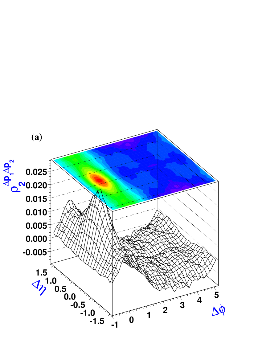
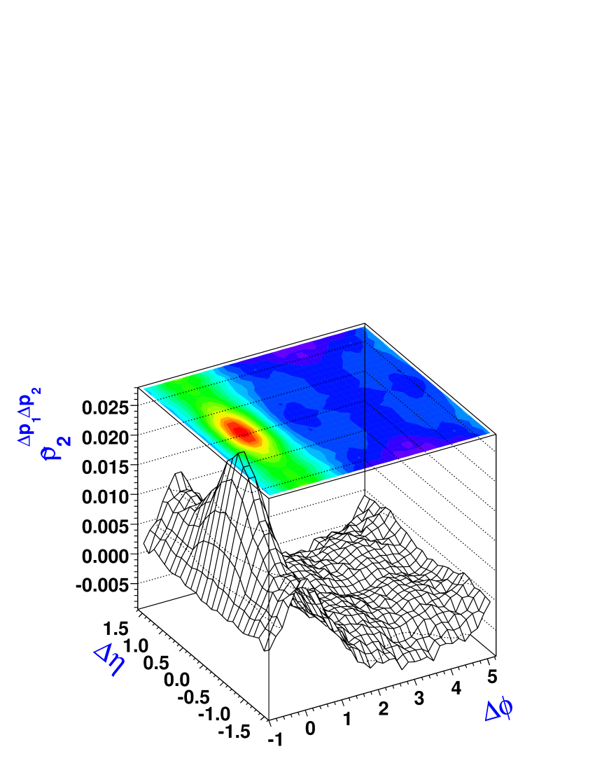
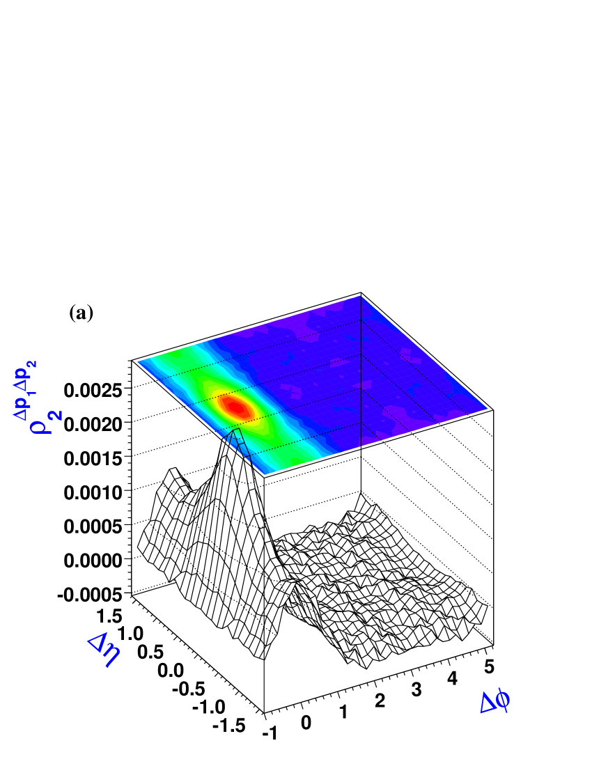
We use PYTHIA (version 6.22) Pythia to simulate collisions at GeV and carry out calculations of transverse momentum correlations based on the observables introduced in Sect III. Five million minimum bias PYTHIA events were integrated to produce plots shown in the following. Figures 1(a-c) show the inclusive, , event-wise, and correlation functions, respectively, for particles in the pseudorapidity range and transverse momentum range GeV/c. The two-particle correlations are plotted as a function of the particles’ relative pseudorapidity, , and azimuthal angles, , using 31 and 36 bins, respectively.
The three correlation functions show qualitative similarities: all three observables exhibit a peak structure near (near side) and a ridge-like structure at (away side) which extends over the full range. These shapes are qualitatively similar to that of density correlations predicted by PYTHIA Pruneau07 . While the inclusive and event-wise correlation functions are identical to each other with a difference of only 0.2% (statistical errors are of the order of 0.001), the observable exhibits characteristically different strength and shape. In contrast to inclusive and event-wise observables, the away side ridge-like structure has larger magnitude than the near side. One also finds that has a strength five times larger than the other two observables. A detailed study of reveals that the shape is largely determined by density correlations, . In contrast to inclusive and event-wise measures, which are designed to minimize the number density contribution is sensitive to the variation of the of the particles as well as the number density. As a result we conclude that the differences between the three observables stem from their specific definitions and hence they lead to very different numerical results.


Measurements of two-particle correlation functions, , in collisions reveal the presence of a strong ridge-like structure on the near-side, , and small correlation yield on the away-side, , while elliptic flow appears as a rather modest contribution to the overall yield of the correlation function. Authors of Ref. Pruneau07 have suggested the change in the shape of the correlation functions, in which a ridge-like structure shifts from to , might in part be caused by strong radial flow present in mid to central collisions. It is thus interesting to test the radial flow scenario by considering the effects of radial flow on transverse momentum correlations. Figures 2(a-c) show the inclusive, event-wise and correlation functions calculated for radially boosted events. All particles produced by a given event are boosted radially in the transverse plane with factor . Radial flow imparts kinematic focussing, as a result of which all the particles from each collisions are pushed in the same direction and hence become correlated in azimuth. Indeed one finds a significant correlated yield at large pair separation in pseudorapidity and narrow separation in azimuth on the near side of all the three observables. The inclusive and event-wise measures are qualitatively similar with a peak and ridge-like structure on the near side and diminished correlations on the away side. However, differs quantitatively. The away side correlations are reduced significantly and the near side peak-like structure is more prominent vis-a-vis inclusive and event-wise observables. Also, the strength of for boosted events is nearly 10 times larger than the strength of the other two observables. These simulations show that radial flow in collisions can produce a near-side ridge extending in pseudorapidity in transverse momentum correlations as well as in two-particle density correlations.

VI Scaling with number of participants in heavy ion collisions
In this section, we consider the dependence on the number of participants in heavy ion collisions. We use as a reference collisions where nucleon-nucleon interactions are independent of one another and we neglect re-scattering of the produced particles.
Under such assumptions, the two-particle density in collisions at fixed number of participants, , may be written as follows:
| (41) |
The inclusive differential transverse momentum correlation function at fixed in collisions, is then:
| (42) | |||||
where we have included, for simplicity, only dependencies on the pseudorapidity of the particles. The simplification obtained on the second line in Eq. 42 arises because the average of (first term of the numerator) is by construction null. Experimentally, one cannot constrain the collision impact parameter, so one must account for fluctuations in the number of participants. The inclusive differential correlation function is then
| (43) | |||||
Fluctuations in the number of interactions have Poisson statistics in the context of our independent collisions model. It implies: Additionally, since one expects
| (44) |
i.e. the inclusive transverse momentum correlations in collisions should be approximately proportional to those measured in collisions and inversely proportional to the number of participants.
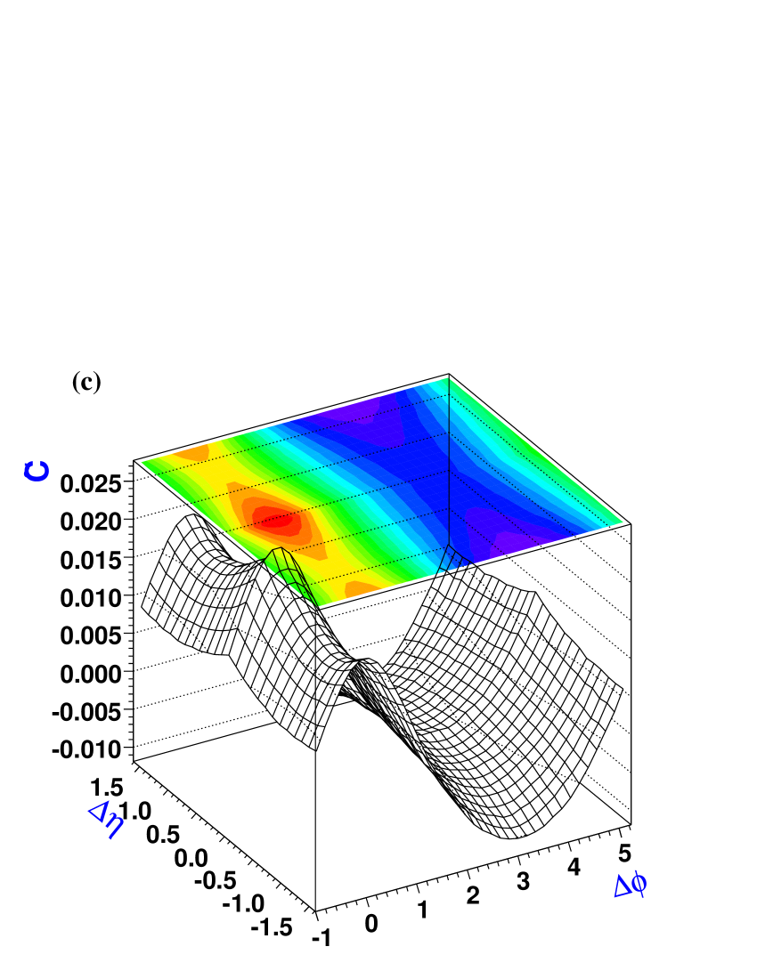
We check this result by artificially constructing events on the basis of a superposition of independent N = 15 collisions generated with PYTHIA. Figures 3(a-c) display correlation functions obtained with N = 15 independent collisions modeling collisions with 30 participants. A total of two million minimum bias events were integrated to produce these results.
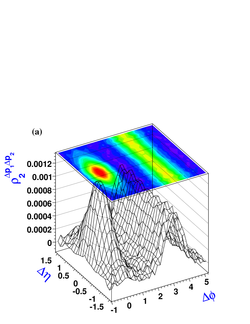
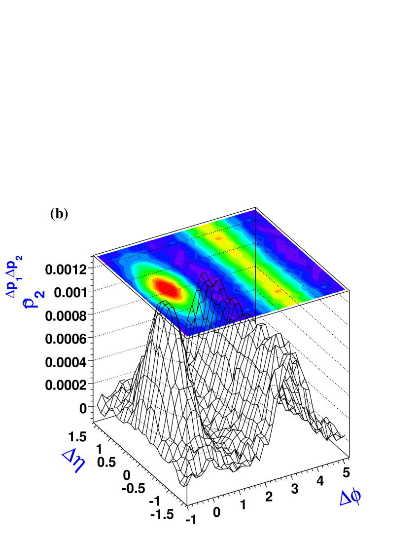
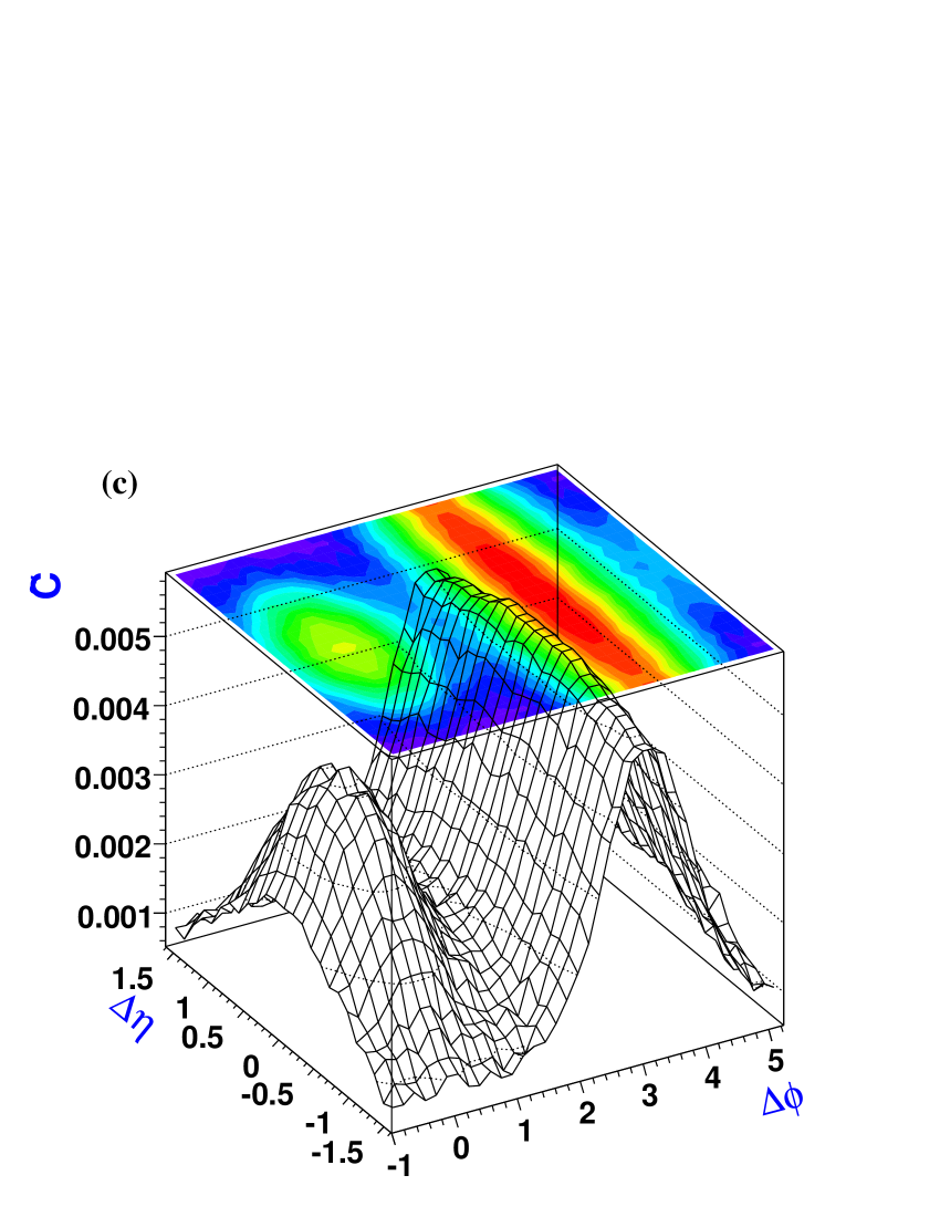
The most prominent feature observed for all the observables is the dilution of signal strength. The signal strength is diluted by a factor of 15 as compared to that found in collisions (shown in Figure 1). This effect is attributed to 15 times larger multiplicity produced for N = 15 independent collisions. The shape of inclusive and event-wise observables, with a peak-like structure on the near side and a ridge-like structure on the away side is still observed, as previously observed for Figure 1(a,b). Similarly we observe the same shape of , i.e. larger amplitude of the away side ridge vis-a-vis the near side peak.
We also present results on collisions produced by the superposition of N = 100 collisions, i.e., 200 participants. Two million minimum bias events were integrated to present the results in Figure 4(a-c). As expected, we observe the signal strength is diluted by a factor of 100.
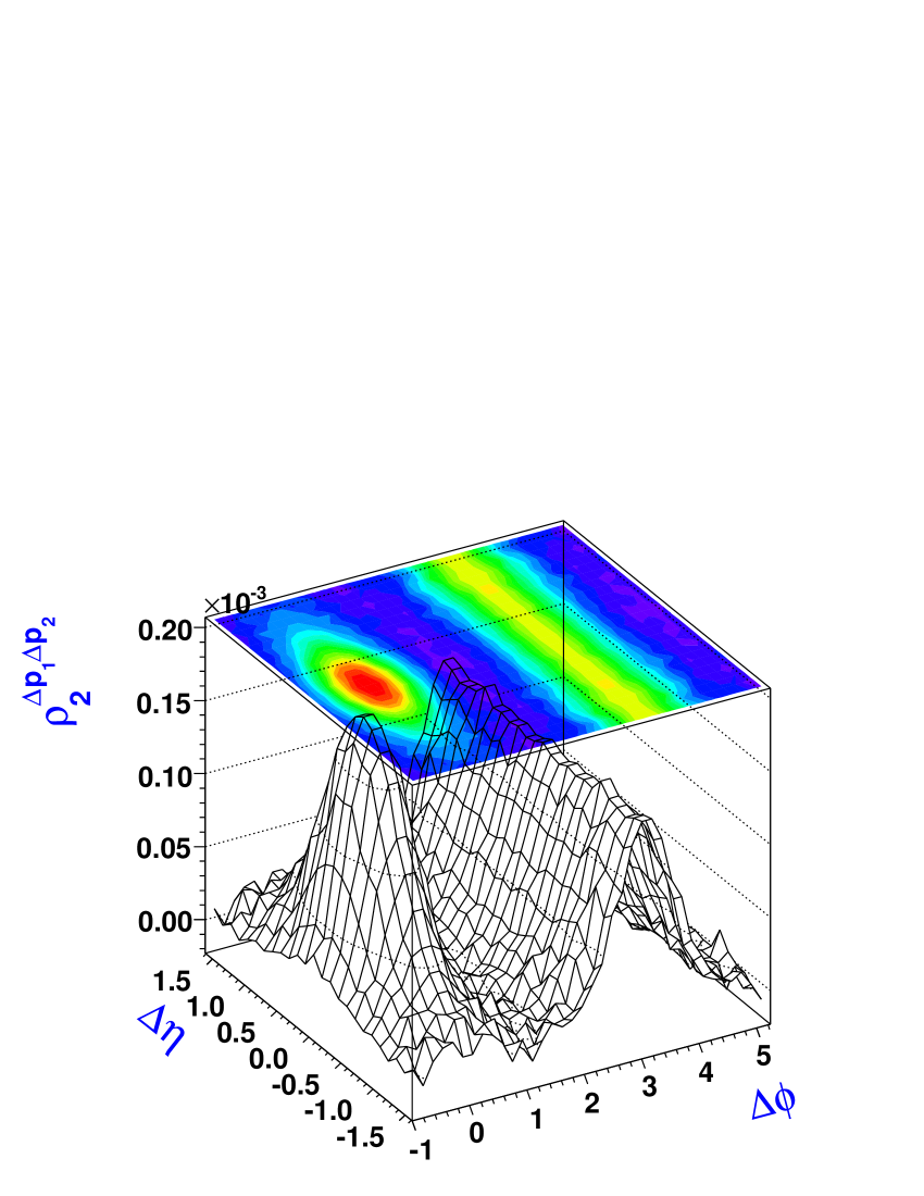
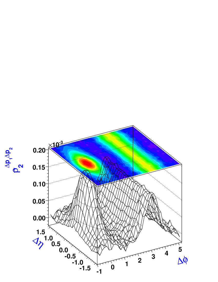
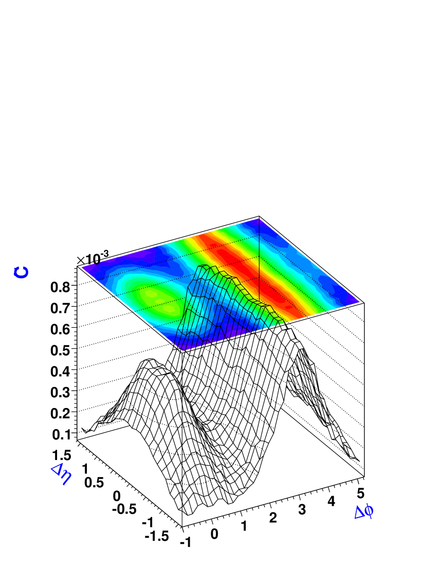
We next consider the effect of radial flow on artificially generated collisions. As for Figures 5(a-c), we produce collisions consisting of N = 15 independent interactions. Particles of a given interaction are now boosted radially in the transverse plane with . The dominant features remains the same as discussed previously for Figures 2(a-c), i.e., observation of diminished away-side ridge-like correlations and enhanced near-side correlation for all the three observables. Therefore, on the basis of simulated and collisions, we conclude that strong radial flow should shift the away side structure to the near side in collisions and thereby produce a ridge in momentum correlations.

VII Effect of Flow on transverse momentum correlations in heavy ion collisions
Flow plays an important role in heavy ion collisions. It particularly affects particle correlations in azimuth. The effect of elliptic flow on azimuthal (density) correlations is well documented WhitePapers . Here, we consider its effect on transverse momentum correlations studied as a function of relative azimuthal angles and pseudorapidity. The calculation method is similar to that used in Pruneau06 .
We model the probability density function (pdf) of particle emission as a function of pseudorapidity, azimuthal direction and transverse momentum, relative to reaction plane as follows.
| (45) |
represents the reaction plane azimuthal direction. , , and are the pseudorapidity, azimuthal emission angle and transverse momentum of the particle, respectively. is the pdf of the particle at a given pseudorapidity and transverse momentum. Explicit knowledge of this pdf is not required in the following. Assuming the reaction plane is not measured, the two-particle pdf is given by
We use Eq. 14 to calculate the inclusive correlations:
| (46) |
where and are average and weighted average of flow coefficients function as a function of pseudorapidity, respectively.
| (47) | |||||
| (48) |
and
| (49) |
We find the magnitude of the correlations associated with a flowing medium are determined by the flow coefficients weighted by the transverse momentum and the averaged transverse momentum of the system. The correlations exhibit cosine modulations in azimuth. It is observed in collisions at RHIC that flow coefficients and average transverse momentum are both functions of the pseudorapidity of the particles phobos ; brahms . We therefore expect, based on Eq. 14, the two-particle correlations associated with flow are also a function of the particles pseudorapidity difference. Azimuthal anisotropy coefficients measured at RHIC are largely dominated by elliptic flow () coefficients. Flow modulations of the inclusive correlations should then also dominated by second order harmonic coefficients.
VIII Experimental Robustness of Correlation Functions
Measurements of correlation observables in and collisions require one applies corrections for the limited acceptance and detection efficiency. In some cases, correlation functions may be formulated in such a way that detection efficiency partly cancels. This was discussed already by a number of authors for various correlation observables. See for instance Ref. NystrandTydesjo for a discussion of the robustness of factorial moments and the observable, , used in measurements of charge correlations. In this section, we investigate the extent to which the transverse momentum differential correlation functions, defined in Sect. III, are robust observables. We use simple simulations to explicitly verify the robustness of these observables in contexts where efficiencies are non-trivial functions of the particle kinematics.
Neglecting instrumental effects such as track splitting, ghost tracks etc., the single-particle and pair yields, and measured at some , , , are the products of the one- and two-particle densities by efficiencies and for measuring one- and two- particles, respectively.
| (50) | |||||
| (51) |
In the above equations, represents the measured variables , , . The ‘raw’ momentum correlation, , is thus a function of the detection efficiency. We show in the Appendix that particle losses due to limited efficiency in general lead to a modification of the fixed multiplicity momentum averages. Measurements of average momentum are consequently intrinsically non-robust. However, one also finds that if the average is independent of, or varies slowly with, the event multiplicity, one can apply Eq. 51 to evaluate the correlation functions.
| (52) |
Obviously, if the efficiency is independent of the measurement coordinates, i.e. then efficiencies cancel out in Eq. 52: the inclusive transverse momentum correlation is thus a “robust” quantity. In general, however, the efficiency is a function of the measurement coordinates. This implies corrections are required to account for detection efficiency. We note that Eq. 52 simplifies considerably if the efficiency can be factorized into separate functions of momentum and pseudorapidity. It reduces to , i.e. is robust to first order, if the efficiency is uniform across the acceptance of the measurement. Large detectors at RHIC and LHC have detection efficiencies that are reasonably uniform across their acceptance. However, various instrumental effects, such as detector boundaries or defective components, introduce small non-uniformities. We model these as follows:
| (53) | |||||
| (54) |
where and correspond to the average efficiencies for detecting one- and two-particles, respectively. The functions and represent detection non-uniformities across the detector acceptance in , and . They average to zero, by definition, over the acceptance of the apparatus. For “reasonably behaved” detectors, one typically finds
Let us assume further that . One then finds the raw two-particle momentum correlation is approximately equal to
| (55) |
where
| (56) | |||||
| (57) |
In general one has , which implies , i.e. the difference is non-vanishing. The inclusive transverse momentum correlation is indeed not perfectly robust as an observable. This implies a correction might be explicitly needed. A correction based on Eq. 54 is not practical because it requires knowledge of the two-particle density. It is thus simpler to carry an efficiency correction on a per particle pair basis, i.e. rather than counting “1” for each measured pair, increment the number of pairs according to
The above formulation of efficiency effects on the correlation neglects possible event detection biases incurred with small detection efficiency. Large particle losses may produce a significant modification of the spectrum of small multiplicity events. This is, thus, susceptible of significantly biasing the measurement of correlation of collisions.
Figure 1, discussed in Sect. V, displays PYTHIA events obtained with perfect efficiency and serves as a reference for simulations presented in Figures 7 through 8 obtained with limited detection efficiency. The effect of detection efficiency is obtained by individually and randomly rejecting particles on the basis of a given efficiency prescription,
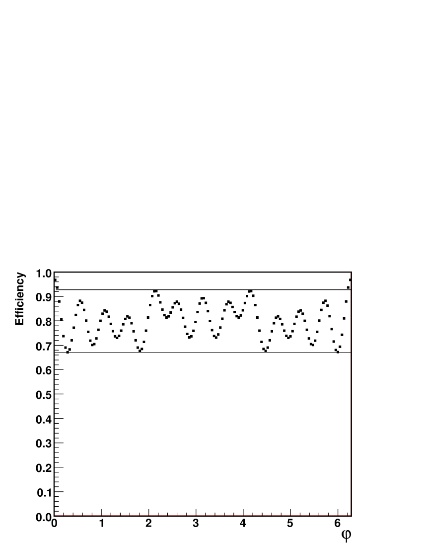
One uses a two-particle efficiency equal to the product of single particle efficiencies, as per Eq. 54. The single particle efficiency is defined on the basis of a Fourier decomposition involving twelve terms as follows:
| (58) |
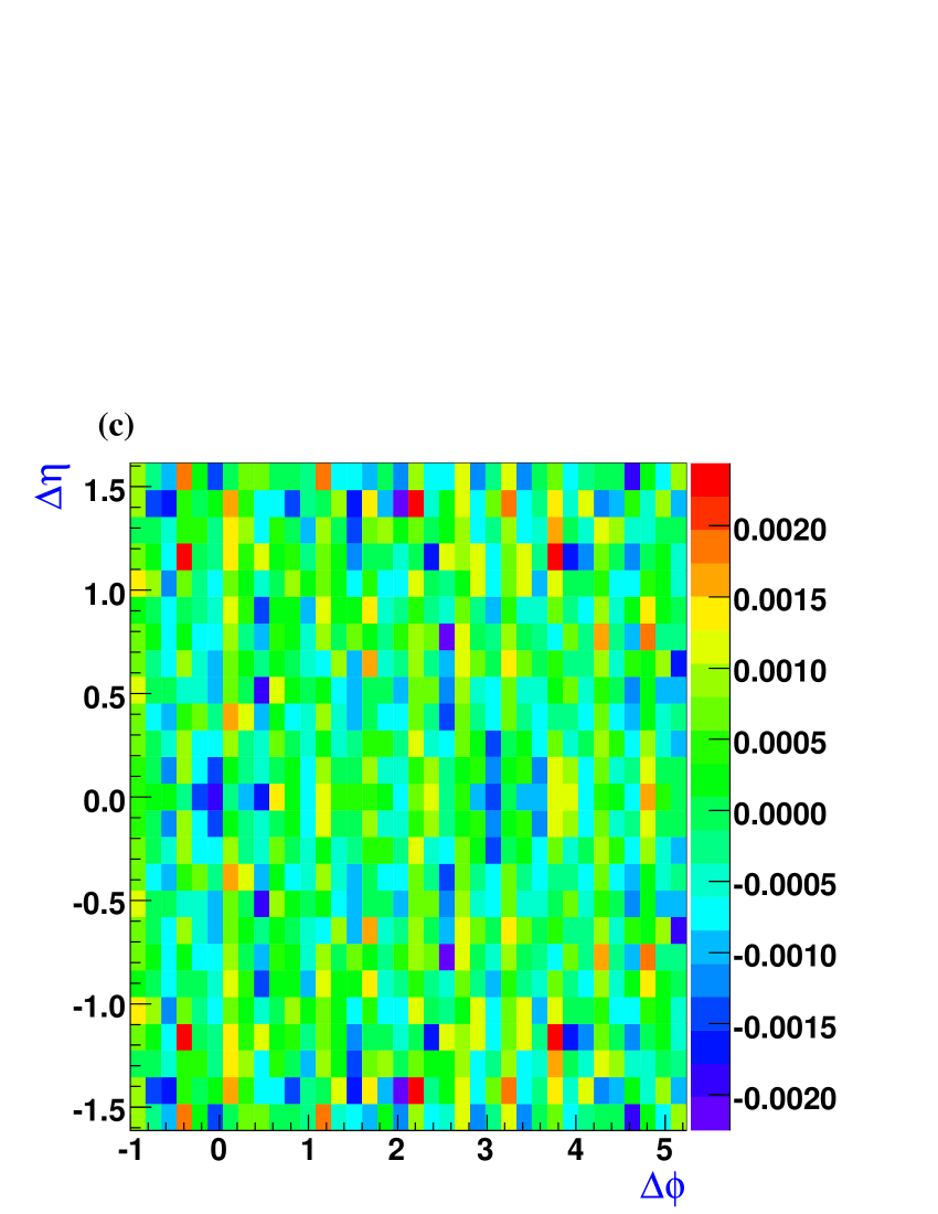
The coefficients are chosen to approximately model the azimuthal efficiency dependency of large detectors such as the STAR TPC and ALICE TPC. Spike structures are introduced in azimuth to simulate the effect of detector boundaries. Twelve sectors are used. The amplitude of the efficiency varies across the acceptance by 10%. Figure 6 shows efficiency non-uniformities introduced in azimuth. Figures 7 shows the robustness of the observables studied on the basis of Eq. 58. Our study of the impact of detection efficiency is based on single collisions generated with PYTHIA.
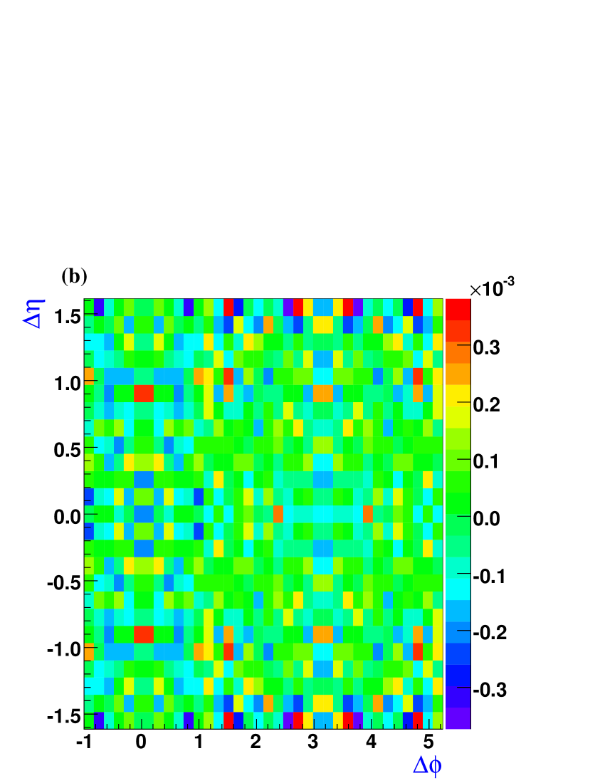
Figures 7(a-c) show correlations obtained with Eq. 58 using . For each produced particle one generates a random number, . The particle is included in the analysis provided . In Figures 7(a-c) we show the difference between the correlation functions obtained for perfect efficiency, i.e. and reduced efficiency, i.e. , for all three observables of interest. The differences in the case of inclusive and event-wise observables are of the order of 0.5% only, whereas the difference observed for is 1%. However, despite extremely small dependence on efficiency, we observe finite near-side and away-side structures in the difference. In contrast, reflects the effect of detector boundaries. There are exactly twelve structures in azimuth which correspond to detector boundaries introduced as non-uniformities in azimuth. The differences are however numerically small and amount to 1% of the signal at = = 0. We therefore conclude that all the three observables exhibit very little dependence on detection efficiency.

We next include, for illustrative purposes, a linear efficiency dependency on the particle transverse momentum.
| (59) |


Figures 8(a-c) show the difference between the correlation functions obtained for perfect efficiency, i.e. = 1 and efficiency dependent on particle transverse momentum as per Eq. 59 obtained with = 0.8. The dominant features observed in Figures 8(a-c) remain the same as those observed in Figures 7(a-c). We verified the robustness of these observables by further reducing the efficiency (Eq. 54) to 50%, i.e. = 0.5. The difference, , is of the order of 5% for inclusive and event-wise observables where as the difference for increases by 2% only. We conclude that all three observables, inclusive, event-wise and are quite robust. Their dependence on efficiency, even when it varies across the acceptance by as much as by 10%, is very small.
IX Summary and Conclusions
We introduced formal definitions and notations for inclusive, event-wise and correlation functions. We considered more specifically transverse momentum two-particle correlations expressed as functions of the particle pseudorapidity and azimuthal angle differences. We also studied a generalization of the observable proposed by Gavin Gavin , which he uses to determine the viscosity per unit of entropy of the nuclear matter produced in collisions at RHIC and the LHC.
We used the event generator PYTHIA Pythia to study and predict the shape of the correlation functions for minimum bias collisions at GeV. Simulations were carried out for particles in the ranges and GeV/c. The correlation functions exhibit a relatively narrow peak at , and a wide away-side band or ridge extending over the full range of pseudorapidity . These features are qualitatively similar to those found in particle density correlations calculated with PYTHIA Pruneau07 .
While the three observables are meant to determine the level of transverse momentum correlations between produced particles, their definitions differ significantly. One expects in the large multiplicity limit, values obtained with the three observables should be identical. However, in practice, multiplicities in a given bin of relative pseudorapidity and azimuthal angles () are rather small. This implies differences between these three observables can be substantial. We verified this expectation on the basis of collision simulations calculated with PYTHIA event generator Pythia . We observed inclusive and event-wise observables to be approximately identical. Both, however, differ significantly from . We conclude that for a precise comparative study of transverse momentum correlation functions for different colliding systems, at different energies and from different experiments, it is essential the same observable be used to characterize the correlation shape and strength.
We studied the experimental robustness of the three observables. We studied the impact of detection efficiency using PYTHIA simulated collision events with an arbitrary parameterization of the efficiency dependence on the detection angle and transverse momentum. We found that these observables are robust even when the detection efficiency reduces to 50%.
We studied the scaling of the inclusive transverse momentum correlation function with the number of participating nucleons in collisions assuming the interactions are independent and with no rescattering of the secondaries. We found that, similar to other correlation observables Pruneau03 , the correlation strength exhibits a dependence for varying collision centralities.
We additionally studied the effect of radial flow in and collisions on the magnitude and azimuthal dependence of these observables. We found that radial flow is responsible for the shift of the away side structure to the near side ridge like structure.
Acknowledgements
The authors acknowledge constructive discussions with S. Gavin and S. Voloshin. The authors also
thank L. Tarini for his careful reading of the manuscript and editorial comments.
This work was supported in part by DOE grant no. DE-FG02-92ER40713.
References
References
- (1) S. Gavin and M. A. Aziz, Phys. Rev. Lett. 97 (2006) 162302.
- (2) M. Horner et al. (STAR Collaboration), Proceedings of the Quark Matter 2006 Conference, Shanghai, China, 2006, J. of Physics G: Nuclear and Particle Physics, in press; J. Putschke, et al. (STAR Collaboration), Proceedings of Quark Matter 2006; arXiv:nucl-ex/0701074; D. Magestro, et al. (STAR Collaboration), Proceedings of Hard Probe Conference, 2004.
- (3) S. Gavin, L. McLerran and G. Moschelli, arXiv:nucl-th/0806.4718.
- (4) C. Adler et al. (STAR Collaboration), Phys. Rev. C 68 (2003) 044905.
- (5) J. Adams et al. (STAR Collaboration), Archive Number (2008).
- (6) J. Adams et al. (STAR Collaboration), Phys. Rev. C 71 064906 (2005)
- (7) C. Adler et al., (STAR Collaboration), Phys. Rev. Lett. 90 (2003) 172301.
- (8) J. Adams et al. (STAR Collaboration), J. Phys. G 34 (2007) 799.
- (9) M. Gazdzicki and S. Mrowczynski, Z. Phys. C 54 (1992) 127.
- (10) J. Adams et al. (STAR Collaboration), J. Phys. G 33 (2007) 451.
- (11) S. Gavin, M. A. Aziz, 2nd Workshop on Particle Correlation and Femtoscopy (WPCF 2006), Sao Paulo, Brazil, 9-11 Sep 2006. Published in Braz. J. Phys. 37 (2007) 1023.
- (12) S. Gavin and G. Moschelli, Proceedings of Quark Matter 2008, Jaipur, India, 2008; arXiv:0806.4366.
- (13) T. Sjeostrand, Comp. Phys. Commun., 82 (1994) 74.
- (14) S. A. Voloshin, Phys. Lett. B 632 (2006) 490.
- (15) S. A. Voloshin, J. Phys. Conf. Ser. 50 (2006) 111.
- (16) S. A. Voloshin, V. Koch and H. Ritter, Phys. Rev. D 60 (1999) 024901.
- (17) L. Stodolsky, Phys. Rev. Lett. 75 (1995) 1044.
- (18) R. Korus and S. Mrowczynski, Phys. Rev. C 64 (2001) 054906.
- (19) M. Stephanov, arXiv:hep-ph/0110077.
- (20) K. Adcox et al. (PHENIX Collaboration), arXiv:nucl-ex/0203015.
- (21) S. A. Voloshin, Proceedings of International Nuclear Physics Conference, 610 (2002) 591; Nucl. Phys. A 749 (2005) 287.
- (22) H. Sako and H. Appelshauser, (CERES Collaboration), J. Phys. G 30 (2004) 1371.
- (23) H. Appelshauser et al. (NA49 Collaboration), Phys. Lett. B 459 (1999) 679.
- (24) J. Adams et al. (STAR Collaboration), Phys. Rev. C 72 (2005) 044902.
- (25) C. Pruneau, S. Gavin and S. A. Voloshin, Nucl. Phys. A 802 (2008) 107.
- (26) I. Arsene et al. (BRAHMS Collaboration), Nucl. Phys. A 757 (2005) 1; K. Adcox et al. (PHENIX Collaboration), ibid. 184; B. B. Back et al. (PHOBOS Collaboration), ibid. 28; J. Adams et al. (STAR Collaboration), ibid. 102. K. H. Ackermann, et al., (STAR Collaboration), Phys. Rev. Lett. 86 (2001) 402.
- (27) C. Pruneau, Phys. Rev. C 74 (2006) 064910.
- (28) B. B. Back et al. (PHOBOS Collaboration), Nucl. Phys. A 715 (2003) 65.
- (29) I. G. Bearden et al. (BRAHMS Collaboration), Phys. Rev. Lett. 94 (2005) 162301.
- (30) J. Nystrand, E. Stenlund and H. Tydesjo, Phys. Rev. C 68 (2003) 034902.
X Appendix
Experimentally, one measures at a given , , and a number of particles . This number is divided by the bin size to obtain the uncorrected density . In general, the detection efficiency is a function of all three coordinates herein noted , , . The actual density, , is obtained as follows:
| (60) |
The efficiency changes as detector conditions evolve over time. It may also be a complicated function of the measured event structure. It is the case for instance with a TPC in heavy ion collisions measurements. One observes experimentally that the detection efficiency depends on the detector occupancy, or particle track multiplicity in the detector. At low multiplicity, tracks are on average well separated and hence easy to identify and reconstruct. However, for large multiplicity, the distance between tracks is reduced such that they may cross and partially overlap. The efficiency is consequently a function of the event multiplicity as well as the beam luminosity. The dependence on luminosity may be corrected for by estimating , , based on embedding techniques. We parameterize this dependence on global event factors with an index . For convenience, one writes the detection efficiency at given multiplicity as follows:
| (61) |
where represents the averaged efficiency, and B is a normalized response function.
| (62) |
The number of particles detected at given and is written as
| (63) |
The measured average particle is then
| (64) |
and is clearly not a robust quantity. However, in cases where the average is measured over a small range of multiplicity, one has
| (65) |
while this expression indicates the measured average still depends on the detector response, it is easy to verify that in cases where the dependence is ÔmildÕ, the above expression is a reasonable approximation of the actual average momentum. Consider for instance a case where the density has an exponential dependence on the momentum where is a slope parameter describing the particle distribution. We evaluate the impact of the detector response using a linear approximation . Assume T has a value of 0.6. The average changes by 1% relative to the actual average when the value of the response parameter is chosen to be 0.05. Smaller values of lead to smaller deviations. One thus finds that unless is exceedingly large, the detector response has a rather limited impact, a few percent only, on the measured average momentum. It is, nonetheless, a function of the detection coordinates and : deviations of measured may depend on and . The above argument is straightforwardly repeated for measurements of correlations . Given this quantity depends essentially on the square of the detector response, one expects the impact of a dependence should be rather small - although potentially a function of the particle coordinates , , and .